State-Dependent Stock Liquidity Premium: The Case of the Warsaw Stock Exchange


Department of Corporate Finance, Institute of Accounting and Finance Management, Poznań University of Economics and Business, 61-819 Poznań, Poland
Int. J. Financial Stud. 2020, 8(1), 13; https://0-doi-org.brum.beds.ac.uk/10.3390/ijfs8010013
Submission received: 28 December 2019
/
Revised: 25 February 2020
/
Accepted: 2 March 2020
/
Published: 6 March 2020
Abstract
:The effect of stock liquidity on stock returns is well documented in the developed capital markets, while similar studies on emerging markets are still scarce and their results ambiguous. This paper aims to analyze the state-dependent variance of liquidity premium in the Polish stock market. The Polish capital market may serve as a benchmark for other emerging markets in the region of Central and Eastern Europe, hence the results of this research should be of great interest for investors and policy makers in Poland and other post-communist European countries. In the empirical, study a unique empirical methodology has been applied, which guarantees the uniqueness of the results obtained. The results obtained suggest that on the Polish stock market exists stock liquidity premium, which is statistically significant, but constitutes only a small fraction of returns. It also does not increase during periods of bearish market, what results from the lengthening of average holding period when market liquidity decreases.
Keywords:
liquidity premium; Warsaw Stock Exchange; pricing of liquidity; liquidity costs; amortized liquidity costsJEL Classification:
G11; G121. Introduction
Liquidity premium is related to the existence of the relationship between security liquidity and its expected rate of return. The fact that less liquid shares yield higher returns than more liquid ones, associated with the positive liquidity premium, is well documented in the US and other developed stock markets. However, not all studies confirm the existence of this relationship, in particular on relatively less-developed capital markets. One should also pay attention to the scarcity of such studies on emerging capital markets.
The main objective of this paper is to analyze the state-dependent variance of liquidity premium in one of the leading European emerging markets, namely the Polish one. The contribution of the paper is at least threefold. First, the paper contributes to the literature, as this is one of the first papers considering conditional, i.e., time-varying, liquidity premium. Most of the empirical research is focused on indicating the unconditional, i.e., constant over time, liquidity premium. However, as pointed out by some authors (e.g., Jensen and Moorman 2010; Amihud 2014; Hagströmer et al. 2013; Ben-Rephael et al. 2015) the amount of liquidity premium may be time-varying. There is still a lack of a comprehensive answer to the question about the factors determining the amount of such a premium. This problem is mostly highlighted by Holden et al. (2014, p. 349), who point out that time-variance of liquidity premium requires further analyses. In particular, most important is the indication of factors determining its amount, for example, whether it increases during crises or if it varies across the business cycle.
The second important contribution emerges from the empirical approach in investigating liquidity premium. To the best of the author’s knowledge, this is the first study in which the relationship between liquidity and returns was analyzed on a single stock level (rather than on a portfolio level) with the use of panel data. The use of the data on a single stock is justified by the fact that liquidity costs are undiversifiable (Amihud and Mendelson 1986) and the use of portfolios instead of single stocks may lead to the loss of some important information. Moreover, in regressions carried out, liquidity measure is amortized similar to Chalmers and Kadlec (1998) and unexpected stock liquidity is included. Some of the previous studies take into account the unexpected liquidity, but at the market, not a single stock, level (Amihud 2002; Goyenko 2006).
Finally, this study contributes to the literature as it utilizes data on stocks listed on the Polish stock exchange, which is still considered an emerging market. Warsaw Stock Exchange (WSE) provides an interesting setting for studying liquidity premium as it differs significantly from the US stock markets. The market is dominated by long-term investors, such as the state treasury, open pension funds, institutions (including SOEs), and families. WSE is also densely populated by small and medium entities, and trading is concentrated within the small number of blue chips. The smallest 290 companies (60% of total listed stocks) account for only 2.19% of total capitalization, compared to 13% in the US market. The most thinly traded 290 companies (60% of all listed stocks) accounts for only 0.55% of total turnover, and 80% of the turnover is concentrated in the 11 most heavily traded stocks (2.28% of all companies).
The Warsaw Stock Exchange is an order-driven market, which means that its trading mechanism differs from the quote-driven mechanism displayed in the US stock markets. Liquidity concerns may be of less importance in order-driven markets than in the quote-driven ones, as the order imbalance spreads between a large number of liquidity providers, rather than concentrating on one market maker. Hence, the study contributes the literature on liquidity premium in non-US order-driven markets. However, the Polish stock market is far less developed and less liquid than most developed markets around the world. Thus, stock liquidity should play a more important role in asset pricing than in the US (see e.g., Bekaert et al. 2007).
At the beginning of 21st century, WSE was the largest and fastest-growing market in Central and Eastern Europe, making it an interesting field of study. The WSE has a lot of companies from different European countries listed (e.g., Czech, Slovakia, Slovenia, Ukraine, Hungary, Lithuania, Austria, Germany, Netherlands, Spain, Italy, and United Kingdom), it can also be viewed as a very important stock market in Europe and serves as a benchmark for other emerging stock markets in post-communist European countries.
The above-mentioned differences between the Polish and US stock markets may cause the results of the studies carried out on the Polish stock market to differ from the respective results of the studies carried out on the US stock market. On the one hand, as the WSE is a less developed and less liquid market, stock liquidity should influence the stock returns more severely than on the US one. On the other hand, the fact that the WSE is an order-driven market should attenuate this relationship. Equally important, studies carried out so far do not allow to indicate clearly if there exists a stock liquidity premium in the Polish capital market. Previous research is scarce and their results varied. This is the first such extensive study on the liquidity premium in the Polish stock market. The study covers all common stocks listed on the Warsaw Stock Exchange in the period from 2001 to 2016.
The obtained results indicate that there exists a liquidity premium in the Warsaw Stock Exchange. The study allowed also to state that liquidity premium is in part captured by the return on the market portfolio and by the premiums related to a firm’s size and value. Although statistically significant, stock liquidity premium is only slightly economically relevant in the Polish capital market. The results indicate that in the periods of bear market, when the overall level of liquidity decreases, investors lengthen the investment horizon, thus reducing the frequency of trading and, equivalently, the frequency of incurring the liquidity costs. This leads to the lack of statistical significance of the difference in liquidity premium during the bull and bear market phases.
The rest of the paper is organized as follows. The following part is devoted to methodological issues of the study, it describes the empirical framework utilized, methods applied, variables, and the sources of data. Section 3 provides the empirical results and the series of robustness tests is presented in Section 4. The final section concludes.
2. Literature Overview
Stock liquidity is a broad and elusive concept. The level of liquidity can be defined as the extent to which an investor is able to trade (buy or sell) large quantities of a security at any time, at no cost, and without causing an unfavorable movement in the security’s price. Defined as such, liquidity is hard to measure as it encompasses several dimensions, i.e., time (immediacy), quantity (depth), cost (tightness), and price impact (resiliency).
The first paper, in which the relationship between stock liquidity and stock returns was empirically analyzed is the article of Amihud and Mendelson (1986). The results of their study were then verified by Eleswarapu and Reinganum (1993), who claimed that the observed relationship is constrained only to the month of January. As one of the most important studies in the field of liquidity premium, one should mention the papers of Brennan and Subrahmanyam (1996), Datar et al. (1998), and Amihud (2002). Another milestone in studies on the relationship between liquidity and stock returns, by considering the time-variance of the level of liquidity, was put by Pástor and Stambaugh (2003). Pástor and Stambaugh’s (2003) studies have been developed in the paper of Acharya and Pedersen (2005). An important part of the global trend of research in the field of dependence between liquidity and returns is also the work of Liu (2006) who constructed the Liquidity-Augmented Capital Asset Pricing Model. In addition, Lee (2011) and Amihud et al. (2015) tested the existence of liquidity premium in the international setting.
The study by Amihud and Mendelson (1986) remains one of the most important pieces of research on stock liquidity premium. Since they published their paper, one may observe a growing interest in this subject, resulting in a constantly increasing number of papers, both theoretical and empirical, regarding liquidity premium. Repeatedly, the conclusions of theoretical research stand in opposition to the results of empirical research. Empirical studies indicate liquidity premium is much higher than that which should be observed in line with the theoretical analyses. However, most of the research carried out on the US and other developed stock markets indicate the existence of a significant positive liquidity premium.
Similar studies carried out on less-developed markets do not provide unambiguous results. For instance, Bekaert et al. (2007) studied 19 emerging markets and found significant liquidity premium across these markets. Similarly, Amihud et al. (2015) analyzed 19 emerging and 26 developed markets and found liquidity premium higher in emerging than in developed markets. On the contrary, Stereńczak et al. (2020) studied liquidity premium in 22 frontier markets and found it insignificantly negative. The same was found by Batten and Vo (2015), who analyzed the Vietnamese stock market, included in the research sample by Stereńczak et al. (2020). The rationale of Batten and Vo (2015) and Stereńczak et al. (2020) for the existence of insignificant negative liquidity premium is that frontier markets provide unique diversification benefits that offset stock illiquidity.
Similarly, previous research on the Polish stock market (Warsaw Stock Exchange, WSE) is scarce and gave ambiguous results. One may conclude that there is still no comprehensive answer about the existence of liquidity premium in the WSE. Gajdka et al. (2010), Gniadkowska (2012), Gniadkowska-Szymańska (2018), Garsztka and Rutkowska-Ziarko (2012), and Stereńczak (2017) found significantly positive stock liquidity premium in the Polish market, while Włosik (2017), Nowak (2017), Lischewski and Voronkova (2012), Olbryś (2014), and Piotrowski (2015) have claimed no significant relationship between liquidity and stock returns in the Polish stock market.
Most of the extant empirical research on liquidity premium is focused on indicating the unconditional, i.e., constant over time, liquidity premium. Only recently, Jang et al. (2015) analyzed state-dependent liquidity premium on the Korean stock market. They found that liquidity premium differs significantly in different market states. In particular, they found that realized liquidity premium is significantly higher in the expansive state, rather than in the recession state. Market states were distinguished based on two variables: the business cycle indicator for recessions and expansions provided by Statistics Korea, and unexpected innovation in monetary base. Their research, thus relied on the effect of funding liquidity on market liquidity, theoretically developed by Brunnermeier and Pedersen (2009). Hence, one may say that the distinction of market states has been made only indirectly.
Jang et al. (2017) analyzed state-dependent variations in the expected liquidity premium in the US stock markets (NYSE/AMEX/NASDAQ). Using bivariate Markov-switching models, they proved that various factors (default spread, term spread, growth in money stock, and Treasury bill rate) predict future stock returns for portfolio of low-liquid stocks differently than for portfolio of high-liquid stocks. As a result, expected liquidity premium displays strong state-dependent, countercyclical variations.
Grillini et al. (2019) developed and estimated regime-switching Liquidity-Adjusted Capital Assets Pricing Model (L-CAPM) by Acharya and Pedersen (2005) to indicate the time-variant pricing of various liquidity risks within the seven Eurozone countries (all developed ones). Chulia et al. (2019) used the conditional quantile regression approach to present time-variations in liquidity pricing according to the state of the market. These two papers display different approach to pricing of stock liquidity, i.e., they treat liquidity as a risk factor, not the stock characteristic. To briefly summarize, studies on conditional (time-variant) liquidity premium is scarce and focused on US and other developed markets. Only the study of Jang et al. (2015) is devoted to the Korean market; however, it presents an indirect approach to the distinction of market states.
3. Methodology and Data
3.1. Empirical Framework and Hypotheses Development
The costs related to imperfect liquidity of a stock (liquidity costs) are incurred by investors twice—at the beginning and at the end of the investment. The existence of liquidity costs lowers the returns obtained from the investment, therefore a rational investor will make such a valuation of the shares at the time of purchase, to ensure that he receives the required rate of return. While making the valuation, thus specifying the maximum price that he is willing to pay for a given stock, an investor should take into account liquidity costs incurred at the time of purchase and sale, as well as the price at which they will be able to sell the stock. The latter one in turn depends on the future liquidity costs and return required by investor who will buy this share in the future. Thus, a series of transactions is created, during which liquidity costs are incurred. At the end of this series, the last stockholder will receive a certain liquidation value of the share.
Let us assume that investors’ expectations as to the stock liquidation value and investors’ required returns are homogenous. One may indicate that current stock price is a function of its liquidation value, expected return, and the present value of liquidity costs, incurred each time the stock changes the owner. A similar conclusion, limited only to the one of the components of liquidity costs, namely bid-ask spread, was already presented by Amihud and Mendelson (1986, p. 228).
Therefore, it is reasonable to believe that at the time of purchase, an investor will take into account present and future level of stock liquidity (Eleswarapu 1997, p. 2122). However, what is evidenced by many empirical studies is the level of liquidity fluctuates over time that results in the uncertainty as to the liquidity costs needed to incur at the moment of the sale of the stock (Amihud et al. 2005, p. 286). It also increases the uncertainty as to the price for which an investor will be able to sell the stock.
In summary, when purchasing the shares, an investor will make such a valuation, which will ensure that he will obtain the required return, taking into account liquidity costs incurred presently and in the future. Less liquid shares, and therefore charged with higher liquidity costs, should thus yield higher returns than less-liquid shares. According to previous research (among others Amihud and Mendelson (1986), Chalmers and Kadlec (1998), Næs and Ødegaard (2009), Anginer (2010), Florackis et al. (2011)) the effect of liquidity on stock returns depends not only on the amount of liquidity costs, but also on the frequency of transactions, and thus the frequency of incurring these costs. This is directly related to the length of the holding period (investment horizon). Liquidity costs are incurred only when buying and selling, which means that the longer the holding period, more periods can be divided into liquidity costs. Therefore, the required compensation in rates of return (liquidity premium) per one period should decrease with an increase in the investment horizon.
Liquidity premium may be time-varying, which has been empirically documented in several studies. Most of the factors that have been identified as affecting the amount of the liquidity premium in previous research can be, directly or indirectly, related to the economic situation, or more accurately—to the bull and bear market phases. Such factors include, but are not limited to: the return on market portfolio, market volatility (risk), level of market liquidity, volatility of liquidity, and the level of founding liquidity.
Taking into account the above considerations, the following research hypotheses have been adopted:
Hypotheses 1 (H1).
More liquid shares yield lower returns than less liquid shares.
Hypotheses 2 (H2).
Stock Liquidity premium is higher during the bear market than during the bull market.
The setting is as follows. A marginal investor makes an investment decision at the end of the month t − 1. Based on the level of liquidity in month t − 1, and thus the level of liquidity costs at the time of purchasing shares, he forecasts the level of liquidity in the future, at the moment of sale. Then, he makes a decision regarding the investment horizon, and taking into account the return he requires and the incurred liquidity costs amortized over the investment horizon, makes a valuation of the share, specifying the maximum price he is willing to pay for that stock. This valuation is observable directly at the end of the month t − 1. The expected rate of return is observable indirectly, by analyzing the stock price at the end of the month t. Also, the decision of the marginal investor about the investment horizon is directly unobservable. Indirectly, one can conclude its choice by observing the turnover ratio in month t—the longer the investment horizon, the lower the turnover ratio in that month. The setting has been presented in a simplified form in Scheme 1.
As stock liquidity is time-varying (Amihud et al. 2005), predictions by an investor of future level of stock liquidity is charged with an estimation error. Expected rate of return is a function of stock characteristics, i.e., liquidity costs at the beginning (month t − 1) and the end of the investment. Expected return is observable only indirectly through the realized return in the month following the beginning of the investment (month t). Realized return may be a biased estimate of expected return as liquidity level in month t may differ from the predicted one. This causes the need to include the unexpected level of liquidity in an empirical model to analyze the effect of stock liquidity on expected returns. If unexpected liquidity is not be taken into account in a model, estimated liquidity premium could be biased downwards. This is in line with Amihud (2002), who proved that ex ante returns are an increasing function of expected illiquidity, and unexpected illiquidity has a negative effect on contemporaneous stock returns.
Taking into account this setting, the relationship between stock liquidity and returns may be verified by the estimation of the following model:
where Liqit denotes the value of liquidity measure for i-th stock in month t, while superscripts E and U are related to expected and unexpected level of liquidity respectively, and Xit is a vector of control variables.
Unexpected level of liquidity is most often determined based on the autoregression model, which means that and are colinear, as:
The first part of the right side of the formula (2) can be written as , while the residual is the unexpected liquidity (). Substituting in Equation (1) with the first part of the right side of Equation (2) gives the following:
Thus, the model described by the Equation (1) can be rewritten as follows:
where and . Estimated reflects liquidity premium per unit of amortized liquidity costs, and estimated reflects the effect of unexpected liquidity on contemporaneous stock returns.
Following the abovementioned setting, the second hypothesis can be verified by estimating the following model with the use of interactive variables:
where Ht and Bt are dummy variables that equal to 1 if month t is considered to be the bull and bear market period respectively, and 0 otherwise. Thus, estimated and reflect per unit liquidity premium during bull and bear market respectively, and estimated and reflect the effect of unexpected liquidity on contemporaneous stock returns during bull and bear market respectively. However, the use of interactive variables requires the identification of bull and bear market periods on the Warsaw Stock Exchange during the analyzed period. For this purpose, Markov-switching models will be utilized.
3.2. Variables
Model (4) will be estimated using differently defined stock returns (r*). In particular, the following definitions of rates of return will be applied:
- raw returns:
- excess returns:
- CAPM-adjusted returns:
- FF3-adjusted returns:
- Carhart-adjusted returns:
As the risk-free return (rft) has been utilised the one-month Warsaw Inter-Bank Offered Rate (WIBOR 1M). Values of the Warsaw Stock Exchange Index (WIG) were used as a proxy for the value of market portfolio, so the return on market portfolio (rMt) is calculated based on the relative change in the value of WIG. Size and value factors (SMB and HML) are constructed from raw data based on the original methodology of Fama and French (1992, 1993), and momentum factor (UMD) is constructed from raw data with the use of the original methodology of Carhart (1997). Parameters of pricing models for month t are estimated with the use of data from the previous 36 months (from t − 36 to t − 1), therefore β coefficients can take different values in consecutive months.
The use of several differently defined, instead of one, rates of returns is justified for at least two reasons. As pointed out by Chordia and Subrahmanyam (2004), the use of excess return reduces the cross-sectional correlation of the residuals. Furthermore, different method of estimating rates of return leads to different conclusions regarding the existence of liquidity premium. For instance, Chen and Kan (1995) did not find the relationship between liquidity and CAPM-adjusted returns, while Aït-Sahalia and Yu (2009) and Florackis et al. (2011) did. In fact, the latter ones indicated that the relationship between liquidity and stock returns vanishes when FF3-adjusted or Carhart-adjusted returns are considered. This in turn is in opposition to the results of Avramov and Chordia (2006) and Goyenko (2006), who showed that liquidity premium exists even if returns are FF3-adjusted and Carhart-adjusted. More interestingly, Machado and Medeiros (2013) pointed out that liquidity premium is even stronger when returns are risk-adjusted. Thus, the use of five differently defined stock returns will make the results more robust.
For the purpose of measuring liquidity, the Fong et al. (2017) measure has been applied. This measure has been indicated by Stereńczak (2019a) as the best proxy for liquidity for the purposes of asset pricing studies on the Polish stock market. This measure is highly correlated with various versions of the bid-ask and effective spreads, and estimates them with low error. Thus, this metric performs very well in estimating liquidity costs in the WSE. It is calculated as follows (Fong et al. 2017):
where Zerom denotes the proportion of zero-return days in month m, σm is the volatility of daily returns in month m and ϕ is the cumulative standardized normal distribution.
To minimize the influence of outliers on the analyzed relationship, values of liquidity measure have been cross-sectionally winsorized at the 2.5 and 97.5 percentile of distribution. Next, computed and winsorized values of FHT measure have been “amortized” to reflect the amount of liquidity costs per month. Amortization is done by dividing the value of liquidity measure by the average investment holding period in months. An inverse of turnover ratio has been used as a proxy for investment horizon.
The unexpected level of liquidity is calculated as a residual from the AR(1) model. A similar approach was applied by Amihud (2002), Goyenko (2006), Lee (2011), and Belkhir et al. (2018), but they estimated unexpected liquidity for the entire market, and not for the single stock.
Models (4) and (5), estimated in order to verify assumed hypotheses also include control variables, which is necessary to take into account the effect of different stock characteristics on the rates of return. The set of control variables includes:
- natural logarithm of the market value of equity (ln(MV))—to take into account the size effect (Fama and French 1992, 1993),
- book-to-market value of equity (BV/MV)—to take into account the effect of company’s value (Fama and French 1992, 1993),
- dividend yield (DY)—to control for the effect of liquidity on dividend policy (Banerjee et al. 2007; Griffin 2010; Igan et al. 2011; Stereńczak 2018b),
- cumulative return from the last twelve months (rt-12-t-1)—reflecting the momentum effect (Jegadeesh and Titman 1993),
- standard deviation of monthly returns from the last 36 months (σ) or the standard error of residuals from estimated pricing model (σε)—reflecting stock risk and stock residual risk respectively.
3.3. Data
The study covers all common stocks listed on the Warsaw Stock Exchange in the period from 2001 to 2016, which means that it is carried out on the unbalanced panel of companies. Exclusion of the earlier period is dictated by the fact that in November 2000, the WARSET trading system was introduced. Prior to the introduction of WARSET, WSE was poorly developed and its liquidity was very low, which could negatively influence the quality of obtained results.
Data needed to compute both dependent and explanatory variables, in particular stock rates of return and liquidity measures, come from various sources. Data on daily quotations have been downloaded from the InfoStrefa service and corrected for corporate actions. Data on companies’ capitalizations, book values of its equity, the number of shares outstanding, and dividend yields were obtained from the Official Quotations of Warsaw Stock Exchange (Ceduła GPW).
4. Empirical Results
4.1. Liquidity Premium in the Warsaw Stock Exchange
As the data used is a panel, in order to indicate the most appropriate method of estimation of model parameters, a series of panel diagnostic tests were carried out. The choice of the method of estimation was made based on the results of the following tests: Wald’s test on the differentiation of the intercept between panel units, Breush–Pagano test on the differentiation of the variance of residuals between panel units and Hausman test on the consistency of the GLS estimator with random effects. Conducted diagnostic tests indicated that the most appropriate method of estimation is the use of the fixed effects (FE) estimator. Binary variables reflecting fixed effects for the time units were also included in the model. The Wald test confirmed joint significance of time unit dummy variables in all estimated models. The results of the estimation are presented in Table 1. The approach developed by Arellano was applied to estimate standard errors robust to heteroskedasticity and autocorrelation (HAC).
Signs of the estimates of the parameters for control variables were consistent with the expectations. Larger companies yield lower returns than smaller ones, which is in line with the indication of Fama and French’s (1992, 1993) three-factor model. Similarly, positive estimates of the parameters for book-to-market ratio are in accordance with Fama–French three-factor model. Estimates of the parameters for the cumulative rate of return from previous twelve months were positive and statistically significant, which indicates the occurrence of the momentum effect (Jegadeesh and Titman 1993). Dividend-paying companies yield higher returns, as evidenced by the positive estimates of the parameters for dividend yield; however it should be pointed out that these estimates are statistically insignificantly different from zero.
The only estimates inconsistent with the expectations are the estimates of the parameters for variables reflecting risk and residual risk of the stock. These estimates are negative and statistically significant at the level 0.01. This indicates that investors in Poland require lower returns from more risky shares, which may be concluded that they are risk-lovers rather than risk-averts. Nevertheless, this is not the only empirical study where the estimate of the parameter for risk is negative. For example, Chalmers and Kadlec (1998) reported a parameter for return volatility equal to −1.35 with p-value 0.02. However, the negative signs of the estimates of the parameters for stock risk may be the result of some biases in the model specification. At first, one should point out that liquidity and volatility often are not independent variables (Będowska-Sójka and Kliber 2019). Second, in the research sample correlation between risk and size of the company exceeds 0.4., and last, but not least, for some panel units, time-series of volatility may be non-stationary. To omit these problems, the following modifications were applied to the specification of the models: (1) risk variable was orthogonalized versus liquidity variable, (2) risk variable was orthogonalized versus size variable, (3) risk variable was omitted, and (4) study period was divided into subperiods. Estimates of the modified M1 model are provided in Table 2. Change in the specification of the model did not change the results—in each model, the estimate of the parameter for risk is negative and statistically significant, and the signs of remaining estimates remain the same.
Regardless of the definition of stock return as a dependent variable in a model, an estimate of the parameter for the amortized liquidity measure is positive and statistically significant at the 0.01 level. This means that there exists statistically significant liquidity premium on the Warsaw Stock Exchange, which gives support for hypothesis H1. The estimate ranges from 2.394 to 2.667 with mean value 2.5, which means that investors demand to be compensated more than twice for the incurred liquidity costs, amortized over the investment horizon. As the parameter for amortized liquidity measure is related to liquidity costs incurred both at the purchase and at the sale, it is justified to expect the value of this parameter close to 2.
Chalmers and Kadlec (1998) reported the estimate of the parameter for amortized spread ranging from 4.12 to 7.89 with mean value equal to 5.29. This means that liquidity premium in the WSE is lower than respective premium found by Chalmers and Kadlec (1998) for AMEX and NYSE. This seems surprising as WSE is far less developed than US stock markets and thus should offer much higher liquidity premium. This evidence contradicts the results of previous research by Bekaert et al. (2007) and Amihud et al. (2015) and may indicate that in order-driven markets (like WSE) liquidity concerns are of less importance than in quote-driven markets (like US stock markets).
One should pay attention that the estimate of the parameter for amortized liquidity measure decreases with an increase in the number of factors explaining “normal” rates of return, i.e., in model M3 this estimate is lower than in M1, in model M4 it is lower than in M3, and in model M5 it is lower than in M4. This suggests that liquidity premium is, at least partially, captured by the market risk premium and size, value, and momentum factors. The above is in line with Aït-Sahalia and Yu (2009) and Florackis et al. (2011), who found that the use of FF3-adjusted or Carhart-adjusted stock returns causes liquidity premium being insignificant, while the use of CAPM-adjusted stock returns causes liquidity premium being significant. This also contradicts the evidence of Machado and Medeiros (2013) who claimed that stronger liquidity premium is observed after adjusting stock returns for risk.
As mentioned, the mean value of the estimate of the parameter for amortized liquidity costs equals 2.5, which is a quite reasonable value. The estimate of this parameter reflects the amount of liquidity premium required by investors for the unit of amortized liquidity costs, not the total liquidity premium. Based on this value, one cannot infer what fraction of the rate of return constitutes the observed liquidity premium. In order to determine this, the average total liquidity premium was calculated.
The average total liquidity premium was computed as the estimate of the parameter for amortized liquidity measure multiplied by the median value of amortized FHT measure. The mean value of amortized FHT measure was not used due to the high asymmetry of distribution, resulting in the lack of robustness of the mean value for the outliers. The average total liquidity premium on the Warsaw Stock Exchange is equal to 0.019 p.p. monthly, which is 4.65% of the average and 2.93% of the median rate of return on the WSE in the analyzed period. Estimated total liquidity premium is significantly lower than that reported, e.g., by Amihud et al. (2015) for emerging markets. Mean (median) liquidity premium reported in their study ranges from 0.741 to 1.161 p.p. (0.786 to 1.062 p.p.) monthly.
It can therefore be concluded that the average liquidity premium on the Warsaw Stock Exchange in the analyzed period is not highly relevant as it constitutes only a small fraction of returns. It is quite surprising that, despite the existence of significant liquidity costs, the liquidity premium seems to be only slightly relevant on the Polish stock market. It is difficult to clearly indicate if this is a positive or negative phenomenon. On the one hand, relatively small economic relevance of liquidity premium, with a relatively low level of liquidity, may indicate that the low liquidity of the WSE was not an obstacle of its development. However, on the other hand, such a situation may indicate two alternative facts: either investors in Poland are not aware of the role of liquidity in the investment process on the securities market, or they are aware of it and deliberately control the length of the investment horizon, reducing the adverse effect of liquidity costs and thus reducing the amount of liquidity premium.
4.2. Liquidity Premium During the Bull and the Bear Market
The analysis of the liquidity premium during bull and bear market phases requires the identification of the bullish and bearish market periods on the Warsaw Stock Exchange. Among many, both semiparametric and parametric, methods, it was decided to utilize Markov-switching models for this purpose. Markov-switching models are considered a parametric method of distinguishing market states. They allow, based on the returns on market portfolio, to estimate model parameters for different market states. Each observation (period) also has assigned the probability of belonging to one of K market states and the probability of transition to a different state. In order to identify bull and bear market periods, an autoregressive (AR(1)) state-dependent variance model was applied (Maheu and McCurdy 2000, p. 105):
Following the estimation of the Markov-switching model presented above, the expected rate of return and the variance of return for each market state was estimated. The bull market period is characterized by higher expected return and lower return volatility than bear market period. Therefore, it can be concluded that state i is the bull market if two following conditions are jointly satisfied: and . Previously, Stereńczak (2019b) proved that liquidity premium varies with expected stock return and risk and linked it to the bull and bear market states.
For the purpose of estimating Markov-switching AR(1) model, MSwM package for R programming was utilized. Following the assignment of each month of the study period to one of two market states, namely bull and bear market, the effects of assignment were plotted jointly with the values of WIG index. This was aimed to verify the economic sense of such an assignment. Periods of bullish and bearish market on the Warsaw Stock Exchange are plotted on the Figure 1.
Based on the indications of Markov-switching AR(1) model, from 2001 to 2016, three periods of bull market and three periods of bear market were identified. The first period of bear market, lasting up to November 2003, was related to the crisis caused by the bursting of the dot-com-bubble at the beginning of 2000. The following period of bull market, lasting from December 2003 was interrupted in July 2007, prior to the global financial crisis. The bear market period lasted from then until August 2009. The next identified period of bearish market, lasting from July to December 2011, ended with the so-called Greek crisis in the eurozone countries. The assignment of some months to the periods of bull or bear market is controversial, e.g., from February to August 2009. Nevertheless, presented formal division of study period on the subperiods of bullish and bearish market seems to reflect well the economic periods of good and bad situations in the Warsaw Stock Exchange.
Hypothesis H2 will be verified based on the estimates of the model given with the formula (5). The set of control variables consists of the same variables as in models estimated for the purpose of verification of hypothesis H1. Similarly, as in models M1–M5, models estimated to verify the second hypothesis are estimated with the use of the fixed effects (FE) estimator. Dummy variables for the time units have been included in the model. The Wald test indicated joint significance of these variables in all models. Standard errors of the parameter estimates are robust for heteroskedasticity and autocorrelation (again, Arellano’s approach was applied). The results of the estimation are delivered in Table 3.
Liquidity premium during the bear market period could be considered higher than the during bull market period if the parameter for amortized liquidity cost during bear market (amFHT*B) is statistically significantly higher than parameter for amortized FHT measure during bull market (amFHT*H). Two parameters are considered to be statistically significantly different from each other if their 5% confidence intervals are disjoint. The confidence interval for a parameter is defined as follows:
where bj is the estimate of the unknown value of the parameter βj, and S(bj) is the standard error of this estimate; t0.05;n−k−1 is the critical value of t-Student distribution for 0.05 significance level and n − k − 1 degrees of freedom. Confidence interval for the estimate of the parameter is therefore:
Estimates of the parameters for amortized FHT measure during the periods of bull market are quantitatively different from the analogous estimate for periods of bear market, though statistically indifferent. However, one can notice an interesting pattern, somehow already present in models presented in the previous section. With the increase of the number of factors explaining normal stock returns (i.e., the use of risk-adjusted returns), liquidity premium during the periods of bull market decreases. Interestingly, during the periods of bear market, the opposite trend is observed—liquidity premium increases with an increase in the number of factors explaining the normal returns. This increase is so pronounced, that in the models with risk-adjusted returns as dependent variables, liquidity premium during the periods of bear market is higher than during the periods of bull market. Equally important, all the differences in the estimates of the parameters for amortized liquidity costs are statistically insignificant at the 0.05 level. It should be therefore stated that with the probability of 95% liquidity premium during the bear market being equal to liquidity premium during bull market.
The above evidence contradicts previous studies on state-dependent liquidity premium in developed markets. Extant research displays strong time-variance of stock liquidity premium conditional on market state. This is evidenced by Jang et al. (2015, 2017), Grillini et al. (2019), and Chulia et al. (2019). Our study presents no time-variance in liquidity premium conditional on market state. Such inconsistency should encourage further research in this field. However, our results indirectly confirm theoretical indications of the model developed by Constantinides (1986). In his model, an increase in transaction costs (being a result of decreased liquidity) causes only a slight increase in liquidity premium, as investors significantly reduce trading frequency. As the periods of bear market coincides with liquidity declines, one may expect the lengthening of stock holding period, resulting in only a slight increase in liquidity premium.
Estimate of the parameter for the amortized FHT measure is not the total liquidity premium, but the liquidity premium per unit of amortized liquidity cost. During the bear market, the level of liquidity is significantly lower than during the bull market, which results in higher liquidity costs (Stereńczak 2018a). The average total liquidity premium during the bull market, computed as the estimate for the amFHT*H variable multiplied by the median value of amFHT during the bull market, equals 0.18% monthly. On the other hand, the average total liquidity premium during bear market, computed analogously to the average total liquidity premium during bull market, is equal to 0.24% monthly. Although insignificantly, total liquidity premium during bull market is higher than during bear market, supporting the previous results of Jang et al. (2015) for the Korean stock market. Jang et al. (2015) found that expansion-expansive state (good economic conditions) generate huge liquidity premium, while such a premium does not exist in the recession-restrictive state (bad economic conditions). However, Jang et al.’s (2015) results indicate that liquidity premium displays strong state-dependent variations, while our study does not confirm that. Liquidity premium does change from one state to another, though those changes are rather slight.
A probable reason for the lack of significant difference in the amount of stock liquidity premium between periods of bullish and bearish market may be the lengthening of stock holding period caused by the decrease in the level of market liquidity. This results from the models developed by Amihud and Mendelson (1986) and Constantinides (1986). The assumption that investors lengthen the expected investment horizon in periods of lower stock liquidity in order to reduce the frequency of incurring liquidity costs may be confirmed by the observation of Figure 2. In this figure, the average values of FHT measure on the Warsaw Stock Exchange in the period from 2001 to 2016 are plotted with corresponding average investment periods, proxied by the inverse of turnover ratio. These figures quite clearly indicate that the length of the period for which investors decide to purchase shares increases with an increase of liquidity costs.
The conclusions drawn from the observation of Figure 2 are confirmed by the high coefficients of correlation between the level of liquidity and average holding period. Correlation coefficients, namely Pearson’s r, Spearman’s ρ, and Kendall’s τ equal 0.5265, 0.6021, and 0.4247 respectively. All these values are statistically significant at the 0.01 significance level. It can be therefore concluded that the relationship between the level of liquidity and investment horizon on the stock market in Poland is moderately strong or strong. This conclusion is not affected by the possible non-stationarity of the time-series of both liquidity measure and the average investment horizon. The relationship between liquidity and stock holding period presented above supports empirical models developed by Amihud and Mendelson (1986) and Constantinides (1986). It is also in line with the empirical study by Atkins and Dyl (1997), which examined the relationship between transaction costs and average holding periods for Nasdaq and NYSE stocks.
The results presented above raise the answer to the question asked at the end of the previous section regarding investors’ awareness about the role of liquidity in the investment process on the securities market. They indicate that investors are aware of the role of liquidity and consciously control the length of investment holding period in order to minimize the adverse effects of low liquidity.
5. Robustness Tests
5.1. Accounting for Endogeneity: DiD Approach
Results presented in Section 4.1. may be burdened with the problem of endogeneity as there may exist the reverse causality between stock returns and liquidity. Some authors, among others Chordia et al. (2001, 2003, 2011), Chordia et al. (2004), Sadka (2002), and Będowska-Sójka (2016, 2017), point out that stock returns may cause changes in the level of liquidity. Thus, there may exist an inverse relationship between stock liquidity and stock returns. To deal with this problem the change of trading system on the WSE is employed as an exogenous shock to stock liquidity. Introduced in April 2013, the Universal Trading Platform (UTP), which is far more efficient than the formerly-used WARSET, resulted in an improvement in stock market liquidity (Będowska-Sójka 2016, 2018). Since companies’ behavior cannot affect this event, this makes a good setting to apply difference-in-differences approach.
Treatment group and control group are constructed following Fang et al. (2014) and Yi et al. (2018). At first, firms are sorted into tertiles based on their change in the level of liquidity from pre-UTP-introduction month (t − 1) to post-UTP-introduction month (t + 1). The top tertile includes firms having the largest increase in stock liquidity (largest drop in the value of FHT measure) and the bottom tertile includes firms with the smallest increase in stock liquidity. Then, the middle tertile is dropped and a probit model is estimated to predict whether a given firm belongs to the treatment (top tertile) or control (bottom tertile) group. The set of explanatory variables consists of all control variables in Table 1, only dividend yield variable was omitted as it is statistically insignificant. In addition, the level of liquidity in the month t − 1 is included in the set of explanatory variables.
Finally, predicted probability is used to carry out nearest-neighborhood propensity score matching. To each firm from treatment group, one company from control group with the least difference in predicted probability is assigned. If any company from control group has assigned more than one firm from treatment group, only a firm with the lowest difference is considered in a matched sample. The initial sample consists of all companies for which all variables in the period from t − 1 to t + 1 were available; 335 firms were included. Matched sample consists of 55 firm pairs.
Table 4 reports matching diagnostic tests. Panel A presents the pre-match and post-match predictive power of firm characteristics whether a firm belongs to a latent treatment group. As one can see, in the pre-match sample, firm characteristics have strong predictive power, while in the post-match sample, firm characteristics have no such power. Panel B of Table 4 reports the differences of firm characteristics between treatment group and control group in the post-match sample. All the differences are statistically insignificant. Overall, Table 4 indicate that propensity score matching removed the observable differences between treatment and control firms successfully.
The difference-in-differences (DiD) regression is as follows:
The results of DiD regression are presented in Table 5. The estimate of the parameter for After is positive and statistically significant, indicating that introducing new trading platform (UTP) on the WSE, associated with an increase in the level of liquidity, resulted in an increase in stock prices. The sign of this coefficient is consistent with the sign of the parameter for unexpected level of liquidity in model (4)—an increase in stock liquidity (decrease in the value of FHT) causes an increase in stock returns. The estimate of the parameter for Treatment is positive and statistically significant, indicating that, in general, firms from treatment group yield higher returns than firms from the control group. The estimate of the parameter for the interaction term is negative, but statistically insignificant, indicating that stocks experiencing the largest increase in liquidity experience slightly lower increase in stock returns. This may be due to the shortening of investment horizon associated with an increase in liquidity, as evidenced in Section 4.2. Nevertheless, the results of difference-in-difference estimation confirm the conclusions drawn in Section 4.1.
5.2. Application of Different Liquidity Measures
In order to check whether the results presented in Section 4 are not the effect of the use of specific liquidity measure, two other liquidity measures were applied to test for robustness. These measures are modifications of Amihud’s (2002) illiquidity ratio, developed by Stereńczak (2019a) and indicated as the second and the third best performing in asset pricing studies in Poland liquidity measures. First modification consists in replacing the rate of return in the nominator of the formula by the logarithm of daily price range:
where PH and PL denote the highest and the lowest observed daily price, respectively, and Vol is a respective trading volume. Second modification involves changing the interval from daily to minute—this modification will be hereafter marked as ILLIQI.
For the sake of brevity, the results of the estimation of models, in which liquidity is proxied by ILLIQR and ILLIQI measures, are not presented, but available upon request. The application of different liquidity measures does not change the conclusions presented earlier. The estimates of the parameters for the amortized liquidity measure are positive and statistically significant at the 0.01 significance level in all estimated models, which indicates the existence of liquidity premium. All estimates of the parameters for unexpected level of liquidity are negative and statistically significant at the 0.01 level. The values of the parameter estimates a decrease with an increase in the number of factors explaining normal rates of return, which confirms that liquidity premium is at least partially captured by market risk premium and size and value factors. The exceptions are the estimates in the models where Carhart-adjusted return was a dependent variable—change in the liquidity measure causes that in these models estimates of the parameters for amortized liquidity measure are higher than in models with FF3-adjusted and CAPM-adjusted returns as dependent variables.
The mean value of the estimate of the parameter for amortized ILLIQR measure equals 8.159. This results in an average total liquidity premium equal to 0.006 percentage point monthly, which is 1.42% of average stock returns in the analyzed period. Similar values are obtained for ILLIQI measure: the average total liquidity premium equals a 0.004 percentage point monthly, and the mean value of the parameter estimate is 0.127. These results confirm the small economic relevance of liquidity premium on the Warsaw Stock Exchange.
Differences in the estimates of the parameters for amortized liquidity measure during the periods of bull and bear markets also are statistically insignificant if different liquidity measures are applied. The average investment holding period is positively correlated to both ILLQR and ILLIQI measures calculated for the entire market. Correlation coefficients (Pearson’s r, Spearman’s ρ, and Kendall’s τ) between ILLIQR (ILLIQI) measure and the investment horizon equal to 0.7402 (0.6115), 0.8052 (0.6993), and 0.6159 (0.5098), respectively. Thus, this confirms the previous conclusions that during the period of low market liquidity, investors lengthen the investment horizon in order to reduce the frequency of incurring liquidity costs. Obtained results are thus robust to the choice of liquidity measure.
5.3. Determination of Unexpected Liquidity
Due to the fact that a significant percentage of autoregressive models estimated in order to determine the unexpected level of liquidity was statistically insignificant at the 0.1 level, another robustness test has been carried out. In this test, unexpected liquidity was determined based on the first differences in values of liquidity measure. In this case, it is assumed that an investor is heuristically predicting that in the future period, the level of liquidity will be the same as in the current one (), therefore any change in liquidity is unexpected to investor, so . Presentation of the results of estimation of models in which unexpected liquidity is determined based on the increments of liquidity measure is omitted in order for the sake of brevity, but the results are available upon request. The change in the method of determining the unexpected level of liquidity did not influence the results obtained in Section 3. Therefore, it can be pointed out that presented results are robust to the choice of the method of determining the unexpected liquidity.
5.4. Methods of Estimation
As the White and Breusch-Pagano tests indicated in estimated models M1-M5, if the assumption of homoskedasticity of the residuals is not fulfilled, standard errors of the parameters estimates may be underestimated. This results in an overestimation of the t statistics and underestimation of p-values of the parameter estimates. Although HAC robust standard errors estimates have been applied, to test for robustness of obtained results, models M1–M5 were estimated with the use of the WLS method with two different sets of weights.
The first set of weights employed the lagged rates of return—each observation has assigned a weight equal to one plus return from the previous period (Asparouhova et al. 2010; Huh 2014). In addition to this set of weights, another correction for heteroskedasticity was applied. After estimating the standard OLS model, the variance of the residuals for each panel unit was estimated. An inverse of estimated variance of residuals was utilised as a weighting variable.
The results of the estimation of the models obtained with the WLS are available upon request and not presented here for the sake of brevity. The change in the method of estimation does not change the conclusions drawn based on the estimates obtained with the OLS. The signs of the parameter estimates remain unchanged; only the values of these estimates have changed slightly. Obtained results are thus robust for the heteroskedasticity of residuals and the change in the method of estimation.
5.5. Determination of Bull and Bear Market Phases
Markov-switching models allow to assign to each period a probability of belonging to one of the two states of the market. By default, the model assigns period t to the state i if the probability that period t belongs to this state is higher than 50%. Nothing, however, prevents us from introducing a different assignment threshold to strengthen the results. To test the robustness of the results presented earlier, two thresholds were set at 75% and 95%. In these cases, some of the periods will not be assigned to either the bull or the bear market. This results in the necessity to include in a model variables reflecting the amortized liquidity costs and unexpected liquidity in months unqualified for either the bull or the bear market. The estimated model is therefore:
In this case, the estimates of the parameters and reflect the effect of amortized liquidity costs and unexpected liquidity on stock returns in the months unclassified either to the bull and the bear market periods. The estimates of the parameters , , and indicate how much stronger or weaker these relationships are during the periods of bull and bear market. In order to evaluate the amount of liquidity premium during the periods of bullish market, one should sum the estimates and , and to calculate the amount of liquidity premium during the periods of bearish market, the estimates and should be summed up.
In addition to Markov-switching AR(1) with differently specified assignment thresholds, in order to test for robustness, to identify bull and bear market periods, Markov-switching AR(0) model and model with conditional heteroskedasticity (ARCH) was applied. Markov-switching ARCH model is given as follows (Maheu and McCurdy 2000, p. 105):
The number of lags in stock returns (l) is set to 0, while the number of lags in residuals (k) is set to 1 (ARCH(1)). For both models (AR(0) and ARCH(1)), the analyses were carried out using three different assignment thresholds: 50%, 75%, and 95%. The results were not presented for the sake of brevity, but are available upon request.
The change in the criteria of identifying periods of bullish and bearish market on the Warsaw Stock Exchange does not affect the conclusions. Differences in the estimates of the liquidity premium during the bull market and bear market periods are statistically insignificant, indicating that liquidity premium does not increase significantly during the market downturns. Obtained results are thus robust to the choice of the method of identifying the periods of bull and bear market phases, including the tightening of the assignment threshold.
6. Concluding Remarks
The paper aimed to analyze the state-dependent variance of liquidity premium in the Polish stock market. As the WSE is much less developed and much less liquid than US stock markets, it was expected that stock liquidity has a much more severe impact on stock returns, i.e., stock liquidity premium is higher than in US stock markets. One could also expect that stock liquidity premium is higher during the periods of market downturns, as in those periods both market and funding liquidity are lower and the overall level of risk is higher.
We found a statistically significant stock liquidity premium in the Warsaw Stock Exchange. However, despite the existence of significant liquidity costs on the WSE, stock liquidity constitutes only a small fraction of stock returns. On the other hand, the decrease in the level of stock liquidity during the period of bearish market is not associated with a significant increase in per unit stock liquidity premium, but only with the lengthening of investment horizon by investors. Total liquidity premium turns out to be higher during bull markets rather than during bear markets, which is in line with the results presented by Jang et al. (2015) for the Korean stock market. As our results contradict previous evidence by Jang et al. (2017), Chulia et al. (2019), and Grillini et al. (2019) on state-dependent liquidity premium in developed markets, this proves that stock liquidity premium in emerging markets behaves differently than in the developed ones. This, in turn, may be the result of lower integration of emerging markets with the global economy.
The results of the study on liquidity premium during the periods of bull and bear market phases on the Warsaw Stock Exchange tend to consider them indirectly supporting the market microstructure invariance hypothesis developed by Kyle and Obizhaeva (2016). According to this hypothesis, the risk transfer (“bet”) distribution and transactional costs are constant for each asset when measured in business time unit. Business time unit is in turn defined also as market velocity, i.e., the rate at which new bets arrive into the market. This in turn is related to trading frequency and the investment holding period. Thus, on the basis of the observed lengthening of investment horizon during the bear market phases and associated reduction in trading frequency, it can be concluded that liquidity costs per business time unit are constant. It may be also one of the reasons why stock liquidity premium during bear market phases is not significantly higher than during the bull market phases.
Presented research results indicate that stock level liquidity does not relevantly influence the investors’ required rate of return, and therefore the companies’ cost of equity capital. As a result, companies listed on the Warsaw Stock Exchange have no incentives to improve the level of liquidity of their shares. In this case, such incentives should be created by entities responsible for the supervision over the capital market. It also inspires the task of another question—which is still lacking a comprehensive answer—what level of liquidity is appropriate? If investors require an increase in the level of stock liquidity, their expectations would be reflected in the higher stock liquidity premium. This would lead to the increase in companies’ cost of equity financing, which would in turn be an incentive for firms to take actions aimed to increase the level of liquidity of their shares.
Slight effect of stock liquidity on the rates of return required by investors tends to ask questions about the importance of shares’ liquidity for financial decision-making by enterprises. This is a possible area for new research. As pointed out in several papers, low level of liquidity, resulting in higher cost of equity capital, should result in less use of equity. This should be manifested by higher level of dividends paid, higher level of share buybacks, higher debt financing, and less frequent seasoned equity offerings. Higher cost of equity capital, which would be a consequence of lower level of liquidity, should also affect the companies’ investment decisions, i.e., as the cost of capital is higher, investments considered by a company may seem unprofitable due to the negative net present value. This could easily lead to underinvestment. The lack of economic relevance of stock liquidity premium may also cause the lack of relevant relationship between stock liquidity and financial decision-making by companies.
The results and conclusions presented in this paper may apply to other emerging markets in Central and Eastern Europe, especially Czech, Slovakia, Hungary, Croatia, Slovenia, Lithuania, Latvia and Estonia. These countries share common history and legal origin with Poland, having transformed its economy after 1989, including a (re-)established public stock market in 1990s. There are many more similarities between these countries, thus liquidity premium plausibly displays similar patterns. However, the possibilities of expanding the results and conclusions to other emerging markets in post-communist European countries are slightly limited. WSE is the largest emerging stock market in the CEE, with significantly larger number of listed companies and highest market capitalization. For comparison, on the WSE about 450 stocks are listed, while on the BSE (Hungary)—about 45, on the PSE (Czech)—about 50, and on LJSE (Slovenia)—about 25. This limits the possibilities of expanding the results in other markets.
The study presented in the paper has its own limitations. At first, it should be pointed out that it does not confirm the causal relationship between liquidity and stock return. It only confirms that liquidity and stock returns are correlated. The second limitation emerges from the liquidity measurement: the metric developed by Fong et al. (2017) and used in the main part of the study reflects only one of four liquidity dimensions. Other dimensions are reflected by different liquidity proxies used only in the robustness check. Third, a more sophisticated proxy for the stock holding period could be used, as the inverse of the turnover does not account for the type of investors. Thus, research design applied assumes liquidity premium being equal for all types of investors, regardless of whether he is individual, and trades frequently, or institutional, and trades only at times. As evidenced by some earlier research, liquidity premium may be dependent on the investor’s type and investment horizon. Applied methodology also assumes per unit liquidity premium being equal for all stocks and Chiang and Zheng (2015) have proved that this premium varies across firms with different characteristics, such as size, risk, or book-to-market value. The analysis of liquidity premium conditional on various stock characteristics, constitutes a possible way to develop future research.
Funding
The study was financed by the National Science Centre, Poland as a research project (2017/27/N/HS4/00751).
Acknowledgments
I am grateful for helpful comments from two anonymous reviewers, Jarosław Kubiak, Przemysław Garsztka, Barbara Będowska-Sójka, and participants of the 9th Annual Financial Market Liquidity Conference in Budapest. All remaining errors are my own.
Conflicts of Interest
The author declares no conflict of interest.
References
- Acharya, Viral V., and Lasse Heje Pedersen. 2005. Asset pricing with liquidity risk. Journal of Financial Economics 77: 375–410. [Google Scholar] [CrossRef] [Green Version]
- Aït-Sahalia, Yacine, and Jialin Yu. 2009. High frequency market microstructure noise estimates and liquidity measures. The Annals of Applied Statistics 3: 422–57. [Google Scholar] [CrossRef]
- Amihud, Yakov. 2002. Illiquidity and stock returns. Cross-section and time-series effects. Journal of Financial Markets 5: 31–56. [Google Scholar] [CrossRef] [Green Version]
- Amihud, Yakov. 2014. The pricing of the illiquidity factor’s systematic risk. SSRN Electronic Journal. [Google Scholar] [CrossRef]
- Amihud, Yakov, Allaudeen Hameed, Wenjin Kang, and Huiping Zhang. 2015. The illiquidity premium: International evidence. Journal of Financial Economics 117: 350–68. [Google Scholar] [CrossRef]
- Amihud, Yakov, and Haim Mendelson. 1986. Asset pricing and the bid-ask spread. Journal of Financial Economics 17: 223–49. [Google Scholar] [CrossRef]
- Amihud, Yakov, Haim Mendelson, and Lasse Heje Pedersen. 2005. Liquidity and asset prices. Foundations and Trends in Finance 1: 269–364. [Google Scholar] [CrossRef] [Green Version]
- Anginer, Deniz. 2010. Liquidity clienteles: Transaction Costs and Investment Decisions of Individual Investors. Policy Research Working Paper No. 5318. New York: World Bank. Available online: https://ssrn.com/abstract=1616476 (accessed on 4 May 2016).
- Asparouhova, Elena, Hendrik Bessembinder, and Ivalina Kalcheva. 2010. Liquidity biases in asset pricing tests. Journal of Financial Economics 96: 215–37. [Google Scholar] [CrossRef] [Green Version]
- Atkins, Allen B., and Edward A. Dyl. 1997. Transactions Costs and Holding Periods for Common Stocks. Journal of Finance 52: 309–25. [Google Scholar] [CrossRef]
- Avramov, Doron, and Tarun Chordia. 2006. Asset pricing models and financial market anomalies. Review of Financial Studies 19: 1001–40. [Google Scholar] [CrossRef]
- Banerjee, Suman, Vladimir A. Gatchev, and Paul A. Spindt. 2007. Stock market liquidity and firm dividend policy. Journal of Financial and Quantitative Analysis 42: 369–97. [Google Scholar] [CrossRef]
- Batten, Jonathan A., and Xuan Vinh Vo. 2015. Liquidity and Return Relationships in an Emerging Market. Emerging Markets Finance and Trade 50: 5–21. [Google Scholar] [CrossRef]
- Bekaert, Geert, Campbell R. Harvey, and Christian Lundblad. 2007. Liquidity and Expected Returns: Lessons from Emerging Markets. Review of Financial Studies 20: 1783–831. [Google Scholar] [CrossRef] [Green Version]
- Belkhir, Mohamed, Mohsen Saad, and Anis Samet. 2018. Stock extreme liquidity and the cost of capital. Journal of Banking and Finance. [Google Scholar] [CrossRef]
- Ben-Rephael, Azi, Ohad Kadan, and Avi Wohl. 2015. The diminishing liquidity premium. Journal of Financial and Quantitative Analysis 50: 197–229. [Google Scholar] [CrossRef] [Green Version]
- Będowska-Sójka, Barbara. 2016. Liquidity Dynamics around Jumps: The Evidence from the Warsaw Stock Exchange. Emerging Markets Finance and Trade 52: 2740–55. [Google Scholar] [CrossRef]
- Będowska-Sójka, Barbara. 2017. How jumps affect liquidity? Evidence from Poland. Czech Journal of Economics and Finance (Finance a úvěr) 67: 39–52. [Google Scholar]
- Będowska-Sójka, Barbara. 2018. The coherence of liquidity measures. The evidence from the emerging market. Finance Research Letters 27: 118–23. [Google Scholar] [CrossRef]
- Będowska-Sójka, Barbara., and Agata Kliber. 2019. The causality between liquidity and volatility in the Polish stock market. Finance Research Letters 30: 110–15. [Google Scholar] [CrossRef]
- Brennan, Michael J., and Avanidhar. Subrahmanyam. 1996. Market microstructure and asset pricing: On the compensation for illiquidity in stock returns. Journal of Financial Economics 41: 441–64. [Google Scholar] [CrossRef]
- Brunnermeier, Markus K., and Lasse Heje Pedersen. 2009. Market Liquidity and Funding Liquidity. Review of Financial Studies 22: 2201–38. [Google Scholar] [CrossRef] [Green Version]
- Carhart, Mark M. 1997. On Persistence in Mutual Fund Performance. Journal of Finance 52: 57–82. [Google Scholar] [CrossRef]
- Chalmers, John M. R., and Gregory B. Kadlec. 1998. An empirical examination of the amortized spread. Journal of Financial Economics 48: 159–88. [Google Scholar] [CrossRef]
- Chen, Nai-Fu, and Raymond Kan. 1995. Expected Return and the Bid-Ask Spread. Working Paper Series No. 265. Chicago: University of Chicago. [Google Scholar]
- Chiang, Thomas C., and Dazhi Zheng. 2015. Liquidity and stock returns: Evidence from international markets. Global Finance Journal 27: 73–97. [Google Scholar] [CrossRef]
- Chordia, Tarun, Richard Roll, and Avanidhar Subrahmanyam. 2001. Market liquidity and trading activity. Journal of Finance 56: 501–30. [Google Scholar] [CrossRef]
- Chordia, Tarun, Richard Roll, and Avanidhar Subrahmanyam. 2003. Determinants of daily fluctuations of liquidity and trading activity. Latin American Journal of Economics 40: 728–51. [Google Scholar] [CrossRef]
- Chordia, Tarun, Richard Roll, and Avanidhar Subrahmanyam. 2011. Recent trends in trading activity and market quality. Journal of Financial Economics 101: 243–63. [Google Scholar] [CrossRef] [Green Version]
- Chordia, Tarun, Lakshmanan Shivakumar, and Avanidhar Subrahmanyam. 2004. Liquidity dynamics across small and large firms. Economic Notes 33: 111–43. [Google Scholar] [CrossRef]
- Chordia, Tarun, and Avanidhar Subrahmanyam. 2004. Order imbalance and individual stock returns: Theory and evidence. Journal of Financial Economics 72: 485–518. [Google Scholar] [CrossRef]
- Chulia, Helena, Christoph Koser, and Jorge M. Uribe. 2019. Analyzing the Nonlinear Pricing of Liquidity Risk according to Market States. Working Paper 2019/16. Barcelona: Research Institute of Applied Economics, Available online: https://editorialexpress.com/cgi-bin/conference/download.cgi?db_name=27finforum&paper_id=139 (accessed on 19 December 2019).
- Constantinides, George M. 1986. Capital market equilibrium with transaction costs. Journal of Political Economy 94: 842–62. [Google Scholar] [CrossRef]
- Datar, Vinay T., Narayan Y. Naik, and Robert Radcliffe. 1998. Liquidity and stock returns: An alternative test. Journal of Financial Markets 1: 203–19. [Google Scholar] [CrossRef]
- Eleswarapu, Venkat R. 1997. Cost of transacting and expected returns in the Nasdaq market. Journal of Finance 52: 2113–27. [Google Scholar] [CrossRef]
- Eleswarapu, Venkat R., and Marc R. Reinganum. 1993. The seasonal behaviour of the liquidity premium in asset pricing. Journal of Financial Economics 34: 373–86. [Google Scholar] [CrossRef]
- Fama, Eugene F., and Kenneth R. French. 1992. The cross-section of expected stock returns. Journal of Finance 47: 427–65. [Google Scholar] [CrossRef]
- Fama, Eugene F., and Kenneth R. French. 1993. Common risk factors in the returns on stock and bonds. Journal of Financial Economics 33: 3–56. [Google Scholar] [CrossRef]
- Fang, Vivian W., Xuan Tian, and Sheri Tice. 2014. Does Stock Liquidity Enhance or Impede Firm Innovation? Journal of Finance 69: 2085–125. [Google Scholar] [CrossRef]
- Florackis, Chris, Andros Gregoriou, and Alexandros Kostakis. 2011. Trading frequency and asset pricing on the London Stock Exchange: Evidence from a new price impact ratio. Journal of Banking & Finance 35: 3335–50. [Google Scholar] [CrossRef]
- Fong, Kingsley Y. L., Craig W. Holden, and Charles A. Trzcinka. 2017. What are the best liquidity proxies for global research? Review of Finance 21: 1355–401. [Google Scholar] [CrossRef]
- Gajdka, Jerzy, Agata Gniadkowska, and Tomasz Schabek. 2010. Płynność obrotu a stopa zwrotu z akcji na Giełdzie Papierów Wartościowych w Warszawie. Zeszyty Naukowe Uniwersytetu Ekonomicznego w Poznaniu 142: 597–605. [Google Scholar]
- Garsztka, Przemysław, and Anna Rutkowska-Ziarko. 2012. Budowa portfela akcji przy wykorzystaniu wskaźnika cena/zysk oraz płynności transakcyjnej. Zeszyty Naukowe Uniwersytetu Ekonomicznego w Poznaniu 242: 69–82. [Google Scholar]
- Gniadkowska, Agata. 2012. Wpływ płynności obrotu na kształtowanie się stopy zwrotu z akcji notowanych na Giełdzie Papierów Wartościowych w Warszawie. Zarządzanie i Finanse 10: 563–70. [Google Scholar]
- Gniadkowska-Szymańska, Agata. 2018. Płynność obrotu a stopa zwrotu z akcji notowanych na Giełdzie Papierów Wartościowych w Warszawie. Łódź: Wydawnictwo Uniwersytetu Łódzkiego. [Google Scholar]
- Goyenko, Ruslan. 2006. Stock and bond pricing with liquidity risk. SSRN Electronic Journal. [Google Scholar] [CrossRef]
- Griffin, Carroll Howard. 2010. Liquidity and dividend policy: International evidence. International Business Research 3: 3–9. [Google Scholar] [CrossRef] [Green Version]
- Grillini, Stefano, Aydin Ozkan, Abhijit Sharma, and Mazin A. M. Al Janabi. 2019. Pricing of time-varying illiquidity within the Eurozone: Evidence using a Markov switching liquidity-adjusted capital asset pricing model. International Review of Financial Analysis 64: 145–58. [Google Scholar] [CrossRef]
- Hagströmer, Bjorn, Bjorn Hansson, and Birger Nillson. 2013. The components of the illiquidity premium: An empirical analysis of US stocks 1927–2010. Journal of Banking & Finance 37: 4476–87. [Google Scholar] [CrossRef] [Green Version]
- Holden, Craig W., Stacey. Jacobsen, and Avanidhar Subrahmanyam. 2014. The empirical analysis of liquidity. Foundations and Trends in Finance 8: 263–365. [Google Scholar] [CrossRef]
- Huh, Sahn-Wook. 2014. Price impact and asset pricing. Journal of Financial Markets 19: 1–38. [Google Scholar] [CrossRef]
- Igan, Deniz, Aureo de Paula, and Marcelo Pinheiro. 2011. Liquidity and Dividend Policy. MPRA Paper No. 29409. Munich: Munich Personal RePEc Archive, Available online: https://mpra.ub.uni-muenchen.de/29409/1/MPRA_paper_29409.pdf (accessed on 9 March 2016).
- Jang, Jewoon, Jangkoo Kang, and Changjun Lee. 2015. State-Dependent Illiquidity Premium in the Korean Stock Market. Emerging Markets Finance and Trade 51: 400–17. [Google Scholar] [CrossRef]
- Jang, Jewoon, Jangkoo Kang, and Changjun Lee. 2017. State-Dependent Variations in the Expected Illiquidity Premium. Review of Finance 21: 2277–314. [Google Scholar] [CrossRef]
- Jegadeesh, Narasimhan, and Sheridan Titman. 1993. Returns to buying winners and selling losers: Implications for stock market efficiency. Journal of Finance 48: 65–91. [Google Scholar] [CrossRef]
- Jensen, Gerald R., and Theodore Moorman. 2010. Inter-temporal variation in the illiquidity premium. Journal of Financial Economics 98: 338–58. [Google Scholar] [CrossRef]
- Kyle, Albert S., and Anna A. Obizhaeva. 2016. Market microstructure invariance: Empirical hypotheses. Econometrica 84: 1345–404. [Google Scholar] [CrossRef]
- Lee, Kuan-Hui. 2011. The world price of liquidity risk. Journal of Financial Economics 99: 136–61. [Google Scholar] [CrossRef]
- Lischewski, Judith, and Svitlana Voronkova. 2012. Size, value and liquidity. Do they really matter on an emerging stock market? Emerging Markets Review 13: 8–25. [Google Scholar] [CrossRef] [Green Version]
- Liu, Weimin. 2006. A liquidity-augmented capital asset pricing model. Journal of Financial Economics 82: 631–71. [Google Scholar] [CrossRef]
- Machado, Marcio Andre Veras, and Otavio Ribeiro Medeiros. 2013. Does the Liquidity Effect Exist in the Brazilian Stock Market? SSRN Electronic Journal. [Google Scholar] [CrossRef] [Green Version]
- Maheu, John M., and Thomas H. McCurdy. 2000. Identifying bull and bear markets in stock returns. Journal of Business and Economic Statistics 18: 100–12. [Google Scholar] [CrossRef]
- Næs, Randi, and Bernt Arne Ødegaard. 2009. Liquidity and asset pricing: Evidence on the role of investor holding period. SSRN Electronic Journal. [Google Scholar] [CrossRef]
- Nowak, Sabina. 2017. Order imbalance indicators in asset pricing: Evidence from the Warsaw Stock Exchange. In Contemporary Trends and Challenges in Finance: Proceedings from the 2nd Wroclaw International Conference in Finance (s. 91-102). Edited by Krzysztof Jajuga, Lucjan T. Orłowski and Karsten Staehr. Cham: Springer International Publishing. [Google Scholar] [CrossRef]
- Olbryś, Joanna. 2014. Is illiquidity risk priced? The case of Polish medium-size emerging stock market. Bank i Kredyt 45: 513–36. [Google Scholar]
- Pástor, Lubos., and Robert. F. Stambaugh. 2003. Liquidity risk and expected stock returns. Journal of Political Economy 111: 642–85. [Google Scholar] [CrossRef] [Green Version]
- Piotrowski, Sebastian. 2015. Model CAPM z ryzykiem płynności na polskim rynku kapitałowym. Zeszyty Naukowe Uniwersytetu Szczecińskiego. Współczesne Problemy Ekonomiczne. Globalizacja. Liberalizacja. Etyka 11: 195–208. [Google Scholar]
- Sadka, Ronnie. 2002. The Seasonality of Momentum: Analysis of Tradability. Northwestern University Department of Finance Working Paper No. 277. Evanston: Nortwestern University. [Google Scholar] [CrossRef]
- Stereńczak, Szymon. 2017. Stock market liquidity and returns on the Warsaw Stock Exchange: An introductory survey. Finanse, Rynki Finansowe, Ubezpieczenia 86: 363–74. [Google Scholar] [CrossRef]
- Stereńczak, Szymon. 2018a. Stock liquidity on the Warsaw Stock Exchange in the 21st century: Time-series and cross-sectional dependencies. Finanse, Rynki Finansowe, Ubezpieczenia 91: 281–92. [Google Scholar] [CrossRef] [Green Version]
- Stereńczak, Szymon. 2018b. Stock market liquidity and company decisions to pay dividends: Evidence from the Warsaw Stock Exchange. In Contemporary Trends in Accounting, Finance and Financial Institutions: Proceedings from the International Conference on Accounting, Finance and Financial Institutions (ICAFFI). Edited by Jacek Mizerka and Taufiq Choudhry. Cham: Springer International Publishing, pp. 27–42. [Google Scholar] [CrossRef]
- Stereńczak, Szymon. 2019a. In Search of the Best Proxy for Liquidity in Asset Pricing Studies on the Warsaw Stock Exchange. In Effective Investments on Capital Market—Capital Market Effective Invesmtments (CMEI) 2018. Edited by Waldemar Tarczyński and Kesra Nermend. Cham: Springer International Publishing, pp. 33–52. [Google Scholar]
- Stereńczak, Szymon. 2019b. Stock Liquidity Premium with Stochastic Price Impact and exogenous Trading Strategy. International Review of Financial Analysis. [Google Scholar] [CrossRef]
- Stereńczak, Szymon, Adam Zaremba, and Zaghum Umar. 2020. Is There an Illiquidity Premium in Frontier Markets? Emerging Markets Review 42C: 100673. [Google Scholar] [CrossRef]
- Włosik, Katarzyna. 2017. Płynność przy wycenie akcji na Giełdzie Papierów Wartościowych w Warszawie. Ruch Prawniczy, Ekonomiczny i Socjologiczny LXXIX: 127–41. [Google Scholar] [CrossRef] [Green Version]
- Yi, Hu, Li Yong, and Zeng Jianyu. 2018. Stock Liquidity and Corporate Cash Holdings. Finance Research Letters 28: 416–22. [Google Scholar] [CrossRef]
Scheme 1.
Setting of the empirical study.

Figure 1.
Bull and bear market phases on the Warsaw Stock Exchange identified with the use of AR(1) Markov switching model. Abbreviations: WIG, Warsaw Stock Exchange Index.
Figure 1.
Bull and bear market phases on the Warsaw Stock Exchange identified with the use of AR(1) Markov switching model. Abbreviations: WIG, Warsaw Stock Exchange Index.

Figure 2.
Liquidity of Warsaw Stock Exchange and the average holding period.


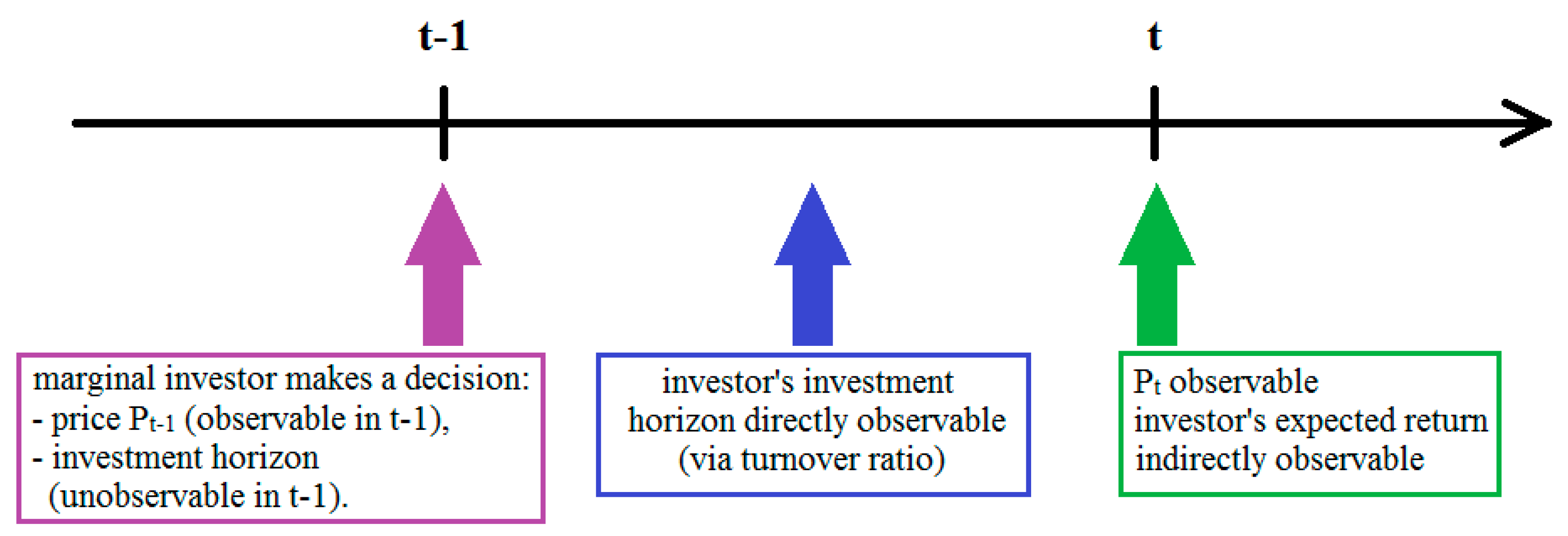
Table 1.
The results of the estimation of the models of the relationship between stock liquidity and returns.
Table 1.
The results of the estimation of the models of the relationship between stock liquidity and returns.
| Dependent Variable | M1 | M2 | M3 | M4 | M5 |
|---|---|---|---|---|---|
| Intercept | 0.116 *** | 0.054 *** | 0.058 *** | 0.081 *** | 0.097 *** |
| (10.79) | (4.967) | (5.170) | (7.347) | (8.152) | |
| lnMV | −0.019 *** | −0.019 *** | −0.017 *** | −0.016 *** | −0.020 *** |
| (11.82) | (11.51) | (10.06) | (9.647) | (11.00) | |
| BV/MV | 0.001 *** | 0.001 *** | 0.001 *** | 0.001 *** | 0.001 *** |
| (3.297) | (3.451) | (3.737) | (3.340) | (2.984) | |
| DY | 0.000 | 0.001 | 0.004 | 0.004 | −0.002 |
| (0.025) | (0.083) | (0.351) | (0.371) | (0.126) | |
| rt−12−t−1 | 0.008 *** | 0.009 *** | 0.005 ** | 0.003 | 0.004 * |
| (4.021) | (4.350) | (2.369) | (1.499) | (1.867) | |
| σ | −0.082 *** | −0.081 *** | |||
| (3.747) | (3.772) | ||||
| σε | −0.069 *** | −0.045 * | −0.053 * | ||
| (2.749) | (1.713) | (1.839) | |||
| amFHTt−1 | 2.636 *** | 2.667 *** | 2.571 *** | 2.460 *** | 2.394 *** |
| (4.164) | (4.208) | (4.066) | (4.151) | (4.227) | |
| FHTU | −0.010 | −0.001 | −0.028 | 0.086 | 0.076 |
| (0.102) | (0.010) | (0.271) | (0.835) | (0.744) | |
| Stocks effects | YES | YES | YES | YES | YES |
| Months effects | YES | YES | YES | YES | YES |
| N | 41,110 | 41,117 | 41,146 | 41,142 | 41,140 |
| R2 | 0.209 | 0.076 | 0.075 | 0.030 | 0.033 |
| F | 25.293 | 24.525 | 18.457 | 17.933 | 20.737 |
| D−W | 1.980 | 1.986 | 1.983 | 1.996 | 1.973 |
| AIC | −55,844.32 | −55,798.82 | −54,825.37 | −52,419.18 | −50,496.79 |
Table presents the estimates of the parameters of the model given with the formula (4). Dependent variables are differently determined stock returns in month t; lnMV is the natural logarithm of stock market capitalization at the end of the month t − 1; BV/MV is the ratio of last known at the end of the month t − 1 book value of equity to the market value of equity at the end of the month t − 1; DY is the last known at the end of month t − 1 dividend yield; rt−12−t−1 is the cumulated return from the months from t − 12 to t − 1; σ is the standard deviation of monthly returns in last 36 months; σε is the standard error of residuals from the pricing model; amFHT is the value of FHT measure in month t − 1 amortized by the expected holding period, approximated by the reciprocal of the turnover ratio in month t; FHTU is the residual from AR(1) model of FHT measure. t-statistics are given in the parentheses and asterisks denote the statistical significance at the 0.1 (*), 0.05 (**) and 0.01 (***) level.
Table 2.
The results of the estimation of the modified models of the relationship between stock liquidity and returns.
Table 2.
The results of the estimation of the modified models of the relationship between stock liquidity and returns.
| Dependent Variable | M1a | M1b | M1c | M1d | M1e |
|---|---|---|---|---|---|
| Intercept | 0.104 *** | 0.098 *** | 0.098 *** | 0.104 *** | 0.055 *** |
| (10.27) | (9.599) | (11.41) | (4.955) | (3.096) | |
| lnMV | −0.019 *** | −0.018 *** | −0.018 *** | −0.023 *** | −0.023 *** |
| (11.82) | (11.31) | (16.45) | (6.772) | (10.25) | |
| BV/MV | 0.001 *** | 0.001 *** | 0.001 *** | 0.001 | 0.001 *** |
| (3.297) | (3.297) | (5.291) | (0.969) | (3.577) | |
| DY | 0.000 | 0.000 | 0.003 | −0.033 | 0.004 |
| (0.025) | (0.025) | (0.274) | (1.400) | (0.379) | |
| rt−12−t−1 | 0.008 *** | 0.008 *** | 0.008 *** | −0.000 | 0.007 ** |
| (4.021) | (4.021) | (5.359) | (0.008) | (2.404) | |
| σ | −0.220 *** | −0.071 ** | |||
| (4.936) | (2.389) | ||||
| σortog_amFHT | −0.082 *** | ||||
| (3.747) | |||||
| σortog_lnMV | −0.082 *** | ||||
| (3.747) | |||||
| amFHTt−1 | 2.441 *** | 2.636 *** | 2.579 *** | 4.409 ** | 2.351 *** |
| (3.920) | (4.164) | (13.63) | (2.489) | (3.849) | |
| FHTU | −0.010 | −0.010 | 0.021 | 0.492 ** | −0.088 |
| (0.102) | (0.102) | (0.335) | (2.202) | (0.759) | |
| Stocks effects | YES | YES | YES | YES | YES |
| Months effects | YES | YES | YES | YES | YES |
| N | 41110 | 41110 | 41110 | 10455 | 30655 |
| R2 | 0.209 | 0.209 | 0.209 | 0.269 | 0.180 |
| F | 25.293 | 25.293 | 66.205 | 13.548 | 20.000 |
| D−W | 1.980 | 1.980 | 1.982 | 1.901 | 2.010 |
| AIC | −55,844.32 | −55,844.32 | −55,819.27 | −12,110.91 | −44,050.55 |
Table presents the estimates of the parameters of the modified model given with the formula (4). Dependent variables are differently determined stock returns in month t; lnMV is the natural logarithm of stock market capitalization at the end of the month t − 1; BV/MV is the ratio of last known at the end of the month t − 1 book value of equity to the market value of equity at the end of the month t − 1; DY is the last known at the end of month t − 1 dividend yield; rt−12−t−1 is the cumulated return from the months from t − 12 to t − 1; σ is the standard deviation of monthly returns in last 36 months; amFHT is the value of FHT measure in month t − 1 amortized by the expected holding period, approximated by the reciprocal of the turnover ratio in month t; FHTU is the residual from AR(1) model of FHT measure. In model M1a risk is orthogonalized vs. liquidity; in model M1b risk is orthogonalized vs. size of the company; in model M1c risk variable is omitted; model M1d is estimated using the data from the subperiod 2004–2009; model M1e is estimated using the data from the subperiod 2010–2016. t-statistics are given in the parentheses and asterisks denote the statistical significance at the 0.1 (*), 0.05 (**) and 0.01 (***) level.
Table 3.
The results of the estimation of the models of the relationship between stock liquidity and returns during the bull and bear market phases.
Table 3.
The results of the estimation of the models of the relationship between stock liquidity and returns during the bull and bear market phases.
| Dependent Variable | M6 | M7 | M8 | M9 | M10 |
|---|---|---|---|---|---|
| Intercept | 0.115 *** | 0.054 *** | 0.057 *** | 0.081 *** | 0.097 *** |
| (10.78) | (4.947) | (5.158) | (7.346) | (8.154) | |
| lnMV | −0.019 *** | −0.019 *** | −0.017 *** | −0.016 *** | −0.020 *** |
| (11.82) | (11.52) | (10.07) | (9.655) | (11.01) | |
| BV/MV | 0.001 *** | 0.001 *** | 0.001 *** | 0.001 *** | 0.0004 *** |
| (3.309) | (3.461) | (3.742) | (3.330) | (2.973) | |
| DY | 0.000 | 0.001 | 0.004 | 0.004 | −0.002 |
| (0.019) | (0.077) | (0.345) | (0.368) | (0.128) | |
| rt−12−t−1 | 0.008 *** | 0.009 *** | 0.005 ** | 0.003 | 0.004 * |
| (3.946) | (4.270) | (2.288) | (1.453) | (1.826) | |
| σ | −0.082 *** | −0.081 *** | |||
| (3.741) | (3.762) | ||||
| σε | −0.067 *** | −0.045 * | −0.053 * | ||
| (2.750) | (1.718) | (1.844) | |||
| amFHTt−1*H | 2.648 *** | 2.660 *** | 2.523 *** | 2.392 *** | 2.349 *** |
| (3.816) | (3.855) | (3.678) | (3.723) | (3.804) | |
| amFHTt−1*B | 2.501 ** | 2.653 ** | 2.851 ** | 2.919 ** | 2.690 ** |
| (2.569) | (2.426) | (2.463) | (2.410) | (2.469) | |
| FHTU*H | −0.093 | −0.081 | −0.110 | 0.037 | 0.032 |
| (0.860) | (0.733) | (0.990) | (0.340) | (0.291) | |
| FHTU*B | 0.575 ** | 0.082 ** | 0.542 ** | 0.414 * | 0.378 |
| (2.412) | (2.446) | (2.293) | (1.371) | (1.556) | |
| Stocks effects | YES | YES | YES | YES | YES |
| Months effects | YES | YES | YES | YES | YES |
| N | 41,110 | 41,117 | 41,146 | 41,142 | 41,140 |
| R2 | 0.209 | 0.076 | 0.075 | 0.030 | 0.033 |
| F | 21.107 | 20.177 | 15.852 | 14.590 | 16.516 |
| D−W | 1.981 | 1.986 | 1.983 | 1.996 | 1.973 |
| AIC | −55,853.02 | −55,807.00 | −54,833.85 | −52,420.07 | −50,496.28 |
Table presents the estimates of the parameters of the model given with the formula (5). Dependent variables are differently determined stock returns in month t; lnMV is the natural logarithm of stock market capitalization at the end of the month t − 1; BV/MV is the ratio of last known at the end of the month t − 1 book value of equity to the market value of equity at the end of the month t − 1; DY is the last known at the end of month t − 1 dividend yield; rt−12−t−1 is the cumulated return from the months from t − 12 to t − 1; σ is the standard deviation of monthly returns in last 36 months; σε is the standard error of residuals from the pricing model; amFHT is the value of FHT measure in month t − 1 amortized by the expected holding period, approximated by the reciprocal of the turnover ratio in month t; FHTU is the residual from AR(1) model of FHT measure; H is a dummy variable that equals 1 if month t is considered as belonging to the bull market and 0 otherwise; B is a dummy variable that equals 1 if month t is considered as belonging to the bear market and 0 otherwise. t-statistics are given in the parentheses and asterisks denote the statistical significance at the 0.1 (*), 0.05 (**) and 0.01 (***) level.
Table 4.
Matching diagnostic tests.
| Panel A: Pre-Match and Post-Match Propensity | ||||
| Variable | Pre-Match | Post-Match | ||
| Intercept | −1.208 * | 0.215 | ||
| (1.837) | (0.800) | |||
| lnMV | 0.143 *** | −0.016 | ||
| (3.058) | (0.8045) | |||
| BV/MV | −0.007 | −0.045 | ||
| (0.669) | (0.379) | |||
| rt−12−t−1 | 0.145 | 0.067 | ||
| (0.437) | (0.800) | |||
| σ | −2.286 | 0.640 | ||
| (0.247) | (0.810) | |||
| FHT | −1.040 | −1.812 | ||
| (0.628) | (0.667) | |||
| N | 222 | 110 | ||
| p-value of χ2 | 0.000 | 0.967 | ||
| pseudo-R2 | 0.091 | 0.006 | ||
| Panel B: Post-Matching Differences | ||||
| Variable | Treatment | Control | Difference | t-Statistic |
| lnMV | 11.193 | 11.253 | −0.06 | −0.1532 |
| .BV/MV | 1.4175 | 1.7221 | −0.3046 | −0.7701 |
| rt−12−t−1 | −0.21202 | −0.25052 | 0.0385 | 0.3831 |
| σ | 0.13734 | 0.13679 | 0.00055 | 0.0578 |
| FHT | 0.022066 | 0.024574 | −0.002508 | −0.4292 |
Panel A presents the diagnostic of the propensity score matching. Panel B presents the differences in means between treatment and control group in the post-matched sample. Dependent variable is a dummy variable that equals 1 if a firm belongs to the treatment group and 0 otherwise; lnMV is the natural logarithm of stock market capitalization at the end of the month t − 1; BV/MV is the ratio of last known at the end of the month t − 1 book value of equity to the market value of equity at the end of the month t − 1; rt−12−t−1 is the cumulated return from the months from t − 12 to t − 1; σ is the standard deviation of monthly returns in last 36 months; FHT is the value of FHT measure in month t − 1; t-statistics are given in the parentheses and asterisks denote the statistical significance at the 0.1 (*) and 0.01 (***) level.
Table 5.
The results of the difference-in-differences estimation.
| Variable | (1) | (2) | (3) |
|---|---|---|---|
| Intercept | −0.065 *** (3.142) | −0.096 (1.173) | −0.081 (1.030) |
| Aftert | 0.154 *** (4.577) | 0.148 *** (4.639) | 0.164 *** (5.066) |
| Treatmenti | 0.050 * (1.690) | 0.052 * (1.751) | 0.051 * (1.698) |
| Aftert*Treatmenti | −0.060 (1.176) | −0.053 (1.050) | −0.074 (1.523) |
| Control | NO | YES | YES |
| FHT | NO | NO | YES |
| N | 220 | 220 | 220 |
| R2 | 0.114 | 0.117 | 0.131 |
Table presents the estimates of the parameters of the model given with the formula (10). Dependent variable is stock returns in month t less risk-free return in the month t; Aftert is a dummy variable that equals one if month t is after April 2013 and 0 otherwise; Treatmenti is a dummy variable that equals 1 if firm i belongs to a treatment group and 0 if firm i belongs to a control group; control variables are the same as in Table 1. t-statistics are given in the parentheses and asterisks denote the statistical significance at the 0.1 (*) and 0.01 (***) level.
© 2020 by the author. Licensee MDPI, Basel, Switzerland. This article is an open access article distributed under the terms and conditions of the Creative Commons Attribution (CC BY) license (http://creativecommons.org/licenses/by/4.0/).
Share and Cite
MDPI and ACS Style
Stereńczak, S. State-Dependent Stock Liquidity Premium: The Case of the Warsaw Stock Exchange. Int. J. Financial Stud. 2020, 8, 13. https://0-doi-org.brum.beds.ac.uk/10.3390/ijfs8010013
AMA Style
Stereńczak S. State-Dependent Stock Liquidity Premium: The Case of the Warsaw Stock Exchange. International Journal of Financial Studies. 2020; 8(1):13. https://0-doi-org.brum.beds.ac.uk/10.3390/ijfs8010013
Chicago/Turabian StyleStereńczak, Szymon. 2020. "State-Dependent Stock Liquidity Premium: The Case of the Warsaw Stock Exchange" International Journal of Financial Studies 8, no. 1: 13. https://0-doi-org.brum.beds.ac.uk/10.3390/ijfs8010013
Note that from the first issue of 2016, this journal uses article numbers instead of page numbers. See further details here.