Improving Supply Chain Profit through Reverse Factoring: A New Multi-Suppliers Single-Vendor Joint Economic Lot Size Model


Abstract
:1. Introduction
2. Literature Review
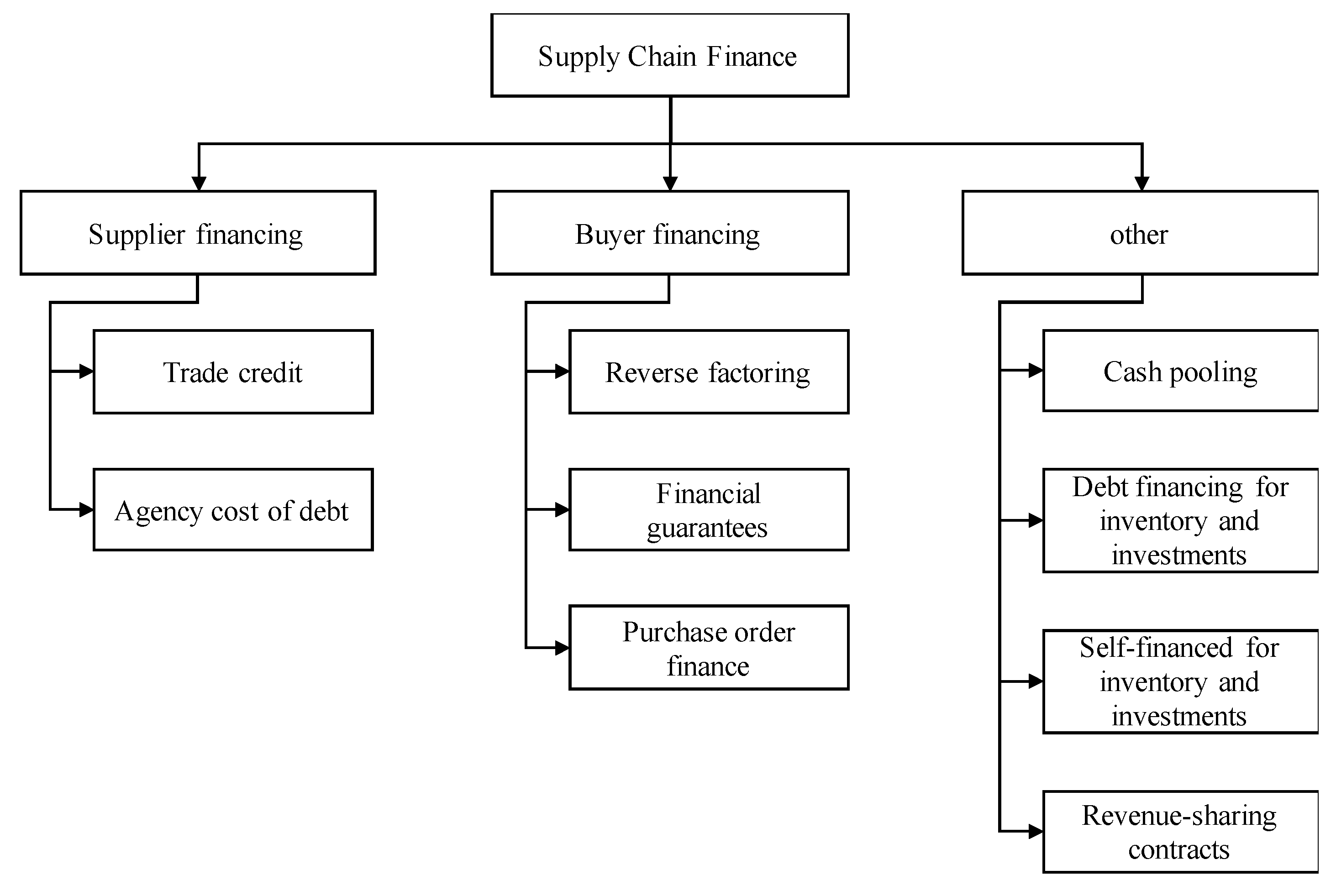
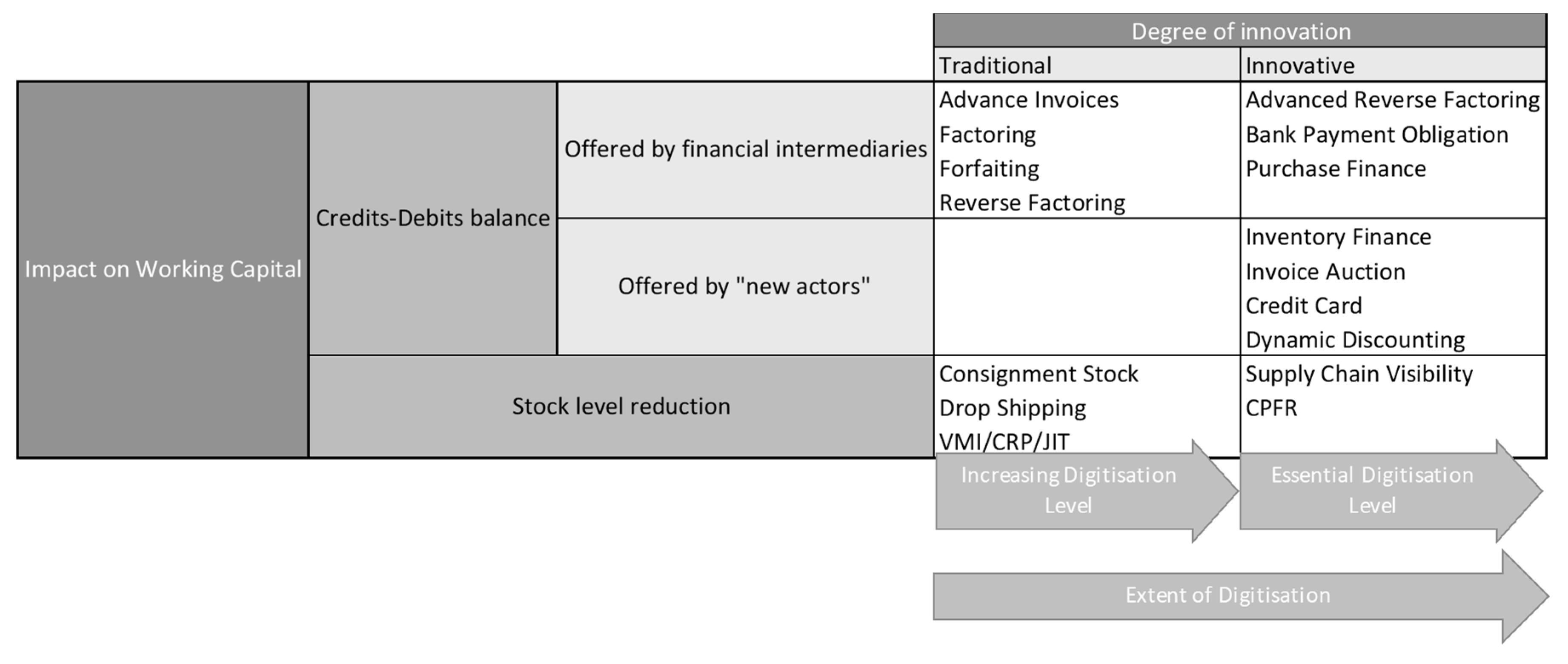
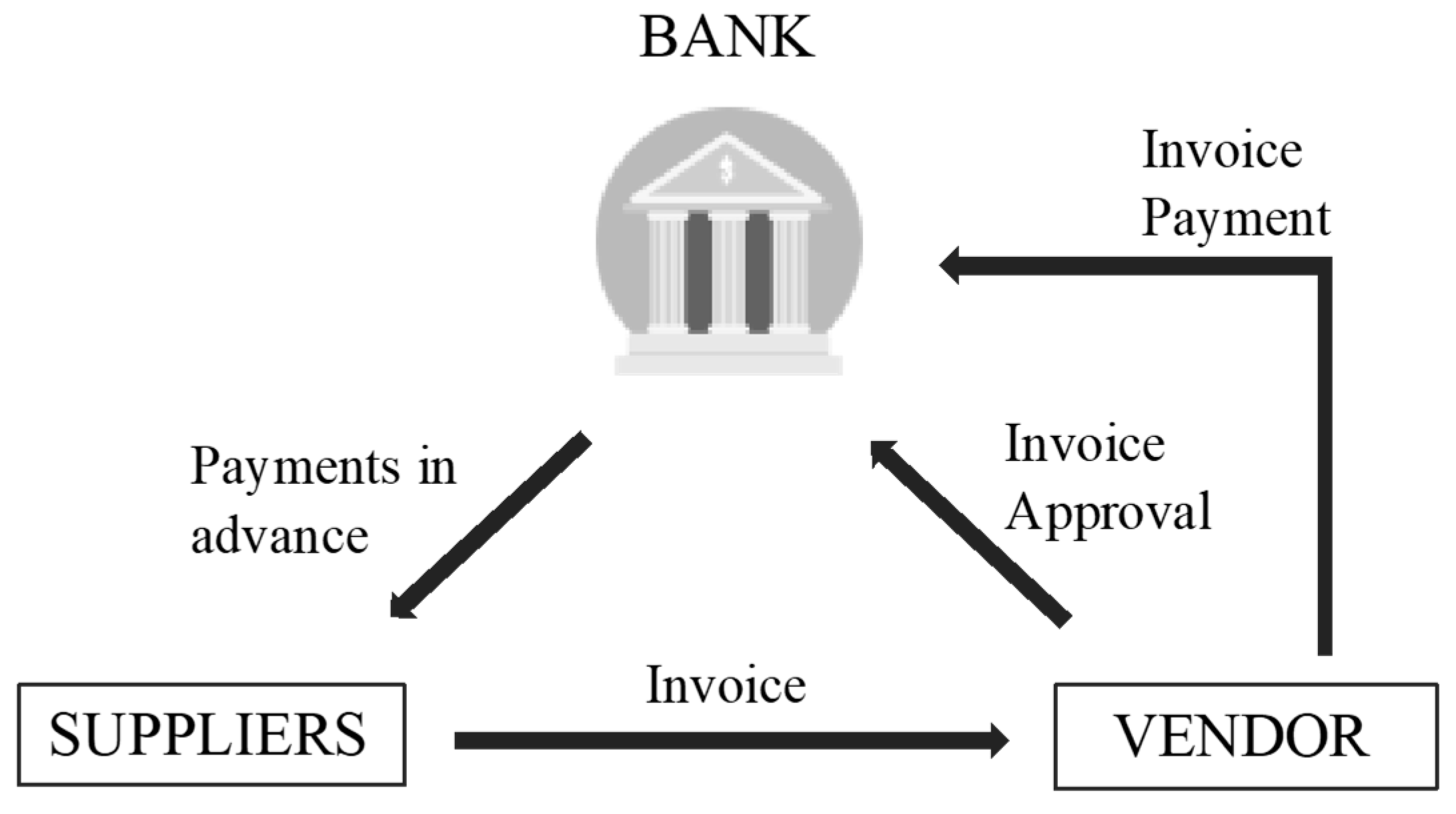
2.1. Supply Chain Finance and Reverse Factoring
2.2. Joint Economic Lot Size Models
3. Model Development
| j | part index, ; |
| number of units of part type that go into one unit of the finished product, (unit); | |
| vendor’s fixed order cost ($/order); | |
| cost for placing a purchase order for the th part ($/order); | |
| unit cost ($/unit); | |
| annual demand rate (unit/year); | |
| unit holding cost of finished product per year, consisting of two components, one physical () and the other financial () ($/unit/year); | |
| unit holding cost of part j at the vendor’s warehouse per year, consisting of two components, one physical () and the other financial () ($/unit/year); | |
| number of part types in the finished product; | |
| product unit selling price ($/unit); | |
| vendor’s production rate (unit/year); | |
| lot size quantity (unit); | |
| interest rate the bank offers to the vendor (%/year); | |
| vendor’s setup cost ($/setup). |
| s | supplier index, = 1, 2, …, ; |
| total number of suppliers; | |
| setup cost that supplier incurs when producing the th part, ($/setup); | |
| unit production cost of part for supplier ($/unit); | |
| unit holding cost per unit of time for part supplied by supplier , when there is no coordination of the financial flow. It consists of two contributions, one physical () and the other financial () ($/unit/year); | |
| holding cost per unit of time for th part supplied by supplier , consisting of two contributions, one physical () and the other financial () ($/unit/year); | |
| number of shipments for part supplier sends to the vendor; | |
| production rate of supplier for part (unit/year); | |
| supplier unit selling price for part ($/unit); | |
| interest rate the bank offers to supplier s when there is collaboration of financial flows in a supply chain (%/year); | |
| interest rate the bank offers to supplier s when there is no financial collaboration (%/year); | |
| binary parameter assuming value 1 if the part is supplied by supplier s; 0 otherwise. |
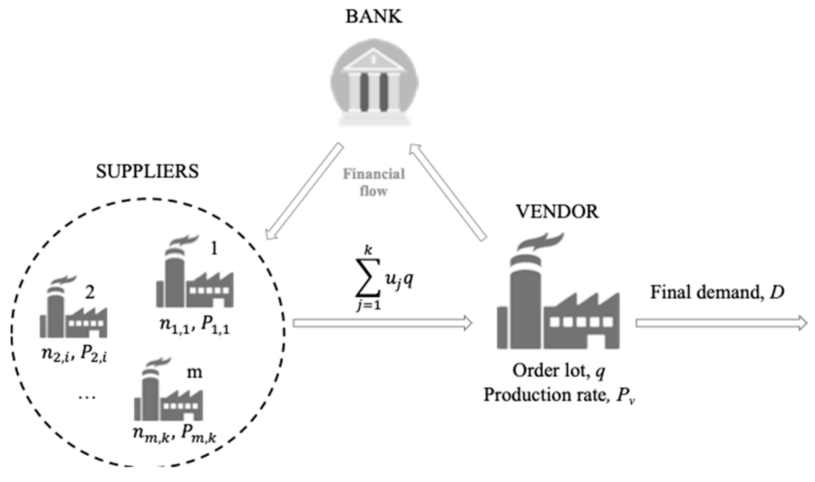
3.1. Problem Description and Assumptions
- Deterministic demand and constant over time which is lower than the production rate of the vendor ;
- The final product requires different parts;
- Shortages are not allowed;
- Lead time is assumed to be zero;
- An infinite time horizon is considered.
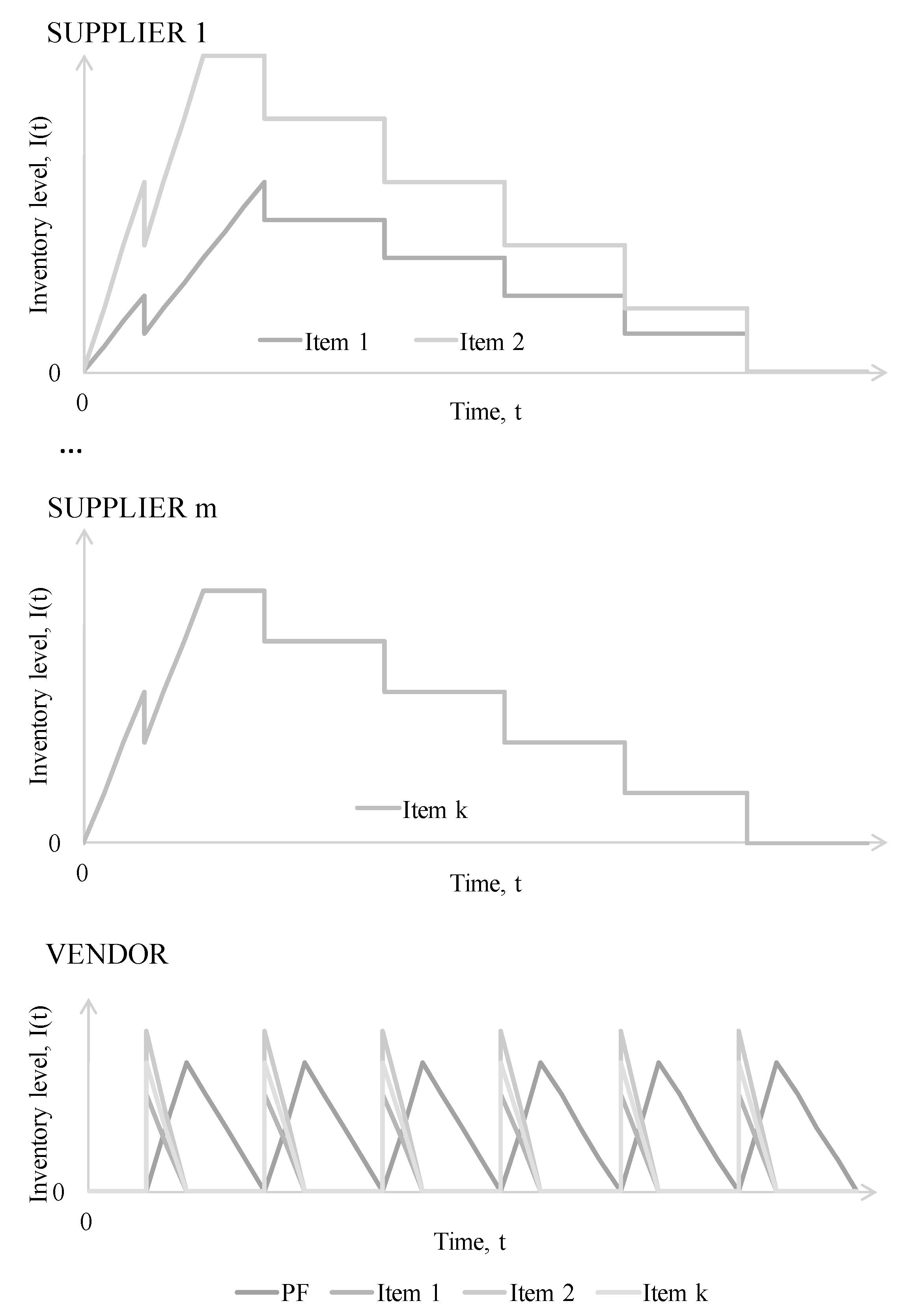
3.2. Model Development
3.2.1. The Vendor’s Annual Profit Function
3.2.2. The Suppliers’ Annual Profit Function
3.2.3. The Supply Chain’s Annual Profit Function
3.2.4. Solution Procedure
3.3. Reference Case without Reverse Factoring
4. Numerical Example
5. Summary and Conclusions
Author Contributions
Funding
Conflicts of Interest
References
- Aljazzar, Salem M., Mohamad Y. Jaber, and Lama Moussawi-Haidar. 2017. Coordination of a three-level supply chain (supplier-manufacturer-retailer) with permissible delay in payments and price discounts. Applied Mathematical Modelling 48: 289–302. [Google Scholar] [CrossRef]
- Aljazzar, Salem M., Amulya Gurtu, and Mohamad Y. Jaber. 2018. Delay-in-payments—A strategy to reduce carbon emissions from supply chains. Journal of Cleaner Production 170: 636–44. [Google Scholar] [CrossRef]
- Banerjee, Avijit. 1986. A Joint Economic-Lot-Size Model for Purchaser and Vendor. Decision Sciences 17: 292–311. [Google Scholar] [CrossRef]
- Caniato, Federico, Luca M. Gelsomino, Alessandro Perego, and Stefano Ronchi. 2016. Does finance solve the supply chain financing problem? Supply Chain Management 21: 534–49. [Google Scholar] [CrossRef]
- Dello Iacono, Umberto, Matthew Reindorp, and Nico Dellaert. 2015. Market adoption of reverse factoring. International Journal of Physical Distribution & Logistics Management 45: 286–308. [Google Scholar] [CrossRef]
- Gelsomino, Luca M., Riccardo Mangiaracina, Alessandro Perego, and Angela Tumino. 2016. Supply chain finance: A literature review. International Journal of Physical Distribution & Logistics Management 46: 348–66. [Google Scholar] [CrossRef]
- Glock, Christoph H. 2011. A multiple-vendor single-buyer integrated inventory model with a variable number of vendors. Computers & Industrial Engineering 60: 173–82. [Google Scholar] [CrossRef]
- Glock, Christoph H. 2012. The joint economic lot size problem: A review. International Journal of Production Economics 135: 671–86. [Google Scholar] [CrossRef]
- Glock, Christoph H., and Taebok Kim. 2014. Shipment consolidation in a multiple-vendor-single-buyer integrated inventory model. Computers & Industrial Engineering 70: 31–42. [Google Scholar] [CrossRef]
- Goyal, Suresh K. 1977. An integrated inventory model for a single supplier-single customer problem. International Journal of Production Research 15: 107–11. [Google Scholar] [CrossRef]
- Hofmann, Erik. 2005. Supply Chain Finance: Some conceptual insights. Logistik Management: Innovative Logistikkonzepte 80: 203–14. [Google Scholar] [CrossRef]
- Hurtrez, Nicolas, and Massimo G. S. Salvadori. 2010. Supply chain finance: From myth to reality. In McKinsey on Payments. pp. 22–28. Available online: https://www.finyear.com/attachment/252360 (accessed on 7 April 2020).
- Jaber, Mohamad Y., and Suresh K. Goyal. 2008. Coordinating a three-level supply chain with multiple suppliers, a vendor and multiple buyers. International Journal of Production Economics 116: 95–103. [Google Scholar] [CrossRef]
- Kim, Taebok, and Suresh K. Goyal. 2009. A consolidated delivery policy of multiple suppliers for a single buyer. International Journal of Procurement Management 2: 267. [Google Scholar] [CrossRef]
- Klapper, Leora. 2006. The role of factoring for financing small and medium enterprises. Journal of Banking and Finance 30: 3111–30. [Google Scholar] [CrossRef] [Green Version]
- Kraemer-Eis, Helmut, Antonia Bostari, Salome Gvetadze, Frank Lang, and Wouter Torfs. 2018. European Small Business Finance Outlook. Luxembourg: European Investment Fund. [Google Scholar]
- Lekkakos, Spyridon D., and Alejandro Serrano. 2016. Supply chain finance for small and medium sized enterprises: The case of reverse factoring. International Journal of Physical Distribution & Logistics Management 46: 367–92. [Google Scholar] [CrossRef]
- Lekkakos, Spyridon D., and Alejandro Serrano. 2017. Reverse factoring: A theory on the value of payment terms extension. Foundations and Trends in Technology, Information and Operations Management 10: 270–88. [Google Scholar] [CrossRef] [Green Version]
- Marchi, Beatrice, Jörg M. Ries, Simone Zanoni, and Christoph H. Glock. 2016. A joint economic lot size model with financial collaboration and uncertain investment opportunity. International Journal of Production Economics 176: 170–82. [Google Scholar] [CrossRef]
- Marchi, Beatrice, Simone Zanoni, Ivan Ferretti, and Lucio E. Zavanella. 2018. Stimulating Investments in Energy Efficiency through Supply Chain Integration. Energies 11: 858. [Google Scholar] [CrossRef] [Green Version]
- Marchi, Beatrice, Lucio E. Zavanella, and Simone Zanoni. 2020. Joint economic lot size models with warehouse financing and financial contracts for hedging stocks under different coordination policies. Journal of Business Economics. [Google Scholar] [CrossRef]
- Modigliani, Franco, and Merton H. Miller. 1958. The cost of capital, corporation finance, and the theory of investment. The American Economic Review 48: 261–97. [Google Scholar]
- Observatory for Supply Chain Finance. 2016. Supply Chain Finance: Opportunities in the Italian Market. Milano: Politecnico di Milano. [Google Scholar]
- Observatory for Supply Chain Finance. 2017. Supply Chain Finance: Tomorrow Is Already Here! Milano: Politecnico di Milano. [Google Scholar]
- Ouyang, Liang-Yuh, Chia-Huei Ho, and Chia-Hsien Su. 2009. An optimization approach for joint pricing and ordering problem in an integrated inventory system with order-size dependent trade credit. Computers & Industrial Engineering 57: 920–30. [Google Scholar] [CrossRef]
- Pfohl, Hans-Christian, and Moritz Gomm. 2009. Supply chain finance: Optimizing financial flows in supply chains. Journal of Logistics Research 1: 149–61. [Google Scholar] [CrossRef]
- Ramezani, Majid, Ali M. Kimiagari, and Behrooz Karimi. 2014. Closed-loop supply chain network design: A financial approach. Applied Mathematical Modelling 38: 4099–119. [Google Scholar] [CrossRef]
- Randall, Wesley S., and Martin Theodore II Farris. 2009. Supply chain financing: Using cash-to-cash variables to strengthen the supply chain. International Journal of Physical Distribution & Logistics Management 39: 669–89. [Google Scholar] [CrossRef]
- Tanrisever, Fehmi, Hande Cetinay, Matthew Reindorp, and Jan C. Fransoo. 2015. Reverse Factoring for SME Finance. SSRN. [Google Scholar] [CrossRef]
- Van Der Vliet, Kasper, Matthew J. Reindorp, and Jan C. Fransoo. 2015. The price of reverse factoring: Financing rates vs. payment delays. European Journal of Operational Research. [Google Scholar] [CrossRef] [Green Version]
- Wagner, Stephan M. 2006. A firm’s responses to deficient suppliers and competitive advantage. Journal of Business Research 59: 686–95. [Google Scholar] [CrossRef]
- Wu, Yaobin, Yingying Wang, Xun Xu, and Xiangfend Chen. 2019. Collect payment early, late, or through a third party’s reverse factoring in a supply chain. International Journal of Production Economics 218: 245–59. [Google Scholar] [CrossRef]
- Wuttke, David A., Constantin Blome, and Michael Henke. 2013. Focusing the financial flow of supply chains: An empirical investigation of financial supply chain management. International Journal of Production Economics 145: 773–89. [Google Scholar] [CrossRef]
- Wuttke, David A., Constantin Blome, Sebastian Heese, and Margarita Protopappa-Sieke. 2016. Supply chain finance: Optimal introduction and adoption decisions. International Journal of Production Economics 178: 72–81. [Google Scholar] [CrossRef]
- Xu, Xinhan, Xiangfeng Chen, Fu Jia, Steve Brown, Yu Gong, and Yifan Xu. 2018. Supply chain finance: A systematic literature review and bibliometric analysis. International Journal of Production Economics 204: 160–73. [Google Scholar] [CrossRef]
- Zhan, Jizhou, Shuting Li, and Xiangfeng Chen. 2018. The impact of financing mechanism on supply chain sustainability and efficiency. Journal of Cleaner Production 205: 407–18. [Google Scholar] [CrossRef]


| Supplier | Part | Units for One Part of Final Product () | Order Cost () | Setup Cost () | Unit Production Cost () | Production Rate () | Selling Price () | Physical Holding Cost () | ||
|---|---|---|---|---|---|---|---|---|---|---|
| 1 | 1 | 5 | 10 | 400 | 10 | 5500 | 15 | 1 | 2% | 15% |
| 1 | 2 | 2 | 10 | 400 | 20 | 3500 | 25 | 2 | ||
| 2 | 3 | 1 | 5 | 300 | 30 | 1500 | 40 | 2 | 3% | 20% |
| Case | q | n1,1 | n1,2 | n2,3 | TPV | TPS,1 | TPS,2 | TPSC | |
|---|---|---|---|---|---|---|---|---|---|
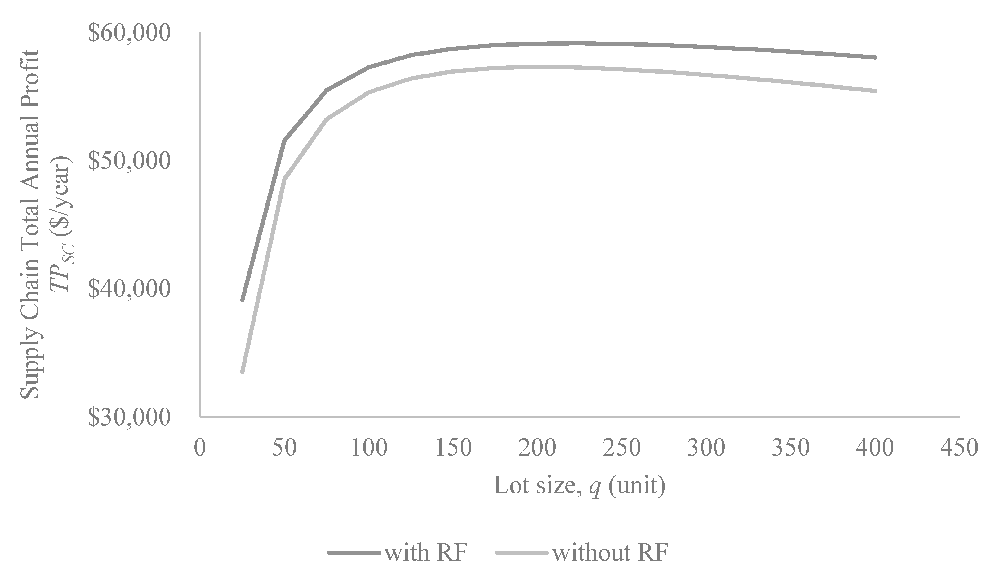
| with RF | 219 | 5 | 3 | 3 | $17,602 | $32,438 | $9120 | $59,161 | +3.23% |
| without RF | 202 | 4 | 2 | 2 | $17,849 | $31,015 | $8450 | $57,313 |
| Vendor | Supplier 1 | Supplier 2 | ||||||
|---|---|---|---|---|---|---|---|---|
| Case | SETUP COST | Order Cost | Holding Cost | Interest to the Bank | Setup Cost | Holding Cost | Setup Cost | Holding Cost |
| with RF | $915 | $572 | $585 | $327 | $976 | $1585 | $457 | $423 |
| without RF | $992 | $620 | $539 | - | $1488 | $2498 | $744 | $807 |
© 2020 by the authors. Licensee MDPI, Basel, Switzerland. This article is an open access article distributed under the terms and conditions of the Creative Commons Attribution (CC BY) license (http://creativecommons.org/licenses/by/4.0/).
Share and Cite
Marchi, B.; Zanoni, S.; Jaber, M.Y. Improving Supply Chain Profit through Reverse Factoring: A New Multi-Suppliers Single-Vendor Joint Economic Lot Size Model. Int. J. Financial Stud. 2020, 8, 23. https://0-doi-org.brum.beds.ac.uk/10.3390/ijfs8020023
Marchi B, Zanoni S, Jaber MY. Improving Supply Chain Profit through Reverse Factoring: A New Multi-Suppliers Single-Vendor Joint Economic Lot Size Model. International Journal of Financial Studies. 2020; 8(2):23. https://0-doi-org.brum.beds.ac.uk/10.3390/ijfs8020023
Chicago/Turabian StyleMarchi, Beatrice, Simone Zanoni, and Mohamad Y. Jaber. 2020. "Improving Supply Chain Profit through Reverse Factoring: A New Multi-Suppliers Single-Vendor Joint Economic Lot Size Model" International Journal of Financial Studies 8, no. 2: 23. https://0-doi-org.brum.beds.ac.uk/10.3390/ijfs8020023