Data Envelopment Analysis and Multifactor Asset Pricing Models


Department of Business Administration, Rey Juan Carlos University, 28032 Madrid, Spain
*
Author to whom correspondence should be addressed.
Int. J. Financial Stud. 2020, 8(2), 24; https://0-doi-org.brum.beds.ac.uk/10.3390/ijfs8020024
Submission received: 28 February 2020
/
Revised: 7 April 2020
/
Accepted: 13 April 2020
/
Published: 17 April 2020
Abstract
:Recent literature shows that market anomalies have significantly diminished, while research on market factors has largely improved the performance of asset pricing models. In this paper we study the extent to which data envelopment analysis (DEA) techniques can help improve the performance of multifactor models. Specifically, we test the explanatory power of the Fama and French three-factor model, combined with an additional factor based on DEA, on a sample of 2101 European equity funds, for the period from 2001 to 2016. Accordingly, we first form the fund portfolios that constitute our test assets and create the efficiency factor. Secondly, we estimate the prices of risk tied to the four factors using ordinary least squares (OLS) on a two-stage cross-sectional regression. Finally, we use the R-squared statistic estimated by generalized least squares (GLS), as well as the Gibbons Ross and Shanken test and the J-test for overidentifying restrictions in order to study the performance of the model, including and omitting the efficiency factor. The results show that the efficiency factor improves the performance of the model and reduces the pricing errors of the assets under consideration, which allows us to conclude that the efficiency index may be used as a factor in asset pricing models.
Keywords:
data envelopment analysis; Fama–French; multifactor models; mutual funds; efficiency; asset pricing; market anomaliesJEL Classification:
G12; G151. Introduction
In recent decades, research on financial market anomalies has given rise to a large number of new factors strongly related to asset returns, which have contributed to substantially improving the performance of multifactor asset pricing models. Additionally, recent research on the topic suggests that several well-known market anomalies have significantly diminished, promoting a renovated validity of the efficient market hypothesis. This fact considerably enhances the sustainability and stability of the financial system, contributing to an efficient allocation of resources. Specifically, Chordia et al. (2011) show that the intraday volatility of stock markets and the cross-sectional predictability of returns have decreased in recent years, resulting in a higher market efficiency. Consistently, Chordia et al. (2014) conclude that the greater trading activity has significantly downsized most market anomalies. Moreover, McLean and Pontiff (2016) suggest that investors learn about mispricing from academic publications, showing that portfolio returns tied to several variables useful for forecasting cross-sectional stock returns are significantly lower post-publication.
Notwithstanding the above, successful optimization techniques, such as data envelopment analysis (hereinafter DEA), have rarely been covered by the asset pricing literature, despite the fact that market factor models are directly related to efficient portfolios. Basso and Funari (2001) find that DEA is highly correlated with some classic measures of performance, such as Treynor, Sharpe and Jensen ratios. Consistently, Eling (2006) shows that under certain assumptions, the rankings provided by DEA are very close to those provided by the Sharpe ratio, while Vidal-Garcia et al. (2018) analyze the short-term market efficiency of the mutual fund industry at a global level, finding strong evidence that, in general, equity funds are close to being mean–variance efficient. According to the Roll’s Theorem (Roll 1977), if there is a risk-free rate, all efficient portfolios maximize the Sharpe ratio of the market and carry the same information about asset prices. However, the predictability pattern of stock returns (Campbell and Shiller 1988) makes it difficult to find an efficient portfolio in-sample that performs well out-of-sample when used as a risk factor. To solve this problem, the asset pricing literature has largely focused on searching for fundamental risk factors by studying a large number of market anomalies. To our best knowledge, previous research has rarely exploited the relationship that exists between DEA rankings and efficient portfolios to improve the performance of asset pricing models, but it has typically focused on using DEA to suggest specific methods for sorting mutual funds.
On this basis, in this paper we combine the Fama–French three-factor model (Fama and French 1993) with DEA tools, resulting in a new four-factor model. Particularly, we use DEA to generate a new market factor useful for determining expected excess returns, under the assumption that efficiency, as measured by DEA, can contribute to improving the performance of multifactor asset pricing models. As shown below, this allows our model to outperform the Fama–French three-factor model.
DEA methods comprise a wide range of nonparametric tools that use linear programming to capture the relationship between different inputs and outputs, in order to provide a ranking for a predetermined number of decision-making units (hereinafter DMUs). Such inputs and outputs can be flexibly chosen and can embed variables denominated in different units. Originally, DEA was conceived to evaluate the efficiency of public services, such us educational establishments (Banker et al. 1984). However, today, DEA methods are used in a wide range of activities, such as banking (Sherman and Gold 1985), the insurance industry (Fecher et al. 1993), or manufacturing (Parkan 1991). Since the 1990s, DEA tools have been used extensively to assess the efficiency of mutual funds, with Murthi el al. (1997) pioneering this research topic to a large extent.
Recent research on the financial applications of DEA largely focuses on suggesting ad hoc methods to sort mutual funds (McMullen and Strong 1998; Galagedera and Silvapulle 2002; Basso and Funari 2001; Basso and Funari 2005; Basso and Funari 2016; Zhao et al. 2011; Babalos et al. 2015; Premachandra et al. 2016; Vidal-Garcia et al. 2018; Andreu et al. 2018), hedge funds (Gregoriou and Gueyie 2003; Gregoriou et al. 2005), socially responsible mutual funds (Basso and Funari 2005; Basso and Funari 2007; Pérez-Gladish et al. 2013; Abdelsalam et al. 2014) and pension funds (Guillén 2011; Gökgöz and Çandarli 2011). However, as noted above, to our best knowledge, DEA has been rarely used to improve the performance of asset pricing models, with a few exceptions as Rubio et al. (2018) for the US market.
Regarding DEA methodology, it allows determining an efficient frontier based on a given dataset, which does not require the explicit definition of a production function, that is, a concrete function that relates inputs and outputs, substantially increasing the versatility of the model. More precisely, DEA methodology ties the resources employed by a set of DMUs with the results achieved, considering that a DMU is efficient when it is either able to produce the maximum amount of output for a certain level of input, or is able to reach a certain level of output using the least amount of input (Lovell 1993). Therefore, for a set of DMUs, the model accounts for the inputs used and the outputs produced, in order to determine the best options by comparing each DMU with all the possible linear combinations in the sample.
Accordingly, DEA provides a score equal to one for all the efficient DMUs. In this regard, a DMU is efficient when it produces a higher outcome for some output without implying a lower outcome for the rest of the outputs, and without consuming more inputs. Equivalently, a DMU is efficient when, using a lesser amount of some input but not more of the rest, it produces the same output (Charnes et al. 1981). The main strengths of the methodology include the following: (i) DEA allows considering several inputs and outputs simultaneously, (ii) it does not require an explicit definition of the relationship between inputs and outputs, (iii) each DMU is evaluated according to its relative efficiency with respect to the rest of DMUs and the linear combinations between them, (iv) inputs and outputs may be expressed in different units of measurement, and (v) the methodology allows us to sort the DMUs according to their relative efficiency.
On the other hand, factor asset pricing models use different variables—usually portfolios—to explain expected returns, in order to determine their effect on prices and to develop, among many others, performance attribution models. Although the task of finding factors with some explanatory power is challenging, nowadays there is a wide range of factors useful in asset pricing (Cochrane 2011; Feng et al. 2019). However, a lot of questions still remains to be answered, such as the hypothetical stability of the factors over time, the number of factors that are necessary to explain the cross-sectional behavior of stock returns, the best approaches to rank competing factor models and, more importantly, the definition of the underlying risk factors of special concern to investors that allow us to tie asset prices and macroeconomics.
In spite of its failure to correctly price portfolios sorted by book-to-market equity (BE/ME), the capital asset pricing model (CAPM) is one the most prominent market factor models. It assumes that expected returns are proportional to their covariances with the wealth portfolio, which is presumed to be efficient. On the other hand, the consumption capital asset pricing model (CCAPM) (Breeden 1979) assumes that expected returns are proportional to their covariance with per capita consumption growth in constant prices. (Lettau and Ludvigson 2001a; Lettau and Ludvigson 2001b) show that the consumption—wealth ratio, cay, strongly improves the explanatory power of both the CAPM and the CCAPM, as it captures part of the conditioning information available in the market.
With respect to multifactor models, the Fama–French three-factor model (Fama and French 1993) is especially remarkable given its great explanatory power and its ability to explain, among others, the value effect. On the other hand, Fama and French (2015) use operating profitability and investment to create two additional factors, which allow the authors to improve the performance of the three-factor model. Fama and French (2016) is consistent with these results. Additionally, Carhart (1997) shows that a momentum factor helps improve the performance of the Fama–French three-factor model when used as a performance attribution model. Chen et al. (2011) develop a new factor model that focuses on the production-side of the economy, with the average return of the market portfolio, the investment volume and the return-on-equity ratio as risk factors. Ammann et al. (2012) show that the explanatory power of that model is greater than that of most classic asset pricing models.
However, as mentioned above, there is not unanimity about the number of factors required to explain returns in cross-sectional models or about their concrete specification. Clarke (2014) develops a method to generate factors to price equities, while Harvey et al. (2016) collect up to 316 anomalies related to well-known factors. To the best of our knowledge, DEA methods have scarcely been used to design risk factors useful in asset pricing models, with the exception of Rubio et al. (2018), who take a different approach than the one used in this paper to study the explanatory power of DEA scores for mutual fund returns in the US market. The authors conclude that DEA scores help reduce pricing errors and have strong explanatory power.
In this paper we use the DEA methodology to form an efficiency factor, which helps us to improve the performance of the Fama–French three-factor model. As shown below, our results suggest that DEA can play an important role in generating fundamental risk factors. Furthermore, our results allow us to conclude that there is a negative relationship between efficiency and expected returns, which is coherent with the fact that the more efficient the funds, the higher their prices and, therefore, the lower their expected returns. This is consistent with McMullen and Strong (1998), who analyze 135 equity funds and conclude that the most popular funds often exhibit a poor performance.
Our study is divided into two parts. In the first part, we use the DEA methodology on a sample of 2101 European equity funds sorted into 20 size portfolios, to determine their efficiency on an annual basis, and then estimate the new efficiency factor. We calculate this factor as the difference between the returns of efficient and inefficient funds. In the second part, we test the multifactor asset pricing model on our sample, both including and omitting the efficiency factor, in order to estimate the pricing errors and compare the results. For this purpose, we first run the time-series regressions of portfolio returns on factors, which provide us with all beta coefficients, and then run the cross-sectional regression of expected returns on betas, which provide us with the prices of risk tied to each factor. We use the Gibbons et al. (1989) statistic (hereinafter GRS test) and the J-test for overidentifying restrictions to evaluate the models under consideration.
2. Data and Efficiency Analysis
We compile monthly data for 2101 Euro/Eurozone equity funds, traded in euros, for the period from January 2001 to October 2016, as provided by Morningstar. Specifically, our data series cover the following categories: Europe ex-UK Large-Cap Equity; Europe Equity-Currency Hedged; Europe ex-UK Small/Mid-Cap Equity; Europe Flex-Cap Equity; Europe Large-Cap Blend Equity; Europe Large-Cap Growth Equity; Europe Large-Cap Value Equity; Europe Mid-Cap Equity; Europe Small-Cap Equity; Eurozone Flex-Cap Equity; Eurozone Large-Cap Equity; Eurozone Mid-Cap Equity and Eurozone Small-Cap Equity. We exclude funds that invest exclusively in domestic markets in order to avoid distortions arising from risk exposures to specific areas. Thus, although the assets under management of the categories under consideration amount to 3.72 billion euros, the assets under management for the funds that constitute our sample amount to 0.547 billion euros, that is, a 14.66% of the overall sum. Regarding the number of funds, our sample comprises 2101 out of 11,641 mutual funds, that is, the 18.04% of the total funds. Table 1 shows the main summary statistics1.
It should be mentioned that throughout this paper we assume that the returns of the mutual funds under consideration are independent and identically distributed (i.i.d.), thus implicitly assuming that past performance helps us measure future performance. In any case, in the last decades, research on predictability has provided us with a wide range of variables and tools useful to forecast future returns. This fact puts into question the i.i.d. assumption and constitutes a limitation of the model. Additionally, it is worth mentioning that, in general, mutual funds provided positive returns in the period 2001–2016, despite the turbulent market environment of 2007–2008. In this framework, optimization techniques such as DEA play a key role in the task of measuring the relative performance of mutual funds. In this regard, Kapur and Timmermann (2005) study the implications on the equity premium of performance-based contracts in determining the compensation of fund managers. The authors conclude that relative performance is particularly reliable in evaluating the quality of management when the set of feet al.asible contracts is restricted, especially in bullish markets.
In general, Table 1 shows that returns exhibit a moderate volatility and a negative skewness for the period under consideration. In addition, kurtosis is positive, which means that the return data is highly concentrated around the mean.
We use the classic input-oriented DEA model with variable returns to scale (VRS). Although previous research has seldom used DEA to enhance classic asset pricing models, other literature studying the performance of mutual funds through DEA adopts extremely diverse approaches in this regard, ranging from classic constant returns to scale (hereinafter CRS), pioneered by Murthi et al. (1997), to multi-stage models, which allow us to differentiate multiple sub-processes in a sequential fashion (Premachandra et al. 2012; Zhao and Yue 2010).
In this regard, Berk and Green (2004) directly relate both the size and the performance of mutual funds, showing that the most profitable funds shall raise a large volume of funding over time, which will progressively lead them to undertake unprofitable investments, under the assumption of efficiency of the mutual fund market. This fact results in an alpha close to zero for most mutual funds, making it difficult, if not impossible, to measure the quality of management of such investments. This approach has two major implications for our model. First, near-zero alphas imply that there should be an asset pricing model which perfectly explains the expected returns of the majority of the mutual funds. As noted above, our model exploits the strong relationship between the rankings provided by DEA and the Sharpe ratio, to produce an efficiency risk factor suitable for explaining part of the cross-sectional variation of mutual fund returns. Second, since most mutual funds have a level of capital that allows them to operate optimally, we use VRS in order to account for the economies or diseconomies of scale that arise from varying the size of the fund.
In addition, in order to keep the model manageable, we use a single-stage instead a multi-stage model. In this regard, we must emphasize that our model does not require unbundling the value creation process of mutual funds, but rather provides a factor which allows us to capture the efficiency pattern of the portfolios under consideration. A single-stage model meets this requisite with a relatively low level of complexity. This is important since the increasing sophistication of DEA models can be part of the explanation for the ‘lack of visibility’ of the methodology in the financial practice (Basso and Funari 2016).
Under these assumptions, we can determine the efficiency level of any fund using linear programming, as follows:
where:
: Volume of output (1, 2... r) produced by the unit.
: Weightings, which represent the price of each output (, ... ).
: Volume of input (1, 2 ... i) consumed by the unit.
: Weightings (, ) provided by the program, which represent the price of each input and are different for each unit.
Based on the weightings (), the restrictions ensure that the result of expression (1) is less than or equal to 1 for every DMU. Therefore, according to this model, a DMU is efficient when , while every DMU that satisfies is inefficient. Since we use input-oriented DEA, the numerator of expression (1) is constant and then:
where:
: Distance from the data envelope in input units.
: Input matrix of order mxn.
: Output matrix of order sxn.
λ: Vector of weightings of order n.
: and : Vectors of inputs and outputs, respectively.
One of the main hurdles of the methodology is to determine the specific inputs and outputs of the model. Table 2 shows the variables most frequently used by the literature. However, many other variables such as costs (e.g., commissions), systemic risk (betas) or non-systemic risk (tracking error) are perfectly feasible.
As shown in Table 2, asset returns are often used as an output, although there is no unanimity on what particular class of return should be used: mean return, maximum or minimum return, etc. Remarkably, some research suggests specific measures such as the asymmetry (Wilkens and Zhu 2001), or qualitative indicators such as ethical factors (Basso and Funari 2003).
With regard to inputs, the literature on the topic explores a wide range of alternatives. Murthi et al. (1997) use the standard deviation of returns and the management fees, while Galagedera and Silvapulle (2002) use the standard deviation of returns, the distribution fees, the expense ratio and the minimum capital investment. Morey and Morey (1999) use the variance of returns, while Basso and Funari (2001) suggest using the standard deviation of returns, the beta coefficient, and the front-end and back-end loads. Glawischnig and Sommersguter-Reichmann (2010) research suggests using lower partial moments (hereinafter LPM), such as the lowest mean return, the lowest mean semivariance or the lowest mean semi-skewness. Although systemic and idiosyncratic risks are meaningful inputs which allow us to relate efficiency to a specific benchmark, they require using different benchmarks for each category of funds, which can be cumbersome. For this reason, we have ignored these variables in our study. Remarkably, Favre and Galeano (2002) develop a new version of the value-at-risk methodology, in what the authors call the modified value-at-risk (hereinafter MVaR), which uses the Cornish and Fisher (1937) methodology to compute the value-at-risk for the left tail of the distribution. This allows the authors to efficiently account for non-normally distributed returns. As shown below, the MVaR helps to largely explain the variance of the inputs under consideration in our model.
Eling (2006) suggests using either Spearman’s rank correlation or principal component analysis to determine the inputs and outputs needed to apply DEA to hedge funds. The author shows that, under certain assumptions, the rankings provided by DEA methods are very similar to those provided by the Sharpe ratio when inputs and outputs are determined by using principal component analysis. However, the disparities between these two measures increase when Spearman’s rank correlation is used. Although Spearman’s rank correlation is highly recommended when DMUs do not fit well with classic performance measures—as is the case of hedge funds—,the strong relationship between the maximum Sharpe ratio of the market—i.e., the Sharpe ratio of the mean–variance efficient portfolios—and fundamental risk factors (Roll 1977) makes us use the principal component analysis to determine inputs and outputs.
It is worth noting that this variable reduction procedure allows us to maximize the variance explained by the model and choose only those variables with the highest explanatory power. According to Adler and Golany (2002), the principal component analysis is highly recommended in DEA applications to integrate the variability of all risk and return measures. Specifically, the authors show that the principal component analysis greatly improves the discriminatory power of the model, helping us to avoid the risk that a large number of DMUs are considered efficient when the number of inputs and outputs is relatively high. This conclusion is consistent with those of Zhu (1998), Premachandra (2001) and Serrano Cinca and Mar Molinero (2004). Table 3 shows the results of our principal components analysis.
Regarding inputs, lower partial moments order 2 (LPM2) is the variable with the greatest effect on component 1 (factor loading of 0.993), while MVaR 95% is the most relevant variable for component 2 (factor loading of 0.997). Remarkably, components 1 and 2 explain the 84.94% of the variance of the inputs. Regarding outputs, higher partial moments order 1 (HPM1) (factor loading of 0.98 for component 1) and skewness (factor loading of 0.982 for component 2) are the most important variables in the principal components analysis. As shown, components 1 and 2 explain the 78.41% of the variance of the outputs.
Once the inputs and outputs are determined, we sort the 2101 funds that constitute our sample into 20 size portfolios. Specifically, at the end of each year, we use the volume of assets under management to sort funds into percentiles. This allows us to determine monthly mean returns for 20 equal-weighted portfolios for the year following the portfolio formation period. Hereafter, portfolio 1 comprises the smallest funds and portfolio 20 comprises the largest ones.
Table 4 shows the summary statistics of our 20 portfolios, for the period from January 2001 to October 20162. As shown, in general, small funds provide higher returns than large funds, but they also have higher standard deviations. Additionally, our results seem to reject normality of portfolio returns, revealing negative skewness in all cases.
We use the methodology described above to estimate the DEA score of our 20 portfolios for each year in our time interval. Table 5 shows the average results3. These results suggest that small funds are more efficient than large funds, except in the case of the P18 portfolio, which exhibits a high DEA score despite its large size. Consequently, small size funds tend to be more efficient and, in general, provide higher returns.
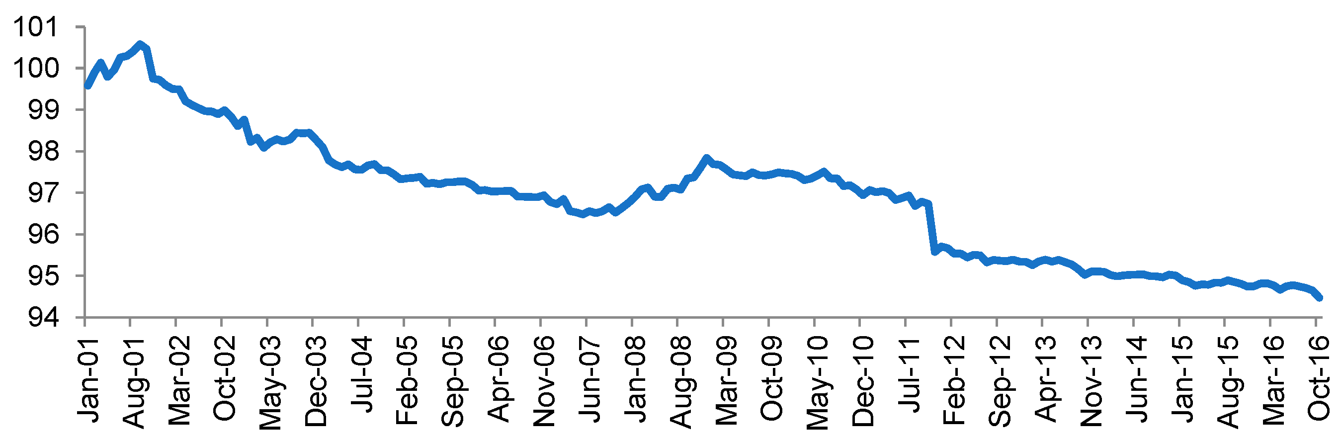
These results allow us to sort our sample into efficient portfolios (DEA score equal to one) and inefficient portfolios (DEA score less than one), for each year. Accordingly, we generate the efficiency factor for each period by determining the difference between the average return of the efficient and inefficient portfolios. Figure 1 shows the pattern of the efficiency factor over time, with base 100 and a logarithm scale. As shown, for the period 2007–2009—the crisis period—the efficiency of mutual funds increases significantly.
3. Multifactor Asset Pricing Models Results
In this section we test the Fama–French three-factor model, both including and omitting the new efficiency factor, in order to check the impact of this new factor on the pricing errors of the model. We use the two-pass cross-sectional regression (CSR) method to estimate all parameters. Specifically, we first estimate all betas for our test assets using time-series regressions, and then run the cross-section regression of expected returns on betas to determine the prices of risk. We use the generalized method of moments (GMM) to correct the standard errors for cross-sectional autocorrelation and for the fact that betas are generated regressors. Additionally, we use both the GRS test and the J-test for overidentifying restrictions to test the null of asset pricing errors equal to zero.
The time-series regression function of the Fama–French three-factor model, including our new efficiency factor, can be written as follows:
where is the return of the portfolio i for the period t, is the risk-free rate, is the market portfolio return minus the risk-free rate, and are the size and value factors, respectively, according to the Fama and French (1993) model, is the new efficiency factor, is the intercept and is the error term.
The slopes of expression (3) measure the exposure of the portfolios to each factor, while the intercept captures the average return provided by each portfolio with respect to an equivalent passive investment. Thus, in general, a positive indicates that the fund is well managed, and vice versa. Logically, when the asset pricing model perfectly fits expected returns, all intercepts are zero.
Table A1 of the Appendix shows the time-series regression estimates for all portfolios under consideration, as well as the correlations between the factors, while Table A2 shows the same results for the classic Fama–French three-factor model4. We use OLS to estimate all parameters. As shown in Table 1, RMRF is negatively correlated with the other factors. Conversely, SMB and HML are positive correlated, and the same is true for SMB and DEA. As shown, SMB and HML have a correlation close to zero, while DEA and HML have a correlation coefficient of 0.425.
Regarding to the new efficiency factor, it is remarkable that: (i) there is an inverse relation between efficiency and the market return, (ii) efficiency and size factors move in the same direction, and (iii) the efficiency factor and HML have a strong positive correlation.
As shown in Table A1, betas on RMRF are strongly significant for the 20 portfolios, with an average value of 0.71. Conversely, betas on the size factor are not significant except for the case of the four largest portfolios. Therefore, the bigger the size, the more important this factor becomes, having a negative correlation with the profitability of the portfolio. In our sample, HML has a poor explanatory power, with betas that are significant in only 6 out to 20 portfolios. With respect to the new efficiency factor, despite most betas being close to zero, they are significant in 17 portfolios, which supports its validity.
With regard to the three-factor model as shown in Table A2, RMRF is strongly significant in all cases, while the size factor is not significant, except for the case of the two largest portfolios. HML is significant in 15 out to 20 portfolios, with an average value of −0.17.
As noted above, in order to study the influence of each factor on the expected portfolio returns, we run the following cross-sectional regression of expected returns on betas:
where is the price of risk for the factor j.
Table 6 shows that the prices of risk of all factors are positive with the exception of the efficiency factor, which is consistent with the mean of this factor that amounts to −0.0178. This fact allows us to conclude that the efficiency factor behaves inversely to performance, that is, the least efficient funds are those that have higher expected returns. This relation is consistent with the mechanics of other well-known factors such as SMB or HML. Specifically, these results suggest that the more efficient an investment is, the higher its price and, consequently, the lower the expected return. As in other tests of the Fama–French model in the literature, none of the factors is statistically significant except HML. However, this fact does not reduce the economic significance of the model.
The results provided by the R-squared statistics, the GRS test and the J-test confirm the explanatory power of the model and, more particularly, the efficiency factor. We estimate R-squared statistics using both OLS and GLS. As Lewellen et al. (2010) demonstrate, the GLS R-squared statistic constitutes a stronger hurdle for the model, since its value depends entirely on the theoretical efficiency of the set of factors. Table 6 shows that the GLS R-squared statistic of the three-factor model amounts to 59.4%, while it rises to 70.8% when we add the efficiency factor, which confirms the explanatory power of this factor. The GRS test and the J-test fail to reject the models. Specifically, for the three-factor model, the GRS and J-test statistics amounts to 7.98 and 7.057, respectively, while such statistics fall to 7.222 and 6.698 when we add the efficiency factor. Therefore, these results allow us to conclude that the efficiency factor reduces the probability of rejecting the model.
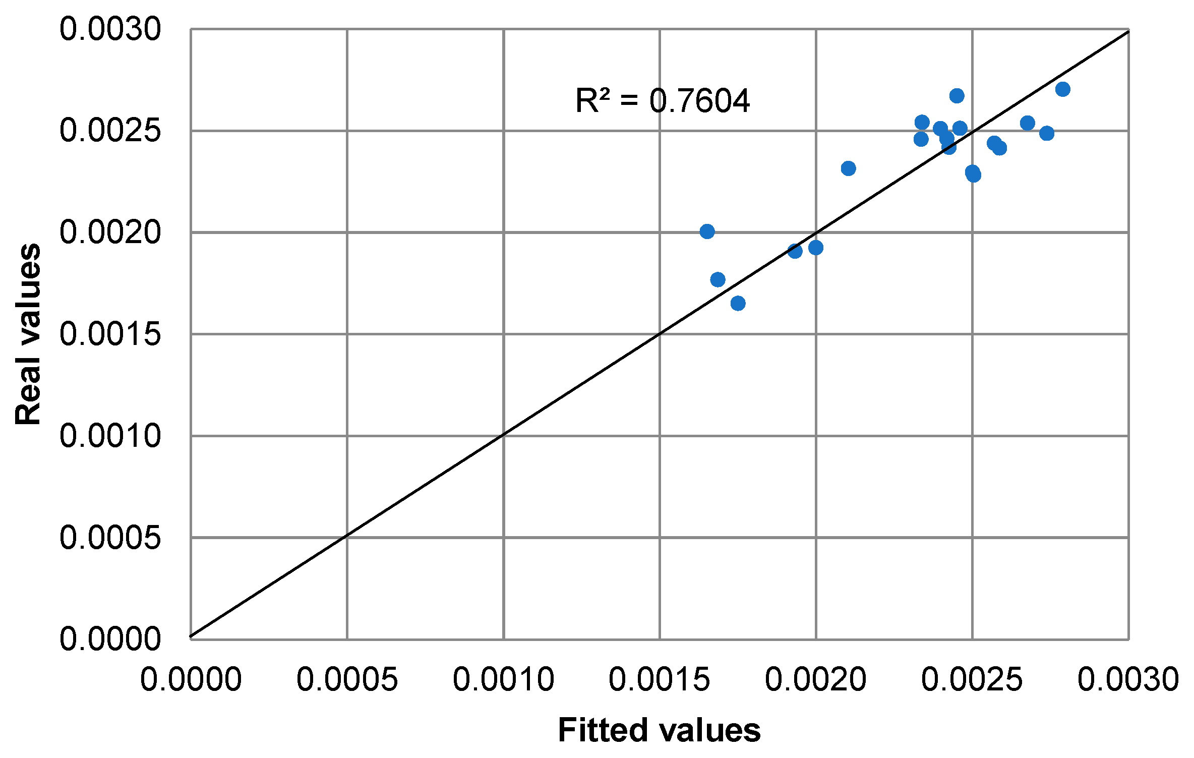
Figure 2 and Figure 3 show that, in general, the results provided by the model are close to the 45º axis, which confirm the goodness of fit. As shown, with a GLS R-squared statistic of 70.8%, the four-factor model provides better results, which confirm that the efficiency factor has strong pricing implications for asset pricing models.
4. Discussion and Conclusions
In this paper we use a sample of 2101 European equity funds sorted on 20 size portfolios, in order to test the impact of using DEA methodology to form a portfolio that can be used as a factor in asset pricing models, and more particularly, in the Fama–French three-factor model. The efficiency in DEA terms has rarely been studied in the framework of asset pricing models, in spite of its high potential, with a few exceptions as Rubio et al. (2018). These authors study the explanatory power of DEA scores for mutual fund returns in the US market, concluding that DEA scores help reduce pricing errors and improve forecasting models.
Consequently, every year we calculate the DEA score of the 20 portfolios into consideration, in order to build a portfolio with a long position in efficient portfolios and a short position in inefficient ones. We test the Fama–French three-factor model both including and omitting the new efficiency factor. In all cases, the GRS test and the J-test fail to reject the models, while OLS and GLS R-squared statistics confirm the explanatory power of the new efficiency factor.
Both the price of risk of the efficiency factor and the mean of this factor confirm that the higher the efficiency, the lower the expected return. This fact seems to confirm the paradox of ‘the good stock, the bad investment’, as the most efficient funds shall have the highest prices and, consequently, the lowest expected returns.
Our results have three main implications for asset pricing research. First, DEA can be a powerful tool for forecasting asset returns. On the basis of the intertemporal-CAPM (ICAPM), any state variable describing shifts on the investment opportunity set of investors can be used as a factor in multifactor asset pricing models. These state variables must describe the conditional distribution of asset returns and, consequently, must help to forecast returns or macroeconomic series. In this framework, our efficiency factor operates as a mimicking portfolio of some risk factor of special concern to investors and, therefore, can be useful to forecast returns and future levels of efficiency. Accordingly, DEA can provide new insight in creating scaled portfolios and factors in conditional models.
Second, our research introduces an innovative and unexplored approach to create new factors that may be exploitable in asset pricing models. Typically, market factors are related to specific strategies that constitute anomalies in classic asset pricing models. By contrast, our approach allows us to generate factors not directly related to any anomaly, but related to the inputs and outputs selected in the analysis, which allows us a better control of the process. However, further research on the robustness of the efficiency factor to changes in the inputs and outputs is necessary.
Third, our methodology expands the number of factors available for performance attribution models. Specifically, efficiency factors can help to better measure alphas and quantify the fraction of the returns directly attributable to efficiency risk exposure. Moreover, DEA allows associating the performance of the mutual funds with the inputs used to estimate the DEA score.
Notwithstanding the above, our results raise several challenges that must be addressed in depth in future research. First, although the DEA factor contributes to improve the performance of the Fama–French three-factor model, the pricing errors provided by the four-factor model are far from being zero for most portfolios. Further research on the explanatory power of risk factors omitted in our analysis is necessary. In this respect, Cao et al. (2018) conduct a research on the Chinese stock market to determine to what extent the negative correlation between idiosyncratic volatility and stock returns can be explained by different key theories suggested by the literature. The authors follow a methodology based on different conditionally sorted portfolios and the monotonic relation between anomalies and stock returns to test whether the sensitivity of alphas to idiosyncratic volatility is statistically significant. For this purpose, the authors sort portfolios using a large number of variables, such as momentum, liquidity, capital gains overhang or turnover. We believe that future research should use this approach to supplement our model, as it can contribute to finding potential patterns in pricing errors.
Second, we believe that future research should implement more sophisticated methods to form fund portfolios in order to study to what extent our results are sensitive to the portfolio formation procedure. In this regard, Pätäri et al. (2012) suggest an innovative approach that use DEA to integrate value investing and momentum investing strategies. The authors use different versions of DEA models, ranging from super-efficiency to cross-efficiency methods to study the capability of DEA tools in order to improve the performance of equity portfolios. The majority of the alphas provided by our four-factor model are relatively small, allowing the model to correctly price most portfolios under consideration. However, future research should study whether the value creation arising from the portfolio formation process, as suggested by Pätäri et al. (2012), increases pricing errors.
Third, sustainable investing is becoming an important issue across global financial markets, so research on the performance of these assets is essential in order to achieve conclusions about their similarities and differences compared to classic mutual funds. In this regard, Durán-Santomil et al. (2019) study the effects of socially responsible investments (SRI) on the performance of European equity funds. Accordingly, we suggest deepening this relationship, using DEA to determine to what extent there is a large number of funds that are not declared sustainable, but that behave as if they were, and vice versa.
Finally, it is necessary to explicitly relate the efficiency in DEA terms with the classic efficiency in the mean–variance space, as this is a key element in asset pricing problems, given the relationship between mean–variance frontiers, beta models and discount factors (Cochrane 2005).
Author Contributions
The authors equally contributed to the development of this research. Conceptualization P.S.-T., A.B.A.-C. and J.R.-S. Data curation: P.S.-T. Formal analysis: P.S.-T., A.B.A.-C. and J.R.-S. Investigation: P.S.-T., A.B.A.-C. and J.R.-S. Methodology: P.S.-T., A.B.A.-C. and J.R.-S. Project administration: A.B.A.-C. and J.R.-S. Resources: A.B.A.-C. and J.R.-S. Software: P.S.-T. and J.R.-S. Supervision: A.B.A.-C. and J.R.-S. Validation: A.B.A.-C. and J.R-S. Visualization: A.B.A.-C. and J.R.-S. Writing—original draft: P.S.-T., A.B.A.-C. and J.R.-S. Writing—review and editing: A.B.A.-C. and J.R.-S. All authors have read and agreed to the published version of the manuscript.
Funding
This research received no external funding.
Conflicts of Interest
The authors declare no conflict of interest.
Appendix A

Table A1.
Time-series regression results for the four-factor model 1.
| Panel A | ||||||
| αi | βiRMRF | βiSMB | βiHML | βiDEA | R2 | |
| P1 | 0.00001 | 0.72500 | −0.03498 | −0.13344 | −0.00672 | 0.699 |
| 0.008 | 18.462 * | −0.362 | −1.559 | −0.904 | ||
| P2 | −0.00015 | 0.68950 | 0.03730 | −0.10205 | −0.00577 | 0.709 |
| −0.082 | 18.969 * | 0.417 | −1.288 | −0.840 | ||
| P3 | −0.00068 | 0.73318 | −0.00146 | −0.23141 | −0.01505 | 0.729 |
| −0.366 | 19.667 * | −0.015 | −2.849 * | −2.136 | ||
| P4 | −0.00027 | 0.66036 | 0.02814 | −0.07859 | −0.01493 | 0.730 |
| −0.159 | 19.370 * | 0.335 | −1.058 | −2.316 * | ||
| P5 | −0.00028 | 0.69663 | −0.01145 | −0.09888 | −0.01045 | 0.720 |
| −0.155 | 19.157 * | −0.128 | −1.248 | −1.520 | ||
| P6 | −0.00018 | 0.70371 | −0.04959 | −0.11263 | −0.01544 | 0.748 |
| −0.104 | 20.318 * | −0.582 | −1.492 | −2.359 * | ||
| P7 | 0.00001 | 0.69221 | −0.02033 | −0.11473 | −0.01373 | 0.743 |
| 0.003 | 20.205 * | −0.241 | −1.537 | −2.119 * | ||
| P8 | −0.00029 | 0.69893 | −0.05205 | −0.11688 | −0.01911 | 0.757 |
| −0.169 | 20.608 * | −0.623 | −1.581 | −2.981 * | ||
| P9 | 0.00009 | 0.68879 | −0.08391 | −0.08150 | −0.01565 | 0.742 |
| 0.054 | 19.869 * | −0.983 | −1.079 | −2.388 * | ||
| P10 | −0.00036 | 0.72169 | −0.12809 | −0.11672 | −0.01475 | 0.749 |
| −0.203 | 20.339 * | −1.467 | −1.509 | −2.199 * | ||
| P11 | −0.00016 | 0.72227 | −0.10462 | −0.09785 | −0.01301 | 0.745 |
| −0.091 | 20.181 * | −1.188 | −1.255 | −1.922 ** | ||
| P12 | −0.00012 | 0.71936 | −0.03390 | −0.14850 | −0.02247 | 0.763 |
| −0.067 | 20.862 | −0.399 | −1.976 * | −3.448 * | ||
| P13 | −0.00052 | 0.72088 | −0.04617 | −0.21277 | −0.02463 | 0.755 |
| −0.295 | 20.351 * | −0.529 | −2.757 * | −3.678 * | ||
| P14 | −0.00005 | 0.71099 | −0.05945 | −0.14467 | −0.01921 | 0.745 |
| −0.025 | 20.019 * | −0.680 | −1.869 ** | −2.861 * | ||
| P15 | 0.00022 | 0.68800 | −0.08782 | −0.07565 | −0.01133 | 0.745 |
| 0.127 | 19.733 * | −1.023 | −0.995 | −1.719 ** | ||
| P16 | −0.00001 | 0.71240 | −0.00394 | −0.11358 | −0.01885 | 0.735 |
| −0.004 | 20.874 * | −0.047 | −1.527 | −2.922 * | ||
| P17 | −0.00010 | 0.70986 | −0.14161 | −0.10103 | −0.01922 | 0.760 |
| −0.057 | 20.603 * | −1.670 ** | −1.345 | −2.951 * | ||
| P18 | −0.00068 | 0.72072 | −0.15536 | −0.15191 | −0.01856 | 0.760 |
| −0.383 | 20.382 * | −1.785 ** | −1.971 | −2.777 * | ||
| P19 | −0.00026 | 0.69972 | −0.16780 | −0.14017 | −0.01822 | 0.753 |
| −0.152 | 20.940 * | −2.0410 * | −1.925 ** | −2.885 * | ||
| P20 | −0.00034 | 0.71460 | −0.20556 | −0.16629 | −0.01597 | 0.764 |
| −0.210 | 22.295 * | −2.606 * | −2.381 * | −2.636 * | ||
| Panel B | ||||||
| RMRF | SMB | HML | DEA | |||
| RM−RF | 1 | −0.098 | 0.288 | −0.294 | ||
| SMB | 1.000 | 0.048 | −0.071 | |||
| HML | 1.000 | 0.114 | ||||
| DEA | 1 |
1 Panel A shows the results of the time-series regressions of the returns of 20 size portfolios of European equity mutual funds, on the three classic factors of Fama–French—RMRF, SMB and HML—and the new efficiency factor. Panel B shows the correlations between these factors. Significance: * 0.05, ** 0.01.
Table A2.
Time-series regression results for the three-factor model 1.
| αi | βiRMRF | βiSMB | βiHML | R2 | |
|---|---|---|---|---|---|
| P1 | 0.00013 | 0.73767 | −0.02400 | −0.15109 | 0.698 |
| 0.064 | 20.1171 * | −0.250 | −1.814 ** | ||
| P2 | −0.00005 | 0.70039 | 0.04674 | −0.11722 | 0.708 |
| −0.030 | 20.6417 * | 0.527 | −1.521 | ||
| P3 | −0.00044 | 0.76157 | 0.02316 | −0.27095 | 0.722 |
| −0.232 | 21.6597 * | 0.252 | −3.3939 * | ||
| P4 | −0.00003 | 0.68852 | 0.05255 | −0.11780 | 0.722 |
| −0.016 | 21.3683 * | 0.624 | −1.610 | ||
| P5 | −0.00011 | 0.71635 | 0.00564 | −0.12634 | 0.716 |
| −0.061 | 21.0124 * | 0.063 | −1.632 | ||
| P6 | 0.00007 | 0.73284 | −0.02434 | −0.15320 | 0.740 |
| 0.041 | 22.3759 * | −0.284 | −2.0601 * | ||
| P7 | 0.00023 | 0.71810 | 0.00212 | −0.15079 | 0.737 |
| 0.134 | 22.2287 * | 0.025 | −2.0557 * | ||
| P8 | 0.00003 | 0.73499 | −0.02080 | −0.16710 | 0.745 |
| 0.015 | 22.7194 * | −0.246 | −2.2748 * | ||
| P9 | 0.00035 | 0.71832 | −0.05832 | −0.12262 | 0.734 |
| 0.200 | 21.9044 * | −0.681 | −1.647 | ||
| P10 | −0.00012 | 0.74952 | −0.10397 | −0.15548 | 0.743 |
| −0.066 | 22.3809 * | −1.188 | −2.0447 * | ||
| P11 | 0.00005 | 0.74680 | −0.08335 | −0.13202 | 0.740 |
| 0.028 | 22.1758 * | −0.947 | −1.7265 ** | ||
| P12 | 0.00025 | 0.76175 | 0.00285 | −0.20753 | 0.748 |
| 0.142 | 22.9835 * | 0.033 | −2.7578 * | ||
| P13 | −0.00012 | 0.76735 | −0.00590 | −0.27747 | 0.737 |
| −0.066 | 22.4433 * | −0.066 | −3.5742 * | ||
| P14 | 0.00027 | 0.74723 | −0.02803 | −0.19514 | 0.734 |
| 0.149 | 22.0979 * | −0.317 | −2.5416 * | ||
| P15 | 0.00041 | 0.70938 | −0.06928 | −0.10543 | 0.731 |
| 0.234 | 21.6647 * | −0.810 | −1.418 | ||
| P16 | 0.00030 | 0.74796 | 0.02689 | −0.16310 | 0.749 |
| 0.174 | 22.9976 * | 0.316 | −2.2087 * | ||
| P17 | 0.00022 | 0.74611 | −0.11018 | −0.15152 | 0.749 |
| 0.123 | 22.7135 * | −1.284 | −2.0314 * | ||
| P18 | −0.00037 | 0.75574 | −0.12501 | −0.20067 | 0.743 |
| −0.208 | 22.4747 * | −1.423 | −2.6282 * | ||
| P19 | 0.00004 | 0.73410 | −0.13801 | −0.18804 | 0.754 |
| 0.025 | 23.0654 * | −1.6590 ** | −2.6021 * | ||
| P20 | −0.00008 | 0.74473 | −0.17945 | −0.20825 | 0.776 |
| −0.047 | 24.4820 * | −2.2578 * | −3.0151 * |
1 Panel A shows the results of the time-series regressions of the returns of 20 size portfolios of European equity mutual funds, on the three classic factors of Fama–French, RMRF, SMB, and HML. Significance: * 0.05, ** 0.01.
References
- Abdelsalam, Omneya, Meryem Duygun Fethi, Juan Carlos Matallín, and Emili Tortosa-Ausina. 2014. On the Comparative Performance of Socially Responsible and Islamic Mutual Funds. Journal of Economic Behavior and Organization 7: 108–28. [Google Scholar] [CrossRef] [Green Version]
- Adler, Nicole, and Boaz Golany. 2002. Including Principal Component Weights to Improve Discrimination in Data Envelopment Analysis. Journal of the Operational Research Society 53: 985–91. [Google Scholar] [CrossRef]
- Ammann, Manuel, Sandro Odoni, and David Oesch. 2012. An Alternative Three-factor Model for International Markets: Evidence from the European Monetary Union. Journal of Banking and Finance 36: 1857–64. [Google Scholar] [CrossRef] [Green Version]
- Andreu, Laura, Miguel Serrano, and Luis Vicente. 2018. Efficiency of mutual fund managers: A slacks-based manager efficiency index. European Journal of Operational Research 273: 1180–93. [Google Scholar] [CrossRef] [Green Version]
- Babalos, Vassilios, Michael Doumpos, Nikolaos Philippas, and Constantin Zopounidis. 2015. Towards a Holistic Approach for Mutual Fund Performance Appraisal. Computational Economics 46: 35–53. [Google Scholar] [CrossRef]
- Banker, Rajiv D., Abraham Charnes, and William W. Cooper. 1984. Models for Estimating Technical and Scale Inefficiencies in Data Envelopment Analysis. Management Science 30: 1078–92. [Google Scholar] [CrossRef] [Green Version]
- Basso, Antonella, and Stefania Funari. 2001. A Data Envelopment Analysis Approach to Measure the Mutual Fund Performance. European Journal of Operational Research 135: 477–92. [Google Scholar] [CrossRef]
- Basso, Antonella, and Stefania Funari. 2003. Measuring the Performance of Ethical Mutual Funds: A DEA Approach. Journal of the Operational Research Society 54: 521–31. [Google Scholar] [CrossRef]
- Basso, Antonella, and Stefania Funari. 2005. A Generalized Performance Attribution Technique for Mutual Funds. Central European Journal of Operations Research 13: 65–84. [Google Scholar]
- Basso, Antonella, and Stefania Funari. 2007. DEA Models for Ethical and non Ethical Mutual Funds with Negative Data. Mathematics and Methods in Economics Finance 2: 21–40. [Google Scholar]
- Basso, Antonella, and Stefania Funari. 2016. DEA Performance Assessment of Mutual Funds in Data Envelopment Analysis. In A Handbook of Empirical Studies and Applications. Edited by Joe Zhu. New York: Springer, pp. 229–88. [Google Scholar]
- Berk, Jonathan B., and Richard C. Green. 2004. Mutual Fund Flows and Performance in Rational Markets. Journal of Political Economy 112: 1269–95. [Google Scholar] [CrossRef]
- Breeden, Douglas T. 1979. An Intertemporal Asset Pricing Model with Stochastic Consumption and Investment Opportunities. Journal of Financial Economics 7: 265–96. [Google Scholar] [CrossRef]
- Campbell, John Y., and Robert J. Shiller. 1988. The Dividend-Price Ratio and Expectations of Future Dividends and Discount Factors. Review of Financial Studies 1: 195–227. [Google Scholar] [CrossRef] [Green Version]
- Cao, Zhiguang, Stephen Satchell, P. Joakim Westerholm, and Hui Henry Zhang. 2018. The Idiosyncratic Volatility Anomaly and the Resale Option in Chinese Stock Markets. Available online: https://ssrn.com/abstract=3274652 (accessed on 3 April 2020).
- Carhart, Mark. M. 1997. On Persistence in Mutual Fund Performance. Journal of Finance 52: 57–82. [Google Scholar] [CrossRef]
- Charnes, Abraham, William W. Cooper, and Edward Rhodes. 1981. Evaluating Program and Managerial Efficiency: An Application of Data Envelopment Analysis to Program Follow Through. Managerial Science 27: 668–97. [Google Scholar] [CrossRef]
- Chen, Long, Robert Novy-Marx, and Lu Zhang. 2011. An Alternative Three-Factor Model. Available online: https://ssrn.com/abstract=1418117 (accessed on 28 June 2019).
- Chordia, Tarun, Avanidhar Subrahmanyam, and Qing Tong. 2014. Have capital market anomalies attenuated in the recent era of high liquidity and trading activity? Journal of Accounting and Economics 58: 41–58. [Google Scholar] [CrossRef]
- Chordia, Tarun, Richard Roll, and Avanidhar Subrahmanyam. 2011. Recent trends in trading activity and market quality. Journal of Financial Economics 101: 243–63. [Google Scholar] [CrossRef] [Green Version]
- Clarke, Charles. 2014. The Level, Slope and Curve Factor Model for Stocks. Available online: https://papers.ssrn.com/sol3/papers.cfm?abstract_id=2526435 (accessed on 17 November 2018).
- Cochrane, John H. 2011. Presidential Address: Discount Rates. Journal of Finance 66: 1047–1108. [Google Scholar] [CrossRef] [Green Version]
- Cochrane, John. H. 2005. Asset Pricing, Revised ed. Princeton: Princeton University Press. [Google Scholar]
- Cornish, Edmund A., and Ronald A. Fisher. 1937. Moments and Cumulants in the Specification of Distributions. Review of the International Statistical Institute 4: 307–20. [Google Scholar] [CrossRef] [Green Version]
- Durán-Santomil, Pablo, Luis Otero-González, Renato Heitor Correia-Domingues, and Juan Carlos Reboredo. 2019. Does Sustainability Score Impact Mutual Fund Performance? Sustainability 11: 2972. [Google Scholar] [CrossRef] [Green Version]
- Eling, Martin. 2006. Performance Measurement of Hedge Funds using Data Envelopment Analysis. Financial Markets and Porfolio Management 20: 442–71. [Google Scholar] [CrossRef] [Green Version]
- Favre, Laurent, and José-Antonio Galeano. 2002. Mean-Modified Value-at-Risk Optimization with Hedge Funds. Journal of Alternative Investments 5: 21–25. [Google Scholar] [CrossRef]
- Fama, Eugene F., and Kenneth R. French. 2015. A Five-Factor Asset Pricing Model. Journal of Financial Economics 116: 1–22. [Google Scholar] [CrossRef] [Green Version]
- Fama, Eugene F., and Kenneth R. French. 2016. Dissecting Anomalies with a Five-Factor Model. Review of Financial Studies 29: 69–103. [Google Scholar] [CrossRef]
- Fama, Eugene F., and Kenneth R. French. 1993. Common risk factors in the returns on stocks and bonds. Journal of Financial Economics 33: 3–56. [Google Scholar] [CrossRef]
- Fecher, Fabienne, D. Kessler, Sergio Perelman, and Pierre Pestieau. 1993. Productive performance of the French insurance industry. Journal of Productivity Analysis 4: 77–93. [Google Scholar] [CrossRef]
- Feng, Guanhao, Stefano Giglio, and Dacheng Xiu. 2019. Taming the Factor Zoo A Test of New Factors. Fama-Miller Working Paper. Chicago Booth Research Paper No. 17(4). Chicago, IL, USA: Chicago Booth School of Business, pp. 1–56. [Google Scholar]
- Galagedera, Don Upatissa Asoka, and Param Silvapulle. 2002. Australian Mutual Fund Performance Appraisal using Data Envelopment Analysis. Managerial Finance 28: 60–73. [Google Scholar] [CrossRef]
- Gibbons, Michael. R., Stephen A. Ross, and Jay Shanken. 1989. A Test of the Efficiency of a Given Portfolio. Econometrica 57: 1121–52. [Google Scholar] [CrossRef] [Green Version]
- Glawischnig, Markus, and Margit Sommersguter-Reichmann. 2010. Assessing the Performance of Alternative Investments using Non-parametric Efficiency Measurement Approaches: Is it convincing? Journal of Banking and Finance 34: 295–303. [Google Scholar] [CrossRef]
- Gökgöz, Fazil, and Duygu Çandarli. 2011. Data Envelopment Analysis: A Comparative Efficiency Measurement for Turkish Pension and Mutual Funds. International Journal of Economic Perspectives 5: 261–81. [Google Scholar]
- Gregoriou, Greg N., and Jean Pierre Gueyie. 2003. Risk-Adjusted Performance of Funds of Hedge Funds using a Modified Sharpe Ratio. Journal of Wealth Management 6: 77–83. [Google Scholar] [CrossRef]
- Gregoriou, Greg. N., Komlan Sedzro, and Joe Zhu. 2005. Hedge Fund Performance Appraisal using Data Envelopment Analysis. European Journal of Operational Research 164: 555–71. [Google Scholar] [CrossRef]
- Guillén, Jorge. 2011. Latin American Private Pension Funds’ Vulnerabilities. Economía Mexicana 20: 357–78. [Google Scholar]
- Harvey, Campbell. R., Yan Liu, and Heqing Zhu. 2016. …and the Cross-Section of Expected Returns. Review of Financial Studies 29: 5–68. [Google Scholar] [CrossRef] [Green Version]
- Kapur, Sandeep, and Allan Timmermann. 2005. Relative Performance Evaluation Contracts and Asset Market Equilibrium. Economic Journal 115: 1077–102. [Google Scholar] [CrossRef] [Green Version]
- Lettau, Martin, and Sydney Ludvigson. 2001a. Consumption, Aggregate Wealth, and Expected Stock Returns. Journal of Finance 56: 815–49. [Google Scholar] [CrossRef] [Green Version]
- Lettau, Martin, and Sydney Ludvigson. 2001b. Resurrecting the (C)CAPM: A Cross-Sectional Test When Risk Premia Are Time-Varying. Journal of Political Economy 109: 1238–87. [Google Scholar] [CrossRef] [Green Version]
- Lewellen, Jonathan, Stefan Nagel, and Jay Shanken. 2010. A Skeptical Appraisal of Asset-Pricing Tests. Journal of Financial Economics 96: 175–94. [Google Scholar] [CrossRef] [Green Version]
- Lovell, C. A. Knox. 1993. Production Frontiers and Productive Efficiency. In Measurement of Productive Efficiency: Techniques and Applications. Edited by Harold O. Fried, C. A. Knox Lovell and Shelton S. Schmidt. New York: Oxford University Press, pp. 3–67. [Google Scholar]
- McLean, R. David, and Jeffrey Pontiff. 2016. Does academic research destroy stock return predictability? Journal of Finance 71: 5–32. [Google Scholar] [CrossRef]
- McMullen, Patrick, and Robert Strong. 1998. Selection of Mutual Funds using Data Envelopment Analysis. Journal of Business and Economics Studies 4: 1–12. [Google Scholar]
- Morey, Mattew R., and Richard C. Morey. 1999. Mutual Fund Performance Appraisals: A Multi-horizon Perspective with Endogenous Benchmarking. Omega 27: 241–58. [Google Scholar] [CrossRef]
- Murthi, B. P. S., Yoon K. Choi, and Preyas Desai. 1997. Efficiency of Mutual Funds and Portfolio Performance Measurement: A Non-parametric Approach. European Journal of Operational Research 98: 408–18. [Google Scholar] [CrossRef]
- Parkan, Celik. 1991. The Calculation of Operational Performance Ratings. International Journal of Production Economics 24: 165–73. [Google Scholar] [CrossRef]
- Pätäri, Eero, Timo Leivo, and Samuli Honkapuro. 2012. Enhancement of Equity Portfolio Performance Using Data Envelopment Analysis. European Journal of Operational Research 220: 786–97. [Google Scholar] [CrossRef]
- Pérez-Gladish, Blanca, Paz Méndez Rodríguez, Bouchra M’zali, and Pascal Lang. 2013. Mutual Funds Efficiency Measurement under Financial and Social Responsibility Criteria. Journal of Multi-Criteria Decision Analysis 20: 109–25. [Google Scholar] [CrossRef]
- Premachandra, I. M. 2001. A Note on DEA vs Principal Component Analysis: An Improvement to Joe Zhu’s Approach. European Journal of Operational Research 132: 553–60. [Google Scholar] [CrossRef]
- Premachandra, I. M., Joe Zhu, John Watson, and Don Upatissa Asoka Galagedera. 2016. Mutual Fund Industry Performance: A Network Data Envelopment Analysis Approach. In Data Envelopment Analysis. International Series in Operations Research & Management Science. Edited by Joe Zhu. Boston: Springer, vol. 238, pp. 165–228. [Google Scholar]
- Premachandra, I. M., Joe Zhu, John Watson, and Don Upatissa Asoka Galagedera. 2012. Best-performing US Mutual Fund Families from 1993 to 2008: Evidence from a Novel two-stage DEA model for Efficiency Decomposition. Journal of Banking and Finance 36: 3302–17. [Google Scholar] [CrossRef]
- Roll, Richard. 1977. A Critique of the Asset Pricing Theory’s Tests Part I: On Past and Potential Testability of the Theory. Journal of Financial Economics 4: 129–76. [Google Scholar] [CrossRef]
- Rubio, J. Francisco, Neal Maroney, and M. Kabir Hassan. 2018. Can Efficiency of Returns Be Considered As a Pricing Factor? Computational Economics 52: 25–54. [Google Scholar] [CrossRef]
- Serrano Cinca, Carlos, and Cecilio Mar Molinero. 2004. Selecting DEA Specifications and Ranking Units Via PCA. Journal of the Operational Research Society 55: 521–28. [Google Scholar] [CrossRef] [Green Version]
- Sherman, H. David, and Franklin Gold. 1985. Bank branch operating efficiency: Evaluation with Data Envelopment Analysis. Journal of Banking & Finance 9: 297–315. [Google Scholar]
- Vidal-Garcia, Javier, Marta Vidal, Sabri Boubaker, and Majdi Hassan. 2018. The Efficiency of Mutal Funds. Annals of Operation Research 267: 555–84. [Google Scholar] [CrossRef]
- Wilkens, Kathryn, and Joe Zhu. 2001. Portfolio Evaluation and Benchmark Selection: A Mathematical Programming Approach. Journal of Alternative Investments 4: 9–19. [Google Scholar] [CrossRef]
- Zhao, Xiujuan, and Wuyi Yue. 2010. A Multi-subsystem Fuzzy DEA Model with its Application in Mutual Funds Management Companies’ Competence Evaluation. In International Conference on Computer Science. Amsterdam: Elsevier, pp. 2479–88. [Google Scholar]
- Zhao, Xiujuan, Shouyang Wang, and King Keung Lai. 2011. Mutual Funds Performance Evaluation based on Endogenous Benchmarks. Expert Systems with Applications 38: 3663–70. [Google Scholar] [CrossRef]
- Zhu, Joe. 1998. Data Envelopment Analysis vs. Principal Component Analysis: An Illustrative Study of Economic Performance of Chinese Cities. European Journal of Operational Research 111: 50–61. [Google Scholar] [CrossRef]
| 1 | All data is publicly available at dx.doi.org/10.17632/2xh658swv4.2. |
| 2 | All data is publicly available at dx.doi.org/10.17632/2xh658swv4.2. |
| 3 | All results are publicly available at dx.doi.org/10.17632/2xh658swv4.2. |
| 4 | All data is publicly available at dx.doi.org/10.17632/2xh658swv4.2. |
Figure 1.
Efficiency factor pattern for the period 2001–2016.

Figure 2.
Real values versus estimated values for the four-factor model.

Figure 3.
Real values versus estimated values for the three-factor model.

Table 1.
Summary statistics for the sample of mutual funds 1.
| Panel A: | Returns | |||||
| Average | SD | Max | Min | Skewness | Kurtosis | |
| 0.363 | 4.814 | 44.284 | −44.543 | −0.633 | 2.156 | |
| Panel B: | Volume (€ Mill.) | |||||
| Average | STD | |||||
| 547,100 | 689,962 |
1 The Table shows the summary statistics of a sample of 2101 European equity funds, for the period from January 2001 to October 2016.
Table 2.
Potential inputs and outputs in data envelopment analysis (DEA) 1.
| Inputs | |
| Risk measures | Standard deviation (SD) |
| Lower partial moments order 1 (LPM1) | |
| Lower partial moments order 2 (LPM2) | |
| Lower partial moments order 3 (LPM3) | |
| Value at risk (VaR) | |
| Conditional value at risk (CVaR) | |
| Modified value at risk (MVaR) | |
| Kurtosis (K) | |
| Outputs | |
| Return measures | Average return (Rme) |
| Maximum return (Rmax) | |
| Minimum return (Rmin) | |
| Higher partial moments order 1 (HPM2) | |
| Higher partial moments order 2 (HPM3) | |
| Higher partial moments order 3 (HPM4) | |
| Skewness (S) |
1 This Table illustrates different variables frequently used as inputs and outputs in data envelopment analysis (DEA). The inputs include risk measures as well as lower order moments. The outputs are profitability measures and higher order moments.
Table 3.
Principal component analysis for inputs and outputs.
| Input | Component 1 | Component 2 | Output | Component 1 | Component 2 |
|---|---|---|---|---|---|
| SD | 0.9689 | 0.0338 | Average Return | 0.5481 | −0.0210 |
| VaR 95% | 0.8787 | 0.0568 | Rmax | 0.6882 | 0.4594 |
| CVaR 95% | 0.9866 | 0.0223 | Rmin | −0.7217 | 0.3729 |
| MVaR 95% | 0.0152 | 0.9970 | Skewness | −0.0225 | 0.9818 |
| LPM 1 | 0.9813 | 0.0267 | HPM 1 | 0.9807 | 0.0536 |
| LPM 2 | 0.9930 | 0.0359 | HPM 2 | 0.9782 | 0.0531 |
| LPM 3 | 0.9892 | 0.0384 | HPM 3 | 0.9767 | 0.0529 |
| Kurtosis | 0.4210 | −0.0594 | |||
| Explained variance | 72.47% | 84.94% | Explained variance | 59.65% | 78.41% |
Table 4.
Summary statistics for the portfolios under consideration 1.
| Portfolio | Mean Return | SD | Skewness | Kurtosis | Jarque–Bera |
|---|---|---|---|---|---|
| P1 (Small) | 0.251 | 4.781 | −0.719 | 1.462 | 35.400 |
| P2 | 0.247 | 4.504 | −0.832 | 1.519 | 42.707 |
| P3 | 0.170 | 4.783 | −0.845 | 1.491 | 42.744 |
| P4 | 0.246 | 4.782 | −0.831 | 1.404 | 39.867 |
| P5 | 0.235 | 4.587 | −0.800 | 1.298 | 35.712 |
| P6 | 0.243 | 4.609 | −0.760 | 1.204 | 31.652 |
| P7 | 0.260 | 4.518 | −0.783 | 1.079 | 30.467 |
| P8 | 0.235 | 4.598 | −0.698 | 1.223 | 28.999 |
| P9 | 0.269 | 4.562 | −0.715 | 1.275 | 30.867 |
| P10 | 0.211 | 4.733 | −0.692 | 1.321 | 30.801 |
| P11 | 0.241 | 4.731 | −0.697 | 1.274 | 30.023 |
| P12 | 0.258 | 4.733 | −0.669 | 1.133 | 25.882 |
| P13 | 0.194 | 4.600 | −0.733 | 1.109 | 28.431 |
| P14 | 0.252 | 4.700 | −0.732 | 1.051 | 27.323 |
| P15 | 0.275 | 4.528 | −0.744 | 1.260 | 31.983 |
| P16 | 0.280 | 4.659 | −0.717 | 1.425 | 34.373 |
| P17 | 0.244 | 4.697 | −0.695 | 1.034 | 25.235 |
| P18 | 0.166 | 4.555 | −0.693 | 1.092 | 26.201 |
| P19 | 0.201 | 4.397 | −0.664 | 1.142 | 25.821 |
| P20 (Big) | 0.176 | 4.605 | −0.687 | 1.039 | 24.961 |
1 The table shows the summary statistics for 20 size-portfolios formed from an initial sample of 2101 European equity funds, for the period from October 2000 to October 2016. At the end of each year the funds are sorted according to the volume of assets under management in 20 equal-weighted portfolios. P1 is the portfolio comprising the smallest funds, while P20 is the portfolio comprising the largest funds.
Table 5.
DEA scores 1.
| Portfolios | Average Score | Mean Return |
|---|---|---|
| P1 (Small) | 1.000 | 0.251 |
| P2 | 0.964 | 0.247 |
| P3 | 0.963 | 0.170 |
| P4 | 0.934 | 0.246 |
| P5 | 0.917 | 0.235 |
| P6 | 0.917 | 0.243 |
| P7 | 0.913 | 0.260 |
| P8 | 0.900 | 0.235 |
| P9 | 0.924 | 0.269 |
| P10 | 0.887 | 0.211 |
| P11 | 0.875 | 0.241 |
| P12 | 0.876 | 0.258 |
| P13 | 0.888 | 0.194 |
| P14 | 0.895 | 0.252 |
| P15 | 0.874 | 0.275 |
| P16 | 0.891 | 0.280 |
| P17 | 0.884 | 0.244 |
| P18 | 0.947 | 0.166 |
| P19 | 0.884 | 0.201 |
| P20 (Big) | 0.808 | 0.176 |
| Average | 0.907 | 0.233 |
| P1-P20 spread | 0.192 | 0.075 |
1 The table shows the average results of the input-oriented DEA model with variable returns to scale, for a sample of 20 equal-weighted portfolios formed by 2101 European equity funds, for the period from October 2000 to October 2016. Additionally, the table shows the mean return for each portfolio. P1 is the portfolio comprising the smallest funds, while P20 is the portfolio comprising the largest funds.
Table 6.
Cross-section regression results 1.
| Panel A | ||||||||||
| γ0 | γ1 | γ2 | γ3 | γ4 | GRS | J-test | R2 | R2Adj | ||
| Estimate | −0.0014 | 0.0066 | 0.0028 | 0.0085 | −0.0194 | 7.222 | 6.698 | OLS | 0.761 | 0.682 |
| (0.0037) | (0.0069) | (0.0028) | (0.0041) | (0.0362) | (0.031) | (0.035) | GLS | 0.708 | 0.611 | |
| t-statistic | −0.3804 | 0.9595 | 1.0010 | 2.0916 | −0.5366 | |||||
| Panel B | ||||||||||
| Estimate | −0.0024 | 0.0083 | 0.0027 | 0.0076 | 7.980 | 7.057 | OLS | 0.695 | 0.619 | |
| (0.0040) | (0.0068) | (0.0029) | (0.0033) | (0.033) | (0.028) | GLS | 0.594 | 0.493 | ||
| t-statistic | −0.6299 | 1.2241 | 0.9459 | 2.3253 |
1 This table shows the results of the cross-sectional regression of expected returns on betas, for 20 size portfolios comprising 2101 European equity funds. Panel A shows the results of the Fama–French three-factor model with an additional factor determined by DEA, while Panel B shows the results of the classic Fama–French three-factor model. We use GMM to correct standard errors for autocorrelation and for the fact that betas are generated regressors.
© 2020 by the authors. Licensee MDPI, Basel, Switzerland. This article is an open access article distributed under the terms and conditions of the Creative Commons Attribution (CC BY) license (http://creativecommons.org/licenses/by/4.0/).
Share and Cite
MDPI and ACS Style
Solórzano-Taborga, P.; Alonso-Conde, A.B.; Rojo-Suárez, J. Data Envelopment Analysis and Multifactor Asset Pricing Models. Int. J. Financial Stud. 2020, 8, 24. https://0-doi-org.brum.beds.ac.uk/10.3390/ijfs8020024
AMA Style
Solórzano-Taborga P, Alonso-Conde AB, Rojo-Suárez J. Data Envelopment Analysis and Multifactor Asset Pricing Models. International Journal of Financial Studies. 2020; 8(2):24. https://0-doi-org.brum.beds.ac.uk/10.3390/ijfs8020024
Chicago/Turabian StyleSolórzano-Taborga, Pablo, Ana Belén Alonso-Conde, and Javier Rojo-Suárez. 2020. "Data Envelopment Analysis and Multifactor Asset Pricing Models" International Journal of Financial Studies 8, no. 2: 24. https://0-doi-org.brum.beds.ac.uk/10.3390/ijfs8020024
Note that from the first issue of 2016, this journal uses article numbers instead of page numbers. See further details here.