A Holistic Model Validation Framework for Current Expected Credit Loss (CECL) Model Development and Implementation †

PNC Financial Services Group—Balance Sheet Analytics & Modeling/Model Development, 340 Madison Avenue, New York, NY 10022, USA
†
The views expressed herein are those of the author do not necessarily represent an official position of PNC Financial Services Group.
Int. J. Financial Stud. 2020, 8(2), 27; https://0-doi-org.brum.beds.ac.uk/10.3390/ijfs8020027
Submission received: 12 January 2020
/
Revised: 29 February 2020
/
Accepted: 24 March 2020
/
Published: 2 May 2020
(This article belongs to the Special Issue Alternative Models and Methods in Financial Economics)
Abstract
:The Current Expected Credit Loss (CECL) revised accounting standard for credit loss provisioning is the most important change to United States (US) accounting standards in recent history. In this study, we survey and assess practices in the validation of models that support CECL, across dimensions of both model development and model implementation. On the development side, this entails the usual SR 11-7 aspects of model validation; however, highlighted in the CECL context is the impact of several key modeling assumptions upon loan loss provisions. We also consider the validation of CECL model implementation or execution elements, which assumes heightened focus in CECL given the financial reporting implications. As an example of CECL model development validation, we investigate a modeling framework that we believe to be very close to that being contemplated by institutions, which projects loan losses using time-series econometric models, for an aggregated “average” bank using Federal Deposit Insurance Corporation (FDIC) Call Report data. In this example, we assess the accuracy of 14 alternative CECL modeling approaches, and we further quantify the level of model risk using the principle of relative entropy. Apart from the illustration of several model validation issues and practices that are of particular relevance to CECL, the empirical analysis has some potentially profound policy and model risk management implications. Specifically, implementation of the CECL standard may lead to under-prediction of credit losses; furthermore, coupled with the assumption that we are at an end to the favorable phase of the credit cycle, this may be interpreted as evidence that the goal of mitigating the procyclicality in the provisioning process that motivated CECL may fail to materialize.
Keywords:
accounting rule change; current expected credit loss; allowance for loan and lease losses; credit provisions; credit risk; financial crisis; model riskJEL Classification:
G21; G28; M40; E471. Introduction and Discussion
In the United States (US), the Financial Accounting Standards Board (FASB) issues of the Generally Accepted Accounting Principles (US GAAP) are financial accounting standards intended to ensure the provision of useful information for corporate stakeholders. In this study, we focus on the Allowance for Loan and Lease Losses (ALLL), the financial reserves that firms exposed to credit risk set aside. The recent revision to these standards, the Current Expected Credit Loss (CECL; FASB 2016) standard, is expected to substantially alter the management, measurement, and reporting of loan loss provisions by financial institutions and other firms exposed to credit risk1.
The prevailing principle governing the ALLL is that of incurred loss2, wherein credit losses are recognized only when materialized; otherwise, for performing loans, the credit risk is assessed at the point of financial reporting. The key feature of this construct is that future events are not considered, which impairs the capability of managing reserves proactively based upon the expected economic outlook. The static nature of this framework implies that provisions are likely to exhibit procyclicality, which means that provisions rise and regulatory capital ratios decrease prior to economic downturns. This inflation in the ALLL at the trough of an economic cycle that the incurred loss standard engenders is considered detrimental to a bank from a safety and soundness perspective. Furthermore, from a systemic risk perspective, this phenomenon represents a risk to the banking system and economy, as this could result in a contraction of credit in an environment of businesses and consumer vulnerability, resulting in a negative feedback loop adversely impacting the real economy.
This phenomenon is illustrated in Figure 1 where we plot Net Charge-off Rates (NCORs), the Provision for Loan and Lease Losses (PLLL), and the ALLL for the period 4Q01 to 4Q17. These data represent all insured depository institutions in the US as made available by the Federal Deposit Insurance Company in the forms FR Y-9C, which are commonly termed the “Call Reports”. We show here an outstanding loan balance weighted average across all banks, or a depiction of an “average bank”. The figure shows that, as NCORs and PLLs both rise at the beginning of the downturn period starting in 2007, the ALLL lags this increase and persists in rising well into the economic recovery period to peak in 2010. This build-up in the ALLL occurred just as bank asset quality was in decline, with worsening capital ratios, resulting in both declining earnings and lending activity, thereby adding to the severity of the so-called Great Recession.
The consensus view is that the motivation of FASB to consider the CECL standard was the procyclicality of the incurred loss standard, a narrative fortified by the severe consequences of the last downturn. This sentiment was rather broadly based, emanating from various corners of the credit risk community spanning accounting, risk audit, and supervision. The first mover in this initiative by the standard setters was by the International Accounting Standards Board (IASB) in with the International Reporting for Financial Statement Number 9 (IASB 2014; IRFS9). IRFS9 represented a framework that was still based on expected loss (EL) for credit risk provisioning, as was the incurred loss standard, with a key difference being the incorporation of macroeconomic forecasts. FASB followed suit with the release of the new CECL (FASB 2016), which not only had the forecasting element as with IRFS9, but also contained other fundamental differences from the legacy standard and IRFS9. In the case of performing loans, CECL prescribes a projection of EL over the anticipated tenor of the instrument, whereas, under IRFS9, this life-of-loan expectation is limited to impaired assets. In the case of performing loans, IRFS9 limits the forecasting horizon to one year, similarly to the EL approach under the incurred loss standard, albeit minus the forecasting component in the case of impaired assets. IRFS9 also differs from CECL in that, when the likelihood of impairment on an instrument increases materially, it contains conditions whereby the forecasting horizon switches from one year to the expected tenor of the instrument.
The scope of CECL spans all financial assets carried booked as held-for-investment (HFI) or held-to-maturity (HTM), or on an amortized cost basis. This is colloquially known as the banking book and constitutes most of the assets held by insured depositories. As mentioned previously, an important difference in CECL from the incurred loss standard is that it is an EL methodology having a forecasting component that is applied to an expected life of instruments at the date of financial reporting. A final point to note on CECL details is that the ALLL in this framework is a valuation account, defined as a difference in the amortized cost basis versus the expected accounting income to be received on loans. Operationally, from an EL perspective this means that increases in expected lifetime credit losses imply a greater deduction from the amortized cost basis, and result in a build of reserves.
CECL requires that forecasts of EL are conditioned spot portfolio characteristics, the corresponding historical data used to estimate credit risk models (exposures, risk ratings and loan/obligor risk factors that drive probability-of-default—PD, exposure-at-default—EAD, and loss-given-default—LGD) mapped to the latter and macroeconomic forecasts. FASB further requires that the credit risk model and macroeconomic forecasts be formed over a horizon that is deemed to be a reasonable and supportable forecasting (RSF) period3, wherein it is expected that forecast errors would be tolerable and that institutions would be able to substantiate the quality of these forecasts.
FASB does not prescribe the econometric methodologies for either the credit risk or macroeconomic models, nor what constitutes reasonable and supportable assumptions underlying these. There are similarities between this state of affairs and the supervisory guidance around Comprehensive Capital Analysis and Review (CCAR) or the Advanced Models Approach (AMA) for Basel. A principle-based guidance is meant to provide scalability in the approaches used across a diversity of institutions with respect to size or complexity, which offers the flexibility to choose methodologies grounded in reasonableness and supportability, albeit at the cost of potentially sacrificing comparability across entities. A good example of such elements is the RFS period, which is left unspecified but needs to be empirically or conceptually supportable. While the main motivation for specifying that there be an RSF period is based upon the visibility of economic conditions, another consideration is that it is expected that the duration of the RSF period should reflect assets’ contractual tenors, and, in cases where these terms are not known a priori (e.g., revolving or unfunded commitments), they need to be estimated, which, from a model validation perspective, adds another potential source of model error to the process. On the flip side, when terms are known but there is empirical evidence that maturities will be extended (e.g., in periods of stress troubles, loans might be held on the books longer than anticipated), CECL strictures do not allow banks to include this information in their forecasts, which also creates a model validation challenge in terms of the conceptual soundness of this construct.
The purpose of the ALLL is to provide information of use to critical stakeholders of an institution—such as investors, auditors, and supervisors—pertaining to instruments exposed to credit risk. The nature of this information differs between CECL and the legacy accounting standard, with the former being a forward-looking view and the latter a backward-looking perspective. As a result, under the incurred loss standard, we would expect changes in the provision to be driven by an exposure’s fundamental risk factors at the time of reporting (albeit with a one-year horizon if an EL approach is used for the performing book), such as credit risk parameters (e.g., PD or LGD) or the variables that enter those models. In contrast, additional elements enter to drive the variation in the ALLL for the CECL case, namely, the macroeconomic forecasting models. The practice adequately understands the modeling aspects that appear in both the CECL and the incurred loss settings. Such constructs include loan or obligor features that are inputs to credit risk parameter models, such as company financial information or exposure structure details, as well as segmentations by industry or geography, or qualitative characteristics defining management or the business environment. These models are calibrated to historical reference datasets and then applied on a static basis over the forecasting horizon, where the loss factors underlying the models are held fixed throughout the projection.
Estimation of expected credit loss for CECL purposes features a critical difference from alternative settings (e.g., credit risk scorecards for underwriting or early warning, risk parameter development for regulatory or economic capita). A requirement of CECL is the estimation of EL over the expected tenor of instruments based upon reasonable and supportable forecasts of macroeconomic conditions. This in turn means that models have to be constructed to forecast macroeconomic scenarios, which are separate from the loss forecasting models incorporated into the CECL process. The model validation consideration in this regard is that this nested set of models in the CECL engine engenders several challenges. One is the attribution of changes to the ALLL (e.g., scenarios, portfolio composition, credit model changes, etc.). Another challenge is the introduction of additional elements of model risk through the compounding or model errors and the likely questioning of model results by third-party reviewers such as model validation, audit, or supervision. While such modeling choices around the macroeconomic scenarios, which can be subjective or idiosyncratic in nature, have analogues in current models supporting financial reporting (e.g., “Q-factors” that are empirically supported but current or forecasted economic conditions), there are a unique set of challenges associated with using macroeconomic forecasting models directly in this process.4 We also note that, in other areas that incorporate macroeconomic forecasts such as CCAR, where projections are generally sourced from the regulators, such modeling considerations are not under scrutiny.
In model validation of a CECL model, we have to consider the main elements that distinguish this exercise from either the legacy loan provisioning approach or other credit risk modeling applications. The first consideration is the specification of the credit risk models that connect loan or obligor risk factors and macroeconomic variables to loan losses. The other key consideration is the scenario generation models that project macroeconomic forecasts and expected scenarios, which are as critical as the credit model specifications in driving outcomes. As it is known from related modeling exercises such as stress testing (“ST”), used by supervisors to assess the reliability of credit risk models in the revised Basel framework (Basel Committee on Banking Supervision 2006) or the Basel guidance on ST (Basel Committee on Banking Supervision 2009), such models are subject to heightened supervisory scrutiny. A supervisory concern is that the complex models underlying these exercises may be subject to model risk, understood to be the danger that these constructs fail to quantify the risks that they were designed to model (Board of Governors of the Federal Reserve System 2011). In the case of CECL, it is expected that such reviews will be more rigorous as compared to other contexts such as Basel or CCAR, given the financial statement reporting implications of CECL.
In this paper, we contribute to the literature by considering and illustrating a model validation framework in the CECL setting. Firstly, focusing on the model development dimension of model validation, we outline critical aspects of this set of activities, including the evaluation of conceptual soundness, theoretical framework, and assumptions testing for CECL models. Secondly, we discuss a framework for the assessment and verification of the implementation and execution of CECL models. Finally, we present an example of CECL model validation, in which we analyze the impact of model specification and scenario dynamics upon expected credit loss estimates in CECL, through implementing a stylized framework borrowed from the ST modeling practice. In this exercise, we perform a model selection of 14 alternative CECL specifications in a top-down framework, using Call Report data to construct an aggregate or average hypothetical bank, with the target variable being the NCOR and the explanatory variables constituted by Fed-provided macroeconomic variables, as well as bank-specific controls for idiosyncratic risk. Note that there are some severe limitations to using this non-loan-level data (i.e., it tells you nothing about origination dates, terms, or prepayment, nor does not distinguish between term loans and lines of credit), but this exercise still has some practical value with regard to cases where a bank does not have the ability to project loan-level data. In such cases, it would have to resort to segment or pool-level forecasting, other examples being a vintage or roll rate approach, which in fact is allowed under the rules, but admittedly far from a best practice. We also wish to highlight that, admittedly, the framework that we propose is rather expansive, and that, in practical settings and depending upon the context, it is necessary to rank the importance of validation aspects and different types of model weaknesses (e.g., is this an element that is nice to have, such as a literature review, or is this an element that would lead to model failure, such as biasedness or poor performance?). In light of this, we present our views on the criticality of various validation aspects of our framework as we describe this construct in detail. As a distinct and critical matter, which is indirectly related to the previous note, in presenting this holistic and rigorous framework, we are cognizant of the danger of the model validation process going too far and, in doing so, either compromises the model development process or leads to costs to the organization that outweigh the benefit of having such an expansive construct. Therefore, we stress the need for institutions to have robust risk governance processes in place in order to balance these considerations, and to avoid the potential politicization of the model validation process. We would also like to point out in this regard that our framework could apply to a first-line quality assurance function embedded in the model development area, as well as in an independent oversight function, and we view the existence of the former as a guard against overzealousness on the part of the latter. For example, if the first line of defense can better defend its methodologies, then it is less likely that the second line of defense could unfairly judge such a methodology.
In the example of CECL model validation, we study not only the impact on the ALLL estimate under CECL for alternative model specifications, but also the impact of different frameworks for scenario generation: the Fed baseline assumption, a Gaussian vector autoregression (VAR) model and a Markov regime switching VAR (MS-VAR) model, following the studies of Jacobs (2018) and Jacobs (2019a). While the models all perform well (and similarly) by industry standards on an in-sample basis, the out-of-sample accuracy analysis exhibits severe underprediction across all models. Furthermore, this inaccuracy is accentuated in either the more complex specification of the credit risk models or in the Fed or VAR as opposed to the MS-VAR macroeconomic scenario models, where the assumption of a linear process for the joint distributions of the macroeconomic variables is at odds with reality. The next phase of the model validation exercise quantifies the level of model risk across specifications through generating worst-case loss projections using the principle of relative entropy, which attributes the contribution of model risk emanating from the credit risk models versus the macroeconomic scenario generation models. The finding in this regard is that, while more highly parameterized credit risk models give rise to greater measured model risk, it is in fact the less complex macroeconomic scenario generation models (assuming Gaussian dynamics) that also lead to increased model error. The model validation implications of these findings is that CECL model developers are advised to err on the side of either more parsimonious credit risk model specifications or more realistic dynamics to characterize the distribution of macroeconomic variables, in order to mitigate underprediction or measured model risk. That said, we recognize that this conclusion is limited by the model data and class of models tested herein, and this may not be generalizable to other modeling contexts; nonetheless, we are of the belief that there is useful information that practitioners can glean from this exercise regarding the potential direction and magnitude of model risk.
This paper proceeds as follows: in Section 2, we review the related literature. In Section 3, we present a framework for CECL model validation of the conceptual soundness aspect, as well as outline our approach for the validation of CECL model implementation and execution. The econometric methodologies are outlined in Section 4. Section 5 presents an example of CECL model validation, where we assess the modeling data and empirical results. In Section 6, we perform our model risk quantification exercise for the various loss model and scenario generation specifications. Section 7 concludes and presents directions for future research.
2. Review of the Literature
The procyclicality of the incurred loss standard for the provisioning of expected credit losses was extensively discussed by a range of authors, e.g., Bernanke and Lown (1991), Kishan and Opiela (2000), Francis and Osborne (2009), Berrospide and Edge (2010), Cornett et al. (2011), and Carlson et al. (2013).
We note some key studies of model risk and its quantification that address issues in the implementation of the supervisory guidance on model risk (Board of Governors of the Federal Reserve System 2011; SR 11-7). Glasserman and Xu (2013) quantified the impact of model risk through measuring and minimizing risk in a way robust to model error, starting from a baseline model to find the worst-case error incurred through a deviation from this. This is based on a precise constraint on the plausibility of the deviation, using relative entropy to constrain model distance, leading to an explicit characterization of worst-case model errors. This approach transcends measuring the effect of estimation errors to consider errors in underlying stochastic assumptions of the model to characterize the greatest vulnerabilities to error in a model.
Jacobs (2015) contributed to the model risk management discipline by shifting the focus from individual models toward aggregating firmwide model risk, in line with SR 11-7 guidance that specifically focuses on measuring such risk individually and in aggregate. The author discussed various approaches to measuring and aggregating model risk across an institution, and also presented an example of model risk quantification in the realm of stress testing, where he compared alternative models in the Frequentist and Bayesian classes, for the modeling of stressed bank losses.
In the practitioner realm, a whitepaper by Accenture Consulting (Jacobs et al. 2015a) noted that financial institutions are continuously examining their target state model risk management capabilities to support the emerging regulatory and business agendas across multiple dimensions, and that the field continues to evolve with organizations developing robust frameworks and capabilities. The authors observed that industry efforts to date focused primarily on model risk management on an individual basis, and more institutions are now shifting focus to the aggregation of firmwide model risk. They provided background on issues in model risk management, including an overview of supervisory guidance, and they discussed various approaches to measuring and aggregating model risk.
Jacobs et al. (2015b) contributed to the literature by developing a Bayesian-based credit risk stress-testing methodology, which can be implemented by small- to medium-sized banks, as well as presenting empirical results using data from the recent CCAR implementations. Through the application of a Bayesian model, they formally incorporated exogenous scenarios and also quantified the uncertainty in model output that results from stochastic model inputs. The authors compared the proportional model risk buffer measure of the severely adverse cumulative nine-quarter loss estimate obtained from the empirical implementation of a Bayesian as compared to a Frequentist model, finding it to be 40% higher in the former than in the latter. In the model validation exercise, they found that the Bayesian model outperformed the frequentist model statistically significantly, according to the cumulative percentage error metric, by 2% (1.5%) over the entire sample (downturn period).
Skoglund (2018) studied the quantification of model risk inherent in loss projection models used in the macroeconomic stress testing and impairment estimation, which is of significant concern for both banks and regulators. The author applied relative entropy techniques that allow model misspecification robustness to be numerically quantified using exponential tilting toward an alternative probability law. Using a particular loss forecasting model, he quantified the model worst-case loss term-structures, to yield insight into what represents in general an upward scaling of the term-structure consistent with the exponential tilting adjustment. The author argued that this technique can complement the traditional model risk quantification techniques where specific directions or a range of reasons for model misspecification are usually considered.
There is rather limited literature on scenario generation in the context of stress testing. Jacobs (2018) examined this in the context of CCAR and credit risk by conducting an empirical experiment using data from regulatory filings and Federal Reserve macroeconomic data. The authors found that an MS-VAR model performed better than a standard VAR model, in terms of producing severe scenarios more conservatively, as well as showing superior predictive accuracy.
Jacobs (2019b) investigated a stress testing modeling framework believed to be very close to that employed by the regulators, which projects various financial statement line items for an aggregated “average” bank. He assessed the accuracy of alternative stress test modeling approaches, particularly a simple single equation as compared to more complex multiple equation approaches. The results showed potential inaccuracies in stress test model forecasts, particularly multi-equation models that do not properly account for the dependency structure amongst the input and target variables. Furthermore, the results highlighted the public policy need for reconsidering the existent regulations that fail to place limits on the use of regulatory stress tests, and the need for supervisory models to be subject to model validation and governance standards. In a related paper, Bellotti and Crook (2013) presented discrete time survival models of borrower default for credit cards that included behavioral data about credit card holders and macroeconomic conditions across the credit card lifetime, finding that dynamic models which included these variables provided statistically significant improvements in model fit, which translated into better forecasts of default at both account and portfolio levels when applied to an out-of-sample dataset. By simulating extreme economic conditions, the authors showed how these models can be used to stress test credit card portfolios.
In a study in the limited literature on CECL, Chae et al. (2018) noted that CECL is intended to promote proactive provisioning, as loan loss reserves can be conditioned on expectations of the economic cycle. They studied the degree to which a single modeling decision, i.e., expectations about the path of future house prices, affected the size and timing of provisions for first-lien residential mortgage portfolios. The authors found that, while CECL provisions are generally less procyclical as compared to the current incurred loss standard, the revised standard may complicate the comparability of provisions across banks and time.
Jacobs (2019b) established that, in general, the CECL methodology is at risk of not achieving the stated objective of reducing the procyclicality of provisions relative to the incurred loss standard. Across model specifications, he observed chronic underprediction of losses in the last two-year out-of-sample period, arguably late in the economic cycle. While this finding is arguably driven to some extent by the modeling choices employed in the paper, the observation that the amount of procyclicality exhibits significant variation across model specifications and scenario generation frameworks is of relevance to practitioners and policy-makers. Relative to the perfect foresight benchmark, the MS-VAR model for macroeconomic scenario generation produced a lower level of variation in the model performance statistics as compared to the VAR or Fed models. As a second exercise, the author quantified the level of model risk in an approach that used the principle of relative entropy, finding that more elaborate modeling choices, such as more highly parameterized credit loss models, tend to introduce more measured model risk. However, the regime switching specification for scenario generation generates less model risk as compared to the Fed or vector autoregressive frameworks.
3. Model Validation of CECL Model Development and Implementation
In this section, we discuss a general framework for model validation of the model development and implementation process in the CECL context. In Figure 2, we present our framework graphically and illustrate the model validation process as following the model development life cycle. The starting point in reviewing model development is an understanding of the theory and practice that underlies exercise. There must be a clear business case supporting the decision to embark upon model development. In the case of CECL, this is based upon accounting requirements, supervisory guidance, and credit risk management policy considerations. The next critical element is a review of the relevant academic literature in conjunction with prevalent industry practice. In the case of CECL, we note that academic research may be limited, as compared to credit risk in general. As a consequence, we would rely more heavily upon peer bank practice, which can be comprehended through participation in industry associations and benchmark study exercises. Finally, this leads to an evaluation of the conceptual soundness around the approach chosen for CECL purposes. In this paper, we illustrate such developmental evidence in the CECL background review of Section 2, the literature review of Section 3, and the model theory/mathematics in Section 4. Regarding the importance of this model development aspect in terms of being a weakness that can lead to model failure, we would say that, in general, while this is of paramount importance, at the same time, it is not a consideration that imminently leads to model failure. For example, one can have black-box approaches that predict outcomes very well but are hard to explain or justify. That said, such approaches are challenging in contexts such as CECL where the mechanics of the model have to be comprehended by stakeholders such as regulators or the lines of business. Therefore, we would argue that conceptual soundness is probably a very important consideration in most contexts and especially in CECL.
The next pillar in this sequence is a review of the model data. A critical consideration here is the representativeness of the data supporting model estimation for the bank’s current portfolio, which was long the focus of supervisors going back to Basel implementation of the previous decade, as well as CCAR/DFAST5 in this decade. We would add that, in the CECL context, the challenge is to ensure that data are not unduly sampled from the stressed period, an element of conservatism seen in Basel or CCAR/DFAST. In some cases, this may necessitate the use of external or industry data, if internal data are not sufficient to meet this requirement. In this validation activity, an assessment of data quality and any data cleansing processes is critical, as illustrated in Section 7 of this paper. In terms of how we would rank this aspect of model development with regard to potential model failure, we would identify this as a key (or even most important) consideration in determining the fitness for purpose of a model in almost any context, particularly so in the CECL setting where the model results are supporting financial reporting. Furthermore, if data are non-representative or have unwanted elements of conservatism, then this could directly lead to poor performance and model failure.
Transitioning from model data to estimation, we note that the complexity of the statistical or econometric model must be supported by the granularity or richness of the data. Considerations of data availability and quality will also drive segmentation and variable selection decisions. There is a wide range of practice amongst financial institutions in this regard, and it is a key task of model validators to critically evaluate these choices. For example, some banks look at industry segmentations, while others do so by lines of business, as well as combinations of these. Another dimension is the level of modeling granularity, going from loan-level, to risk rating, and then to segment-level “top-of-the-house” approaches (i.e., the choice illustrated in this paper). Finally, the econometric approaches may vary and need to be justified, as we have choices such as ordinary least squares, time series, hazard rate, etc.; this is illustrated in Section 4 of this paper. Then, as shown in Section 5 of this paper, from a risk model validation perspective, we must critically assess the model estimation results, as well as aspects such as signs of coefficient estimates, measures of model fit, statistical significance of estimates, etc. Given the focus of accuracy and unbiasedness in the CECL context, the paramount model validation consideration is the quality of model fit in terms of results not showing evidence of chronic over- or underprediction of losses. We also highlight the role of code review in conjunction with the assessment of estimation results as part of model validation. This is not only the replication of estimation results, but a critical assessment of the structure of the code and the quality of the algorithms (e.g., is the code well organized and commented, and are the algorithms robust and run time reasonable?). That said, we recognize that the level of detail that is practical in code review will be dependent on situation and resource availability, for example, limitations that are inherent with vended models. More broadly, our view is that the estimation aspect of model development, while important to the quality of models, is probably of intermediate concern and ranks behind the aforementioned conceptual soundness and model data components in terms of contribution to model failure. Many of the models in use for CECL are using well-understood and standard techniques, and there is a tendency to avoid extremely complex and elaborate methods that could lead to model risk or issues with interpretability. That said, we are not advocating overly simplistic approaches, but rather asserting that whatever estimation or model class we choose should be right-sized to the modeling context.
In the subsequent testing aspect of model validation, we have the evaluation of model performance along dimensions such as predictive accuracy, rank ordering, and stability. While, in principle, this should be done on both an in- and an out-of-sample basis, a challenge in the CECL context is limitations in the length of the historical data supporting the latter analysis. Nevertheless, as illustrated in this study, even with data going back to the last downturn, it is feasible to look at the last few years as a holdout sample. That said, given how short a two-year out-of-sample period is, we have to be cautious in arriving at strong conclusions. Therefore, we should supplement this basic backtesting with other exercises such as stability and sensitivity analysis (e.g., estimation omitting various time periods), as well as stress testing of the model (e.g., analysis of results under stress scenarios and comparison to historical periods of stress). Another element of model testing illustrated in this study is challenger model analysis, i.e., the comparison of results across different econometric specifications, whether alternative variable selections or econometric specifications. Challenger model analysis can also include an estimation of models under alternative segmentations in cases where models are estimated in industry or line of business groupings Finally, we could also have bottom-up challengers to segment level models, for example, a loan-level hazard rate formulation versus a rating migration model construct. A final point in this regard is that testing should be geared toward the objectives of CECL, which are oriented toward model accuracy as opposed to conservatism in the CCAR setting; related to this point, champion and challenger models should all meet requirements under CECL (e.g., in the case of LGD, there should be no discounting of workout recoveries). Our view of where this aspect of model development lies on the criticality spectrum with respect to model risk is near the top, definitely above estimation technique, and not far from model data or conceptual soundness. Chronic predictive inaccuracy, while amenable to tactical fixes such as qualitative factor adjustments, is definitely a factor that can lead to a model being deemed unfit for purpose. This is accentuated in the CECL context, where unbiasedness is paramount, and where model outcomes directly impact financial reporting or the bottom line.
The capstone of the model development cycle is documentation, the review and assessment of which is a critical ingredient in model validation. The ideal construct is documentation that would enable a third-party reviewer to replicate the model development having only the model development data at hand; however, admittedly, in the vast majority of situations, model documentation in the industry falls short of this standard, especially in the case of complex and high-risk models prevalent in CECL. Therefore, for practical purposes, we prefer to take a more expansive view, and we consider other artefacts of developmental evidence, such as various kinds of supporting documentation. Nevertheless, in general, there are certain industry standards that model developers adhere to in order for the model documentation to be considered fit for purpose; these are as follows:
- Clear articulation of the business purpose and portfolio profile pertaining to the model;
- Comprehensive discussion of the model history;
- Rigorous review of academic and practitioner literature relevant to the model;
- Precise exposition of model mathematics and functional forms;
- Complete examination of model data sourcing, cleansing processes and data quality analysis;
- Thorough narrative on the segmentation and variable selection process, encompassing both statistical analyses and expert panel dialogue;
- Informative description of estimation results, including comparison to challenger and candidate models;
- Detailed analysis of all model testing that while supporting the choice of the champion model while also honestly representing potential weaknesses;
- Understandable detail around any model adjustments, overlays, and risk mitigation elements layered onto model output.
In sum, model documentation should be a self-contained compendium of the elements of developmental evidence that we discussed previously, which are the object of the validation review. That said, this does not mean that model documentation should err on the side of being excessively voluminous, as is now the trend in the industry. In turn, the documentation of model validation should follow these standards, with the additional burden that there should be a value added in terms of analysis, observations, recommendations, and conclusions.
Model validation documentation should enable the improvement of the model development process, in addition to being a vehicle for managing and measuring model risk, and being comprehensible by both a technical and a lay-person audience. Turning to the CECL perspective, given the sensitivity of financial reporting and heightened scrutiny by third-party reviewers around this process, high-quality documentation becomes a greater priority. Finally, we would submit that the structure of this study showcases several productive elements in what would be considered best-practice model validation documentation by industry standards. We note here that, in ranking the aspects of model development in terms of criticality, where potential weaknesses most likely to lead to model failure are ranked higher, we would submit that this aspect is probably the least important. That said, the absolute importance of this depends upon the modeling context; for example, a very complex model will require more detailed documentation. On this note, we would recommend that model developers pursue automation strategies to reduce the burden of producing model or code documentation (e.g., there are some documentation tools in open-source platforms such as Python or R that allow one to automate the updating of tables and figures in a document as underlying data change).
Finally, for our model validation framework in Figure 2, we address model redevelopment, closing the loop on the model life-cycle process. The direction of future incarnations of a model will be based upon a combination of considerations informed by validation observations and recommendations, monitoring outcomes, and user feedback. The role of model validation in this regard is to ensure that model developers judiciously weigh all these considerations in light of business needs, changes in the portfolio, advancements in the science of credit risk, availability of new or alternative data, and the economics of redevelopment. The outcome of decisions made at this stage will have a direct bearing on the theoretical and practical directions taken. It is critical that model validation be involved in this redevelopment process and, moreover, that the criticality of this partnership with model developers is accentuated in the CECL context where the supporting models have implications for financial reporting. As compared to the previously discussed aspects of model validation, in terms of the weight that this element should carry in contributing or detracting from the probability of a model being deemed unfit, we would place this in the middle to the lower end of the spectrum. That said, here is a place where we would call out the difference between validation from an oversight versus from a first-line perspective, as, in the former, there is more an expectation of an arms-length approach, whereas, in the latter, we would want more involvement from independent yet aligned quality assurance service experts in model redevelopment.
Next, we turn the focus on some model validation considerations that are rather particular to CECL within the testing phase of the process, namely, challenges in backtesting and benchmarking, while a framework for thinking about such factors is illustrated in Figure 3. Whereas, in stress testing and CCAR, we have an emphasis of conservatism, and, in credit ratings, accuracy is balanced by considerations of stability or rating philosophy (e.g., a through-the-cycle orientation for underwriting of Basel application), in CECL, the paramount considerations are the reasonableness, credibility, and unbiasedness of estimates. In the graphic, for the sake of exposition, we organize these model success criteria concepts into four quadrants, labeling the positive and negative halves of the y-axis as quantitative versus qualitative considerations, respectively; furthermore, we add an additional element in the southeast quadrant, the qualitative elements of benchmarking and sensitivity, as such exercises are at the intersection of bias and credibility considerations.
Turning first to quantitative criteria, regarding accuracy, we have the extant goodness-of-fit criteria of the CECL component models (RMM, PD, LGD, or EAD), both in and out of sample, as well as for the combined ECL. This aspect of CECL backtesting may leverage existing success criteria (e.g., CCAR, ALLL) in determining how the firm defines accuracy. However, in the context of credit parameter or bottom-up models, the nuance for total ECL testing in the CECL setting is that, as a consequence of combining these estimates, the interaction of model errors may impact accuracy in the aggregate, and this is more problematic in the CECL as opposed to the CCAR application. Regarding the quantitative criterion of unbiasedness, the expectation is that the model for each risk parameter, as well as the combined ECL estimate, does not systematically overestimate or underestimate. This quantitative model success criterion is related to accuracy, which remains a distinct concept, in that, for CECL, there will be particular scrutiny of cumulative percentage errors (forecasted relative to actual values) over certain key historical periods, such as the recent benign period that purportedly could precede a downturn6. We reference the previous discussion of the importance of model performance with respect to ensuring against model failure in general and in particular for CECL, while highlighting concept of unbiasedness.
Next, we turn to discussion of the qualitative model success criteria. First considering the reasonability/credibility criterion for CECL estimates, a desirable characteristic is that expected component risk model or aggregate ECL forecasts neither an increase nor a decrease in perpetuity. Depending upon the economic environment that we are expected to enter, after a period of either elevated or muted losses, there should be a reversion to a level consistent with average experience over the long term. This requires a reversion mechanism taking us from the reasonable and supportable forecast (RSF) to the long-run average (LRA) period that yields such an intuitive pattern, which is usually a mechanism that is not completely statistical in nature. For example, we may have immediate, linear, or curvilinear reversion paths of some kind. That leads to the challenge in determining how to specify ECL curves in the LRA; options include reverting to long-run loss rates in segments, injecting long-run averages of macroeconomic variables into forecasting models, or leveraging long-run averages for risk parameter components, and the justification for these choices rests largely upon judgmental and not purely quantitative considerations. Another qualitative element of this dimension is that, for macroeconomic forecasts intended to be comparable to certain historical economic cycles, such corresponding risk components should closely resemble history, which is something that cannot always be established through model selection due to inherent limitations in driver availability or linear specifications. Furthermore, any assumptions that inform the total allowance estimate should be reasonable, clearly documented, and rigorously supported. For example, any weightings on multiple scenarios should be intuitive with respect to where we are in the economic cycle, and any overlays or adjustments to the modeled ECL estimates should be linked to an identified model weakness and be substantiated by analysis. Another consideration is that coverage ratios by ranked risk characteristics should exhibit monotonic patterns, and this element can inform the latter qualitative adjustments if reasonable ordering is not evident from the modeled output. Finally, we consider benchmark or challenger constructs, which could be models, segmentations, or data. We can ask if alternative approaches, which should be broadly comparable to our champion constructs, provide sufficient support for the modeled CECL forecasts. Benchmarking can include comparison to incurred loss estimates or CCAR baseline forecasts, with due consideration given to the significant changes under CECL7. Another critical activity is sensitivity analysis for assumptions that have a material impact on the ECL, which can not only give us a sense of the variability in the CECL estimates, but also inform overlays or adjustments to the model. A related exercise here is attribution analysis, where we decompose changes in model estimates over cycles into what is driven by forecasts, portfolio quality, or modifications to the model. A last item to consider here is challenger analytics, for example, comparing impact of reversion at macroeconomic variable versus the loss parameter level, which can serve as a point of view or support for modeling assumptions. Finally, with respect to how we would rank these qualitative aspects of model validation in terms of mitigating or exacerbating the likelihood of model failure, our view is that these would be close to the previously discussed quantitative aspects specific to CECL. Our reasoning is that, if enough of these aspects do not meet expectations, then we could also be in a position where the use of the models for CECL is curtailed, and the construct could even eventually become irrelevant (e.g., the case where qualitative overlays are driving results), which is tantamount to model failure.
We conclude this section by a note on the roles of the second line versus the first line of defense model validation. The framework that we describe, which is broadly in line with SR 11-7 standards, is applicable to model validation occurring within the model development (“first-line model validation”), as well as the same as performed by an independent second-line function. It is recognized that validation activities commonly occur within model development groups, with model development staff cross-checking work amongst themselves, to ensure quality and correctness. A trend in the industry is to add formality around this first-line validation function and a degree of independence by making it a separate function (albeit under the same reporting structure), in order to have an enhanced and improved process. This trend accelerated with the advent of CECL, as having such a formalized first-line validation process enables an organization to have a more robust CECL process, in the sense of resiliency in the face of multiple third-party review.
In Figure 4, we depict, at a high level, the process for implementing and executing a CECL model, the PV&A steps that are embedded in that process, and the evidence or artefacts of the PV&A. As a first step, the model implementation team checks that the code (e.g., the model estimation scripts, as well as the input files) deployed in the implementation process is that approved by the independent model risk management group (IMRMG), and this is recorded in the CECL Model Development PV&A Log. If the same programming languages are used in implementation as in development, this is a rather straightforward process; otherwise, there is a step to translate the development codes into implementation codes, which needs to be verified and assessed. Secondly, there is a check of the data that drive the CECL forecasts, namely, the risk factors in the econometric models and the macroeconomic variables used in the regression models.
This is accomplished by a comparison that is recorded in an Analysis Results Summary document. The third step of the process involves establishing the implementation environment, which means ensuring that the code and data are ingested correctly by the model implementation platform. The artefact supporting the PV&A of this step is recorded in the Comparative Analysis Summary document. In the fourth step, there is an evaluation of the model implementation output, which is again verification that the risk factors and predicted credit losses which drive the CECL model forecasts match those in the model development stage. The correct completion of this control is evidenced by a Comparison Results Excel workbook. The final step involves the transfer of CECL models implementation outputs to the model aggregation engine (MAE), which is the execution stage of the CECL model, and checking that these are complete and that results match; the PV&A activity associated with this is the comparison of CECL model output with that of the output post MAE implementation to that expected from CECL model development runs. The artefact associated with this element of PV&A is an automated code that resides in in a Reasonability Check excel workbook. We note here that spreadsheet-based solutions are not optimal from a model validation best-practice standards perspective, and that we could consider more robust constructs, such as automated work-flow tools.
4. Example of a CECL Modeling Framework: Time-Series VAR Methodologies for Credit Model Estimation and Macroeconomic Scenario Generation
Stress testing is concerned principally with the policy advisory functions of macroeconomic forecasting, wherein stressed loss projections are leveraged by risk managers and supervisors as a decision-support tool informing the resiliency institutions during stress periods8. Traditionally, the way that these objectives were achieved ranged from high-dimensional multi-equation models, all the way down to single-equation rules, with the latter being the product of economic theories. Many of these methodologies were found to be inaccurate and unstable during the economic tumult of the 1970s as empirical regularities such as Okun’s Law or the Phillips Curve started to fail. Starting with Sims (1980) and the VAR methodology, we saw the arrival of a new paradigm, where, as opposed to the univariate AR modeling framework (Box and Jenkins 1970; Brockwell and Davis 1991; Commandeur and Koopman 2007), the VAR model presents as a flexible multi-equation model still in the linear class, but in which variables can be explained by their own and other variables’ lags, including variables exogenous to the system. We consider the VAR methodology to be appropriate in the application of stress testing, as our modeling interest concerns relationships and forecasts of multiple macroeconomic and bank-specific variables. We also consider the MS-VAR paradigm in this study, which is closely related to this linear time-invariant VAR model. In this framework, we analyze the dynamic propagation of innovations and the effects of regime change in a system. A basis for this approach is the statistics of probabilistic functions of Markov chains (Baum and Petrie 1966; Baum et al. 1970). The MS-VAR model also subsumes the mixtures of normal distributions (Pearson 1894) and hidden Markov chain (Blackwell and Koopmans 1957; Heller 1965) frameworks. All of these approaches are further related to Markov chain regression models (Goldfeld and Quandt 1973) and to the statistical analysis of the Markov switching models (Hamilton 1988). Most closely aligned to our application is the theory of doubly stochastic processes (Tjostheim 1986) that incorporates the MS-VAR model as a Gaussian autoregressive process conditioned on an exogenous regime generating process.
Let be a -dimensional vector-valued time series of the output variables of interest in our application, with the entries representing some loss measure in a particular segment, which may be influenced by a set of observable input variables denoted by , which is an -dimensional vector valued time series also referred to as exogenous variables, representing a set of macroeconomic or idiosyncratic factors in our context. This gives rise to the (vector autoregressive moving average with exogenous variables) representation.
which is equivalent to
where , , and are autoregressive lag polynomials of respective orders , s, and , respectively, and is the back-shift operator that satisfies for any process . It is common to assume that the input process is generated independently of the noise process 9. The autoregressive parameter matrices represent sensitivities of output variables to their own lags and to lags of other output variables, while the corresponding matrices are model sensitivities of output variables to contemporaneous and lagged values of input variables. It follows that the dependency structure of the output variables , as given by the autocovariance function, is dependent upon the parameters and, hence, the correlations amongst the and the correlation amongst the that depend upon the parameters . In contrast, in a system of univariate (autoregressive moving average with exogenous variables) models, the correlations amongst the elements of are not taken into account; hence, the parameter vectors have a diagonal structure (Brockwell and Davis 1991). Please refer to Appendix A for further details on the VAR model specification and estimation, as well as the extension to the MS-VAR model.
Next, in this section, we comment on a view of this methodology from a model validation of conceptual soundness perspective. We would submit that, for CECL purposes, and in a top-down modeling setting (i.e., where the target variables are losses in modeling segments, as opposed to loan- or obligor-level risk factors like LGD or PD, respectively), the VAR or MS-VAR methodology is fit for purpose. These techniques are well understood by the academic and practitioner communities, and they are widely used in the industry for credit modeling purposes including CCAR, so that such techniques are rather suitable for CECL modeling. That said, in validating these models, we need to be mindful of whether the model code is correct and well constructed, and whether the assumptions of these statistical models are satisfied. Indeed, in our model development process, we follow industry and SR 11-7 standards in testing our model code and the assumptions of the econometric models, including supporting diagnostics such as sensitivity and stress testing of the models, as well as the construction of challenger models10.
We conclude this section with some comments regarding the validation of model implementation in this academic exercise. As we only have a set of model prototypes in this study, which are not placed into production, strictly speaking, we do not have an example of validation pertaining to model implementation. That said, there are aspects of our model development process that facilitate robust model implementation as part of our practice. Firstly, we built our models in the R language (R Development Core Team 2019) using a customized front-end, which is capable of seamlessly integrating with many production platforms used in the industry for CCAR or CECL purposes, and we would add to a better extent than more standardized platforms such as SAS. In fact, many banks are moving in this direction with regard to their model development platforms, with a view toward better integrating with tailored execution platforms. Another aspect that is relevant for model implementation, if these models were to be put into production, is that our customized development environment is based upon “R-Studio”, which has automated facilities for updating code packages. This feature would make the process verification and assessment of model implementation far more streamlined as compared to other solutions. Another advantage of open-source model development solutions from an implementation validation perspective is the transparency of source code underlying the packages, such that it is straightforward to verify that the same code used in development is also being used in implementation, as compared to other constructs where a translation process has to be put into place. These aspects speak to the reality that validation of the development and implementation aspects is linked, and that, if both are in better sync, this results in an enhanced validation process as a whole. Finally, from a CECL perspective, where model accuracy is of paramount importance (in contrast to other stress testing exercises such as CCAR), we believe that the more cutting-edge algorithms available in R as compared to SAS can result in not only more accurately estimated models, but also lower execution risk, as it is easier to translate this code base to an execution environment, as there is greater transparency and simplicity of the construct.
5. Example of CECL Model Development Validation: Analysis of Model Data, Estimation Results, Challengers, and Performance Testing
The objective of this section is to showcase some elements of model validation in the CECL context that evidences some best practices. Note that this is not meant to have all the components or structure of a model validation report as would be produced at a financial institution, but rather to highlight some elements that are critical in this setting. As an example, we make reference to results suggestive of favorable model fit, or desirable properties for residuals, but we do not document the full battery of such tests as would be the case in a real-world example of a SR 11-7-compliant model validation report. Therefore, we aim to strike a balance between content informing a practical application on the one hand, and a style aligned to a research paper on the other.
The data in this empirical estimation exercise are sourced from the Statistics on Depository Institutions (SDI) report, which is available on the Federal Deposit Insurance Corporation’s (FDIC) research website11. These bank data represent all insured depository institutions in the US and contain income statement, balance sheet, and off-balance sheet line items. We use quarterly data from the fourth quarter of 1991 through the fourth quarter of 2017. The models for CECL are specified and estimated using a development period that ends in the fourth quarter of 2015, leaving the last two years (2016 and 2017) as an out-of-sample test time period. The model development data are Fed macroeconomic variables, as well as aggregate asset-weighted average values of bank financial characteristics for each quarter, with the latter either in growth rate form or normalized by the total value bank assets in the system.
The Federal Reserve’s CCAR stress-testing exercise requires US domiciled top-tier financial institutions to submit comprehensive capital plans conditioned upon prescribed supervisory and at least a single bank-specific, set of scenarios (base, adverse, and severe). The supervisory scenarios are constituted of nine quarter paths of critical macroeconomic variables (MVs). In the case of institutions materially engaged in trading activities, in addition, there is a requirement to project an instantaneous market or counterparty credit loss shock conditioned on the institution’s idiosyncratic scenario, in addition to supervisory prescribed market risk stress scenarios. Additionally, large custodian banks are asked to estimate a potential default of their largest counterparty. Institutions are asked to submit post-stress capital projections in their capital plan starting 30 September of the year, spanning the nine-quarter planning horizon that begins in the fourth quarter of the current year, defining movements of key MVs. In this study, we consider the MVs of the 2015 CCAR, as well as their base scenario for CECL purposes.
- Real gross domestic product growth (RGDP);
- Real gross domestic investment (RDIG);
- Consumer price index (CPI);
- Real disposable personal income (RDPI);
- Unemployment rate (UNEMP);
- Three-month treasury bill rate (MTBR);
- Ten-year treasury bond rate (10YTBR);
- BBB corporate bond rate (BBBCR);
- Dow Jones index (DJI);
- National house price index (HPI);
- Nominal disposable personal income growth (NDPIG);
- Mortgage rate (MR);
- CBOE’s equity market volatility index (VIX);
- Commercial real estate price index (CREPI).
Our model selection process imposed the following criteria in selecting input and output variables across both VAR and MS-VAR models for the purposes of scenario generation12:
- Transformations of chosen variables should indicate stationarity;
- Signs of coefficient estimates are economically intuitive;
- Probability values of coefficient estimates indicate statistical significance at conventional confidence levels;
- Residual diagnostics indicate white-noise behavior;
- Model performance metrics (goodness of fit, risk ranking, and cumulative error measures) are within industry-accepted thresholds of acceptability;
- Scenarios rank order intuitively (i.e., severely adverse scenario stress losses exceeding scenario base expected losses).
We considered a diverse set of macroeconomic drivers representing varied dimensions of the economic environment and a sufficient number of drivers (balancing the consideration of avoiding over-fitting) by industry standards (i.e., at least 2–3 and no more than 5–7 independent variables). According to these criteria, we identified the optimal set focusing on five of the nine most commonly used national Fed CCAR MVs as input variables in the VAR model.
- UNEMP;
- BBBCY;
- CREPI;
- VIX;
- CORPSPR.
Similarly, we identified the following balance sheet items, i.e., banking aggregate idiosyncratic factors, according to the same criteria:
- Commercial and industrial loans to total assets (CILTA);
- Commercial and development loans growth rate (CDLGR);
- Trading account assets to total assets (TAATA);
- Other real estate owned to total assets (OROTA);
- Total unused commitments growth rate (TUCGR).
These historical data, 65 quarterly observations from 4Q01 to 4Q1713, are summarized in Table 1 and Table 2 in terms of distributional statistics and correlations. In Figure 5 and Figure 6, we show, as examples, the macroeconomic variable UNEMP and the idiosyncratic variable CILTA, respectively, with both the historical time series and the three scenarios of generation model forecasts (Fed, VAR, and MS-VAR) for the period 1Q16–4Q17. Across all series, we observe that the credit cycle is clearly reflected, with indicators of economic or financial stress (health) displaying peaks (troughs) in the recession of 2001–2002 and in the financial crisis of 2007–2008, with the latter episode dominating in terms of severity by an order of magnitude. However, there are some differences in timing, extent, and duration of these spikes across macroeconomic variables and loss rates. These patterns are reflected in the percentage change transformations of the variables as well, with corresponding spikes in these series that correspond to the cyclical peaks and troughs, although there is also much more idiosyncratic variation observed when looking at the data in this form. Firstly, we describe main features of the distributional statistics of all variables, then the correlations with the variables and the NCORs, followed by the dependency structure within the group of input macroeconomic variables, then the same for the input bank idiosyncratic variables, and finally the cross-correlations between these two groups. We observe that all correlations have intuitive signs and magnitudes that suggest significant relationships, although the latter are not large enough to suggest any issues with multicollinearity.
Considering the correlations within and across the sets of macroeconomic and idiosyncratic variables, we note that signs are all economically intuitive, and, while magnitudes are material, they are not high enough to result in concerns of multicollinearity.
A critical modeling consideration for the MS-VAR estimation is the choice of process generation distributions for the normal and the stressed regimes. As described in the summary statistics of Jacobs (2018), we find that, when analyzing the macroeconomic data in percentage change form, there is considerable skewness in the direction of adverse changes (i.e., right skewness for variables where increases denote deteriorating economic conditions such as UNEMP). Furthermore, in normal regimes, where percentage changes are small, we find a normal distribution to adequately describe the error distribution, whereas, when such changes are at extreme levels in the adverse direction, we find that a log-normal distribution does a good job of characterizing the data generating process.14 Another important modeling consideration with respect to scenario generation is the methodology for partitioning the space of scenario paths across our 10 macroeconomic and idiosyncratic variables for the base scenario. In the case of the base scenario, we take an average across all paths in a given quarter for a given variable. The scenarios are shown in Jacobs (2019a), where we show, for each macroeconomic variable, the base scenarios for the VAR and MS-VAR models15, and we also compare these to the corresponding Fed scenarios, along with the historical time series.
The VAR (1) estimation results of our CECL models are summarized in Table 3. We identify 14 optimal models according to the criteria discussed previously, seven combinations of macroeconomic variables (four bivariate and three trivariate specifications), and versions of these incorporating idiosyncratic variables.
- Model 1: macroeconomic—UNEMP and BBBCY; idiosyncratic—none;
- Model 2: macroeconomic—UNEMP and BBBCY; idiosyncratic—CILTA and CDLGR;
- Model 3: macroeconomic—UNEMP and CREPI; idiosyncratic—none;
- Model 4: macroeconomic—UNEMP and CREPI; idiosyncratic—TAAA and CDLGR;
- Model 5: macroeconomic—UNEMP and CORPSPR; idiosyncratic—none;
- Model 6: macroeconomic—UNEMP and CORPSPR; idiosyncratic—OROTA;
- Model 7: macroeconomic—CREPI and VIX; idiosyncratic—none;
- Model 8: macroeconomic—CREPI and VIX; idiosyncratic—TAAA and OROTA;
- Model 9: macroeconomic—CORPSPR, UNEMP, and VIX; idiosyncratic—none;
- Model 10: macroeconomic—CORPSPR, UNEMP, and VIX; idiosyncratic—TUCGR;
- Model 11: macroeconomic—BBBCY, UNEMP, and CREPI; idiosyncratic—none;
- Model 12: macroeconomic—BBBCY, UNEMP, and CREPI; idiosyncratic—CDLGR;
- Model 13: macroeconomic—BBBCY, UNEMP, and CORPSPR; idiosyncratic—none;
- Model 14: macroeconomic—BBBCY, UNEMP, and CORPSPR; idiosyncratic—TAAA.
As we can see in Table 3, all of the candidate models satisfy our basic requirements of model fit and intuitive sensitivities. Model fit, as measured by adjusted R-squared (AR2), ranges from 87% to 97% across models, which is good performance by industry standards and broadly comparable. The best-fitting model is number 2, the bivariate macroeconomic specification with UNEMP and BBBCY, with idiosyncratic variables CILA and CDLG, having an AR2 of 97.7%. The worst fitting model is number 7, the bivariate macroeconomic specification with CREPI and VIX, with no idiosyncratic variables, having an AR2 of 87.5%. The autoregressive coefficient estimates all show that the NCORs display significant mean reversion, having values ranging from −0.89 to −0.65 and averaging −0.77.
The model performance metrics of the 14 models are presented in Table 4. We tabulate these statistics for the development sample 4Q01–4Q15 and out-of-sample 1Q16–4Q17, and the latter is evaluated under the three scenario generation models (Fed, VAR, and MS-VAR), as well as perfect foresight (i.e., assuming that we anticipated the actual paths of the macroeconomic and idiosyncratic variables). We consider the following industry standard model performance metrics:
- Generalized Cross-Validation (GCV);
- Squared Correlation (SC);
- Root-Mean-Squared Error (RMSE);
- Cumulative Percentage Error (CPE);
- Akaike Information Criterion (AIC).
We observe from Table 4, as well as from the examples above in Figure 7 (unemployment rate and BBB corporate—five-year treasury bond spread) and Figure 8 (unemployment rate, commercial real estate price index, BBB corporate bond yield, and commercial development loan growth), that there is great diversity of out-of-sample model performance across econometric specifications, as well as across models for baseline economic forecasts, both in absolute terms and in comparison to the perfect foresight benchmark. We further note that, in summary, out-of-sample performance across models is not assessed as being favorable by industry standards, even in the perfect foresight scenario. Measures of model (GCV, SC, RMSE, and AIC) fit tend to be poor, and there is chronic underprediction of NCORs according to the CPE metric. For example, the average SC in sample is 93.7% ranging from 88.9% to 87.1%; however, out of sample, it averages 17.2% and ranges from 0.06% to 87.3%. On the other hand, in sample, the CPE averages 0.04% and ranges from −0.09% to 0.21%, while, out of sample, the average is −43.0% and ranges from −158.9% to 48.9%.
While this is not conclusive, if we assume that we are near the end of an economic expansion, and conditional upon the class of models considered, these results imply that some banks’ models may under-provision as we enter a downturn, which is evidence that the CECL standard may fail to address the problem of procyclicality that was the intent of the new accounting guidance. However, we recognize that this observation of bias is distinct from that or procyclicality; thus, a stronger conclusion will require a direct measure of procyclicality and consideration of a wider class of models, which is left to future research. Among the loss model specifications, we find that, generally, the loss prediction specifications having a lower parameterization, as well as the MS-VAR scenario generation model, tend to produce better measures of model fit and a lower degree of underprediction. Furthermore, relative to the perfect foresight benchmark, the MS-VAR model produces a lower level of variation in the model performance statistics across loss predictive model specifications. That said, we add the qualification that this interpretation is subject to the restrictions of the data and models employed, and, while some firms may face such strictures, it may well be the case that different methodologies applied to richer datasets may present a differing conclusion. Therefore, we do not make the assertion that these observations necessarily imply a weakness in the CECL framework, as our conclusions are influenced by likely model weaknesses. However, in the case of firms facing such strictures, these results suggest that they may want to consider alternative, and possibly more advanced, approaches.
6. The Quantification of Model Risk According to the Principle of Relative Entropy
Risk measurement relies on modeling assumptions, the errors in which expose such models to model risk. In this paper, we apply a tool for quantifying model risk and making risk measurement robust to modeling errors. As simplifying assumptions are inherent to all modeling frameworks, the prime directive of model risk management is to assess vulnerabilities to and consequences of model errors. Therefore, a well-designed model risk measurement framework is capable of bounding the effect of model error on specific measures of risk, given a baseline nominal model for measuring risk, as well as identifying the sources of model error to which a measure of risk is most vulnerable, while also isolating which changes in the underlying model have the greatest impact on this risk measure.
In this paper, consistent with the objectives of credit loss measurement in CECL, we focus on both objectives through calculating an upper bound on the range of credit risk values that can result over a range of model errors within a certain distance of a nominal model, for a range of credit loss models and economic scenario generation models. This bound is somewhat analogous to an upper confidence bound; however, whereas a confidence interval quantifies the effect of sampling variability, the robustness bound that we develop quantifies the effect of model error. The simple example of a standard error estimate should help illustrate this idea as a conventional measure of credit risk in a loan or bond portfolio. Measuring standard deviation prospectively requires assumptions about the joint distribution of the returns of assets or default correlation in a credit portfolio.
In light of the first objective listed above and our focus on the CECL context, we would want to bound the values of standard deviation that can result from a reasonable degree of model error. In practice, model risk is sometimes addressed by comparing the results of different models; however, more often, if it is considered at all, model risk is investigated by varying model parameters. Crucially, the tools applied here go beyond parameter sensitivity to consider the effect of changes in the probability law that defines an underlying model, enabling us to identify vulnerabilities to model error that are not reflected in parameter perturbations. For example, the main source of model risk might result from an error in a joint distribution of returns that cannot be described through a change in a covariance matrix. To work with model errors described by changes in probability laws, we need a way to quantify such changes, and, to this end, we deploy the principle of relative entropy (Hansen and Sargent 2007; Glasserman and Xu 2013). In Bayesian statistics, the relative entropy between posterior and prior distributions measures the information gained through additional data. In characterizing model error, we interpret relative entropy as a measure of the additional information required to make a perturbed model preferable to a baseline model. Thus, relative entropy becomes a measure of the plausibility of an alternative model. It is also a convenient choice because the worst-case alternative within a relative entropy constraint is typically given by an exponential change of measure.
We quantify the model risk with respect to a champion, or null, model such that the Kullback–Leibler relative entropy divergence measure from a challenger, or reference, model is given by
In this construct, the mappings are our set of estimated CECL loss distribution models, and the benchmark is some kind of alternative, such as the perfect foresight loss forecast. We can define the likelihood ratio characterizing our modeling choice according to the following relationship:
It is standard in the literature to express Equation (4) in terms of an equivalent expectation of a relative deviation in likelihood.
where represents a relatively small upper bound on model risk deviations, dictated by the model risk appetite of the organization with respect to a particular model type (e.g., a model performance threshold). A key property of relative entropy is that and only if . Given a set of reference models and a relative distance measure , the solution for shows that the model error can be quantified by the following change of numeraire (Glasserman and Xu 2013):
where Equation (6) is the solution or inner supremum to the optimization problem.
In Equation (6), the model risk measure is parameterized by , such that corresponds to the best case of zero model risk, and corresponds to the worst case of maximal model risk. An important property of the change in Equation (4) is that it is model-free, or independent of the reference model . This is critical from a model validation perspective, as this implies that this procedure is robust to model misspecification.
We summarize the empirical implementation results of our model risk quantification in Table 5 and show examples in Figure 9 (unemployment rate and BBB corporate bond yield) and Figure 10 (unemployment rate, CBOE equity volatility index, BBB corporate—five-year treasury bond spread, and total uncommitted loan growth). In Table 4, we tabulate the mean CECL loss under the model, with the same in the worst case, where the relative model risk error (RMRE) measure is defined as
where is a CECL loss estimate for the vector of macroeconomic variables in loss model (our 14 VAR NCO models) and economic scenario generation model (Fed, VAR, and MS-VAR), and is the worst-case version at time in the forecast period; thus, this represents an empirical forecast error metric where the expectation with respect to the null model is replaced by a sample average. In simple terms, the RMSE represents a relative worse-case deviation (or a degree of instability) from some modeling. element, which, in this case, is the choice of a macroeconomic scenario model or a particular credit loss model.
Table 5 shows that, across credit loss and macroeconomic scenario generation models, the average RMRE 34.01% (where we measure the bounds in terms of the net charge-off rate) is substantial and varies widely across both credit loss and macroeconomic scenario generation specifications from 15.4% to 51.9%. Considering scenario generation frameworks, we observe that the MS-VAR model has a consistently lower RMSE measure as compared to the Fed or VAR models, averaging 27.8% in the former as compared to 27.5% and 36.6%, respectively, in the latter. Another pattern that we observe is that, in the majority of cases, credit loss models having either more macroeconomic variables or including idiosyncratic factors in addition to a set of macroeconomic factors have higher model risk measures. The two-variable credit loss models with no idiosyncratic variables have RMSEs ranging from 21.6% to 25.2.4%, while those having three macroeconomic factors have a range of 36.7% to 39.6%. On the other hand, among the versions of these models having idiosyncratic variables, the two-variable credit loss models have RMSEs ranging from 24.7% to 39.4%, while those having three macroeconomic factors have a range of 43.6% to 47.4%.
There is a profound model risk management policy implication of this analysis that speaks to our second objective in measuring model risk, namely, identifying the sources of vulnerability in assumptions that give rise to model risk. There are two sources at play herein—the joint distribution of the macroeconomic and idiosyncratic variables, as well as the assumptions on the error terms in the joint distribution of losses, and, with respect to the latter, whether they are Gaussian (i.e., Fed or VAR) or follow a heavy-tailed distribution (i.e., MS-VAR). We conclude from these results that the less parsimonious models give rise to a greater risk of model misspecification that manifests in the higher RMRE measures. On the other hand, while we may think that the additional parameter of the MS-VAR model would give rise to more model risk, the fact that this model is better capable of modeling the fat-tailed distribution of credit losses is realized in a lower MS-VAR measure, regardless of the credit loss model specification. This should be no surprise, as we saw that the Fed and VAR models had rather more egregious underprediction than the MS-VAR model, which is at odds with the historical distribution of losses. On the other hand, while the credit models with more variables fit only slightly better on an in-sample basis, most exhibited relatively poor performance out of sample. The conclusion is that practitioners may wish to err on the side of more parsimonious models that can also accommodate non-normality.
7. Conclusions and Future Directions
In this study, we presented a holistic model validation framework for CECL model development and model implementation execution, and we also illustrated elements of CECL model development validation, including the quantification of model risk. In our example of the latter validation of CECL model development, we analyzed the impact of model specification and scenario dynamics upon expected credit loss estimates in CECL, through implementing a highly stylized framework borrowed from the ST modeling practice. We performed a model selection of alternative CECL specifications in a top-down framework, using FDIC FR-Y9C data and constructing an aggregate or average hypothetical bank, with the target variable being NCORs and the explanatory variables constituted by Fed providing macroeconomic variables, as well as bank-specific controls, for idiosyncratic risk. We studied not only the impact of the ALLL estimate under CECL for alternative model specifications, but also the impact of different frameworks for scenario generation: the Fed baseline assumption, a Gaussian VAR model, and a mixture-of-distributions MS-VAR model, following the study of Jacobs (2018).
Our empirical results suggest that modeling techniques and model data such as those considered herein are likely to produce a bias of underestimation, and, coupled with an assumption that we are at the end of a favorable phase of a credit cycle, this could be taken as evidence that the CECL standard is at risk of not achieving the stated objective of reducing the procyclicality of provisions relative to the legacy incurred loss standard. This is the case as, across models, we observe chronic underprediction of losses in the last two-year out-of-sample period, which arguably is a period that is late in the economic cycle. Furthermore, we illustrated that the amount of such bias exhibits significant variation across model specifications and scenario generation frameworks. Note that we did not estimate a direct measure of procyclicality in this exercise, which could lead to a more definitive conclusion, which would be a fruitful avenue of future research. In general, we found that the MS-VAR scenario generation framework produces the best performance in terms of fit and lack of underprediction relative to the perfect foresight benchmark, which is in line with the common industry practice of giving weight to adverse but probable scenarios, which the MS-VAR regime switching model can produce naturally and coherently as part of the estimation methodology that places greater weight on the economic downturn. We also found that, for any scenario generation model, across specifications, the more lightly parameterized models tend to have better out-of-sample performance16. Furthermore, relative to the perfect foresight benchmark, the MS-VAR model was found to produce a lower level of variation in the model performance statistics across loss predictive model specifications.
As a second and related exercise, we quantified the level of model risk in this hypothetical CECL exercise, using the principle of relative entropy. We found that more elaborate modeling choices, such as more highly parameterized models in terms of more macroeconomic or idiosyncratic covariates, tend to introduce more measured model risk. However, the more highly parameterized macroeconomic scenario generation framework that can accommodate heavy tails in the credit loss distribution (the MS-VAR model, which has separate parameters for normal and stressed conditions) tends to introduce less measured model risk than Gaussian approaches (Fed or VAR models). The implication is that, while banks may wish to err on the side of more parsimonious approaches in order to manage the increase model risk that the introduction of the CECL standard gives rise to, they are advised to balance this against the need to model the non-normality in the credit loss distribution.
The policy implication of this analysis is that the volume of lending and the amount of regulatory capital held may vary greatly across banks, even when it is the case that the respective loan portfolios have very similar risk profiles. Another consequence of this divergence of expected loan loss estimates under the CECL standard is that supervisors and other market participant stakeholders may face challenges in comparing banks at a point in time or over time. There are also implications for the influence of modeling choices in specification and scenario projections on the degree of model risk introduced by the CECL standard.
There are several directions in which this line of research could be extended, as outlined below.
- More granular classes of credit risk models, such as ratings migration or PD/LGD scorecard/regression;
- Alternative datasets, for example, bank or loan level data;
- More general classes of regression model, such as logistic, semi-parametric, or machine learning/artificial intelligence techniques (Jacobs 2018);
- Applications related to stress testing, such as regulatory or economic capital.
Funding
This research received no external funding.
Conflicts of Interest
The author declares no conflict of interest.
Appendix A. Details of VAR Model Specification, Estimation, and Markov Switching Extension
In this study, we consider a vector autoregressive model with exogenous variables (VARX), denoted by , which restricts the moving average (MA) terms beyond lag zero to be zero, or .
The rationale for this restriction is three-fold. Firstly, in MA terms, there were no cases significant in the model estimations, such that the data simply do not support a VARMX representation. Secondly, the VARX model avails us of the very convenient dse package in R, which has computational and analytical advantages (R Development Core Team 2019). Finally, the VARX framework is more practical and intuitive than the more elaborate VARMAX model, and it allows for superior communication of results to practitioners.
We now describe how the parameter matrices of the models are estimated. We may obtain consistent and efficient estimates using the method of conditional maximum likelihood estimation (CMLE, which, in the case of the model, recursively optimizes the following conditional log-likelihood function:
where , which is estimated by , and which is obtained recursively from
as well as the use of any necessary observed initial values of . CMLE estimates of the unknown parameter matrices , given by
may be obtained by iterative numerical methods such as Newton–Raphson for the VARMAX model. In the special case of the model (A2), and where there are no constraints on the parameter matrices , we obtain a significant simplification of the estimation algorithm as the CMLE estimates are now given by linear multivariate least squares regression methods. In particular, we can express the model (A4) as follows:
where and . It follows that the CMLE estimator of is given by
where and . Under standard stationarity conditions, the asymptotic distribution of is given by
We now consider the MS-VARX generalization of the VARX methodology with changes in regime, where the parameters of the VARX system will be time-varying. However, the process might be time-invariant conditional on an unobservable regime variable , denoting the state at time out of feasible states. In that case, the conditional probability density of the observed time series is given by
where is the VAR parameter matrix in regime and are the observations . Therefore, given a regime , the conditional system in expectation form can be written as
We define the innovation term as
The innovation process is a Gaussian, zero-mean white-noise process having variance–covariance matrix .
If the process is defined conditionally upon an unobservable regime as in Equation (A9), the description of the process generating mechanism should be made complete by specifying the stochastic assumption of the MS-VAR model. In this construct, follows a discrete-state homogeneous Markov chain.
where denotes the parameter vector of the regime generating process. We estimate the MS-VAR model using the MSBVAR package in R (R Development Core Team 2019). Finally, note that, in this document, outside the description of Section 4 and this Appendix, we use the acronyms VAR and MS-VAR instead of VARX and MS-VARX to refer to our competing modeling methodologies.
References
- Basel Committee on Banking Supervision. 2006. International Convergence of Capital Measurement and Capital Standards: A Revised Framework. Basel: The Bank for International Settlements. [Google Scholar]
- Basel Committee on Banking Supervision. 2009. Principles for Sound Stress Testing Practices and Supervision. Consultative Paper No. 155. Basel: The Bank for International Settlements. [Google Scholar]
- Batchelor, Roy A., and Parni Dua. 1990. Product differentiation in the economic forecasting industry. International Journal of Forecasting 6: 311–16. [Google Scholar] [CrossRef]
- Baum, Leonard E., and Ted Petrie. 1966. Statistical Inference for Probabilistic Functions of Finite State Markov Chains. The Annals of Mathematical Statistics 37: 1554–63. [Google Scholar] [CrossRef]
- Baum, Leonard E., Ted Petrie, George Soules, and Norman Weiss. 1970. A Maximization Technique Occurring in the Statistical Analysis of Probabilistic Functions of Markov Chains. Annals of Mathematical Statistics 41: 164–71. [Google Scholar] [CrossRef]
- Bellotti, Anthony, and Jonathan Crook. 2013. Forecasting and stress testing credit card default using dynamic models. International Journal of Forecasting 4: 563–74. [Google Scholar] [CrossRef] [Green Version]
- Bernanke, Benjamin S., and Cara S. Lown. 1991. The credit crunch. Brookings Papers on Economic Activity 2: 205–47. [Google Scholar] [CrossRef] [Green Version]
- Berrospide, Jose M., and Rocheelle M. Edge. 2010. The effects of bank capital on lending: What do we know, what does it mean. International Journal of Central Banking 6: 5–55. [Google Scholar]
- Blackwell, David, and Lambert Koopmans. 1957. On the Identifiable Problem for Functions of Finite Markov Chains. The Annals of Mathematical Statistics 28: 1011–15. [Google Scholar] [CrossRef]
- Board of Governors of the Federal Reserve System. 2011. Paper presented at Supervisory Guidance on Model Risk Management, Supervisory Letter 11-7, Washington, DC, USA, April 4.
- Box, George E. P., and Gwilym M. Jenkins. 1970. Times Series Analysis: Forecasting and Control. San Francisco: Holden-Day. [Google Scholar]
- Brockwell, Peter J., and Richard A. Davis. 1991. Time Series: Theory and Methods. New York: Springer. [Google Scholar]
- Carlson, Mark, Hui Shan, and Missaka Warusawitharana. 2013. Capital ratios and bank lending: A matched bank approach. Journal of Financial Intermediation 22: 663–87. [Google Scholar] [CrossRef] [Green Version]
- Chae, Sarah, Robert F. Sarama, Cindy M. Vocjtech, and James Z. Wang. 2018. The Impact of the Current Expected Credit Loss Standard (CECL) on the Timing and Comparability of Reserves. Finance and Economics Discussion Series. FEDS Working Paper No. 2018-020. Available online: https://ssrn.com/abstract=3192150 (accessed on 20 April 2019).
- Commandeur, Jacques J. F., and Siern J. Koopman. 2007. Introduction to State Space Time Series Analysis. New York: Oxford University Press. [Google Scholar]
- Cornett, Marcia M., Jamie J. McNutt, Philip E. Strahan, and Hassan Tehranian. 2011. Liquidity risk management and credit supply in the financial crisis. Journal of Financial Economics 101: 297–312. [Google Scholar] [CrossRef]
- Financial Accounting Standards Board. 2016. Accounting Standards Update No. 2016-13, Financial Instruments—Credit Losses (Topic 326): Measurement of Credit Losses on Financial Instruments. June. Available online: https://www.fasb.org/jsp/FASB/Document_C/DocumentPage?cid=1176168232528 (accessed on 1 May 2020).
- Francis, William Barry, and Matthew Osborne. 2009. Bank Regulation, Capital and Credit Supply: Measuring the Impact Prudential Standards. Occasional Paper 36. London: Financial Services Authority. [Google Scholar]
- Glasserman, Paul, and Xingbo Xu. 2013. Robust risk measurement and model risk. Quantitative Finance 14: 29–58. [Google Scholar] [CrossRef]
- Goldfeld, Stephen M., and Richard E. Quandt. 1973. The estimation of structural shifts by switching regressions. Annal of Economic and Social Measurement 2: 475–85. [Google Scholar]
- Hamilton, James D. 1988. A rational expectation analysis of changes in regime: An investigation of the term structure of interest rates. Journal of Economic Dynamics and Control 12: 385–423. [Google Scholar] [CrossRef]
- Hansen, Lars P., and Thomas J. Sargent. 2007. Robustness. Princeton: Princeton University Press. [Google Scholar]
- Heller, Alex. 1965. On Stochastic Processes Derived from Markov Chains. The Annals of Mathematical Statistics 36: 1286–91. [Google Scholar] [CrossRef]
- International Accounting Standards Board. 2014. International Reporting for Financial Statement Number 9. International Accounting Standards Board. Available online: https://www.ifrs.org/-/media/project/financial-instruments/project-summaries/ifrs-9-project-summary-july-2014.pdf (accessed on 1 May 2020).
- Jacobs, Michael, Jr. 2015. The quantification and aggregation of model risk: Perspectives on potential approaches. The Journal of Financial Engineering and Risk Management 2: 124–54. [Google Scholar]
- Jacobs, Michael, Jr. 2017. A mixture of distributions model for the term structure of interest rates with an application to risk management. American Research Journal of Business and Management 3: 1–17. [Google Scholar]
- Jacobs, Michael, Jr. 2018. The validation of machine learning models for the stress testing of credit risk. The Journal of Risk Management in Financial Institutions 11: 1–26. [Google Scholar]
- Jacobs, Michael, Jr. 2019a. An analysis of the impact of modeling assumptions in the Current Expected Credit Loss (CECL) framework on the provisioning for credit loss. The Journal of Risk and Control 6: 65–113. [Google Scholar]
- Jacobs, Michael, Jr. 2019b. The accuracy of alternative supervisory methodologies for the stress testing of credit risk. The Journal of Financial Engineering and Risk Management. forthcoming. [Google Scholar]
- Jacobs, Michael, Jr., Luther Klein, and Akber Merchant. 2015a. Emerging Trends in Model Risk Management. Accenture Consulting. Available online: https://www.accenture.com/_acnmedia/pdf-46/accenture-emerging-trends-model-risk-management.pdf (accessed on 1 May 2020).
- Jacobs, Michael, Jr., Ahmet K. Karagozoglu, and Frank J. Sensenbrenner. 2015b. Stress testing and model validation: Application of the Bayesian approach to a credit risk portfolio. The Journal of Risk Model Validation 9: 41–70. [Google Scholar] [CrossRef]
- Kishan, Ruby P., and Timothy Opiela. 2000. Bank size, bank capital, and the bank lending channel. Journal of Money, Credit, and Banking 32: 121–41. [Google Scholar] [CrossRef]
- Loregian, Attilio, and Angela Meucci. 2016. Neither “Normal” nor “Lognormal”: Modeling Interest Rates across All Regimes. Financial Analysts Journal 72: 68–82. [Google Scholar]
- Pearson, Karl. 1894. Contribution to the Mathematical Theory of Evolution. Philosophical Transactions of the Royal Society 185: 71–110. [Google Scholar]
- R Development Core Team. 2019. R: A Language and Environment for Statistical Computing. Vienna: R Foundation for Statistical Computing, ISBN 3-900051-07-0. [Google Scholar]
- Sims, Christopher A. 1980. Macroeconomics and reality. Econometrica 48: 1–48. [Google Scholar] [CrossRef] [Green Version]
- Skoglund, James. 2018. Quantification of Model Risk in Stress Testing and Scenario Analysis. Cary: SAS Institute. [Google Scholar]
- Stock, James H., and Mark W. Watson. 2001. Vector autoregressions. Journal of Economic Perspectives 15: 101–15. [Google Scholar] [CrossRef] [Green Version]
- Tjostheim, D. 1986. Non-linear time series: A selective view. Scandinavian Journal of Statistics 21: 97–130. [Google Scholar]
| 1 | |
| 2 | These are given by FASB (1975) and FASB (1993) for performing and impaired instruments, respectively. |
| 3 | This is also called the R&S period. |
| 4 | Several challenges are associated with macroeconomic forecasting, related to changes in the structure of the economy, measurement errors in data, and behavioral biases (Batchelor and Dua 1990). |
| 5 | Dodd-Frank Act Stress Testing—“DFAST”. |
| 6 | We note that, in some cases, such as lines of credit, the error is measured relative to an interpretation. |
| 7 | We note that while this may be straightforward for term loans, there would be great challenges doing this for lines of credit, and in that context this may be feasible only for model elements such as PD forecasts. |
| 8 | Refer to Stock and Watson (2001) for a discussion of the basic aspects of macroeconomic forecasting (i.e., characterization, forecasting, inferences, and policy advice regarding macroeconomic time series and the structure of the economy). |
| 9 | In fact, the exogenous variables can represent both stochastic and non-stochastic (deterministic) variables, examples being sinusoidal seasonal (periodic) functions of time, used to represent the seasonal fluctuations in the output process , or intervention analysis modelling in which a simple step (or pulse indicator) function taking the values of 0 or 1 indicates the effect of output due to unusual intervention events in the system. |
| 10 | The full model development code package, an R project containing all data and code, is available upon request. |
| 11 | These are available at https://www5.fdic.gov/sdi/main.asp?formname=standard. |
| 12 | We perform this model selection in an R script designed for this purpose, using the libraries dse and tse to estimate and evaluate VAR and MS-VAR models (R Development Core Team 2019). |
| 13 | We leave out the last two years of available data, 1Q16–4Q17, in order to have a holdout sample for testing the accuracy of the models. We also choose to start our sample in 2001, as we believe that the earlier period would reflect economic conditions not relevant for the last decade and also because, in the financial industry, this is a standard starting point for CCAR and DFAST stress-testing models. |
| 14 | This is similar to the findings of Loregian and Meucci (2016) and Jacobs (2017) in the context of modeling US Treasury yields. We observe that this mixture adequately characterizes the empirical distributions of the data in this paper. |
| 15 | Estimation results for the VAR and MS-VAR model are available upon request. The models are all convergent and goodness-of-fit metrics fall within industry standards. Signs of coefficient estimates are in line with economic intuition and estimates are all significant at conventional levels. We use the dse, tseries, and MSBVAR libraries in R in order to perform the estimations (R Development Core Team 2019). |
| 16 | We note that this observation is consistent with findings in the literature that employ ensemble techniques, such as Bayesian averaging or random forest models, where collections of more parsimonious models properly weighted are likely to out-perform more highly parameterized models on an out-of-sample basis. |
Figure 1.
Net Charge-off Rates (NCORs), Provision for Loan and Lease Losses (PLLL), and the Allowance for Loan and Lease Losses (ALLL) as a percentage of total assets—all insured depository institutions in the United States (US) (Federal Deposit Insurance Corporation Statistics on Depository Institutions Report—Schedule FR Y-9C).

Figure 2.
Overview of a general framework for the validation of model development—model data, estimation, conceptual review, and model testing.
Figure 2.
Overview of a general framework for the validation of model development—model data, estimation, conceptual review, and model testing.

Figure 3.
Challenges in the validation of Current Expected Credit Loss (CECL) model development—benchmarking and backtesing.
Figure 3.
Challenges in the validation of Current Expected Credit Loss (CECL) model development—benchmarking and backtesing.

Figure 4.
Framework for process verification and assessment of CECL model implementation and execution.
Figure 4.
Framework for process verification and assessment of CECL model implementation and execution.

Figure 5.
Time series and base scenarios—unemployment rate (Federal Reserve Board 4Q91–4Q15 and Jacobs (2018) models).

Figure 6.
Time series and base scenarios—commercial and industrial loans to total assets (Federal Deposit Insurance Corporation (FDIC) Statistics on Depository Institutions (SDI) Report, Federal Reserve Board 4Q91–4Q15 and Jacobs (2018) models).

Figure 7.
Net Charge-off Rate model accuracy plots—unemployment rate and BBB corporate—five-year treasury bond spread (FDIC SDI Report, Federal Reserve Board 4Q91–4Q15 and Jacobs (2018) models).

Figure 8.
Net Charge-off Rate model accuracy plots—unemployment rate, commercial real estate price index, BBB corporate bond yield, and commercial development loan growth (FDIC SDI Report, Federal Reserve Board 4Q91–4Q15 and Jacobs (2018) models).

Figure 9.
Kullback–Leibler relative entropy worst-case loss for model risk quantification plot—unemployment rate and BBB corporate bond yield (FDIC SDI Report, Federal Reserve Board 4Q91–4Q15 and Jacobs (2018) models).

Figure 10.
Kullback–Leibler relative entropy worst-case loss for model risk quantification plot—unemployment rate, CBOE equity volatility index, BBB corporate—five-year treasury bond spread, and total uncommitted loan growth (FDIC SDI Report, Federal Reserve Board 4Q91–4Q15 and Jacobs (2018) models).


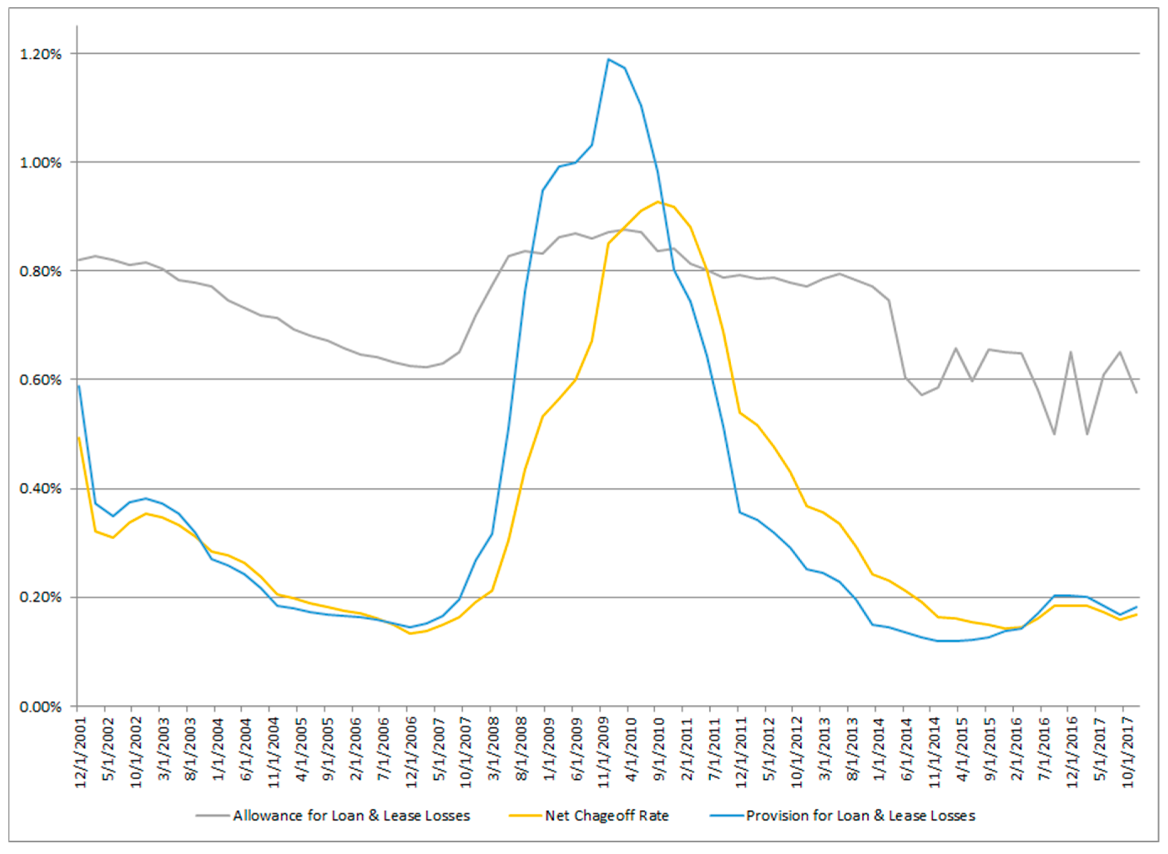
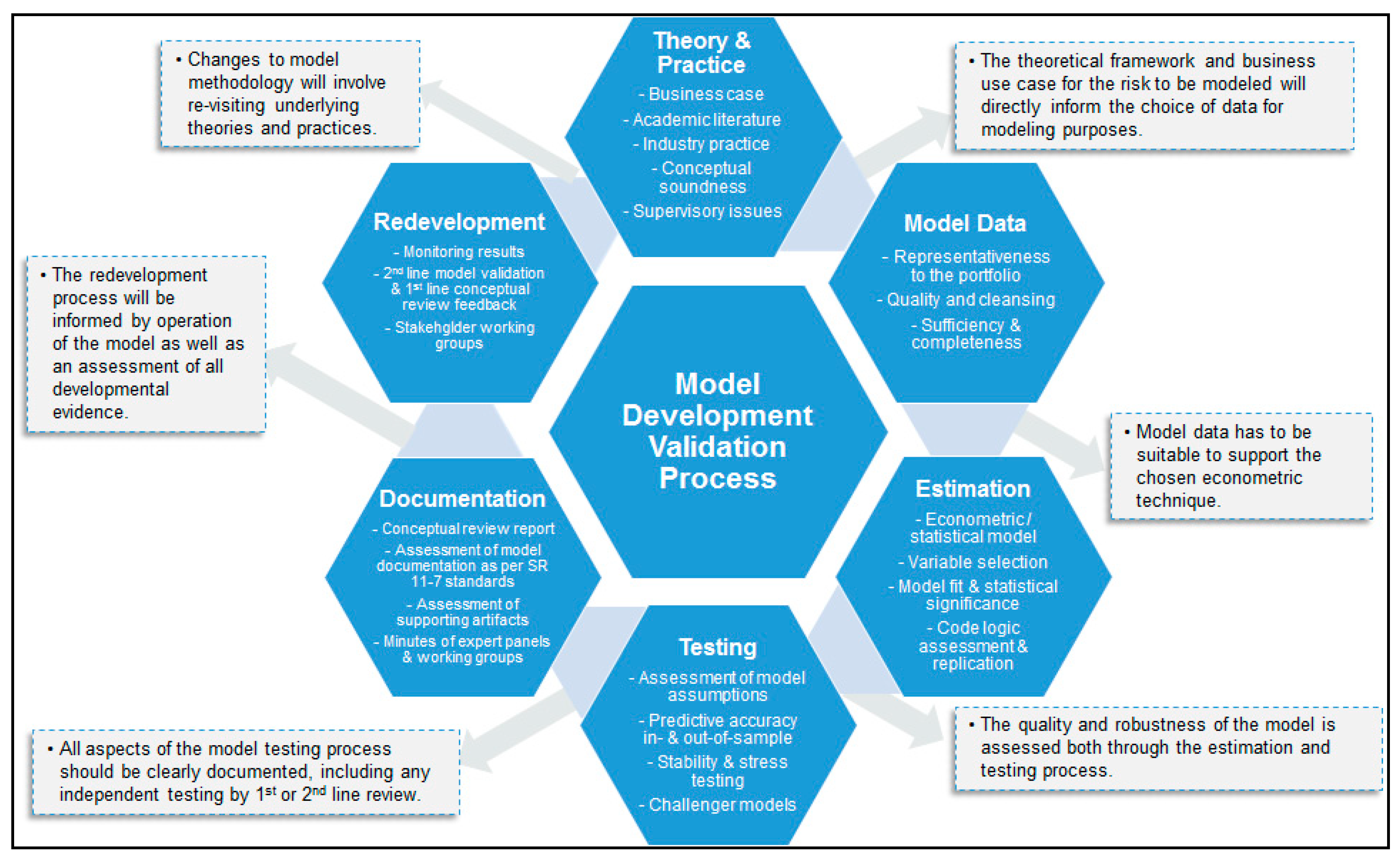
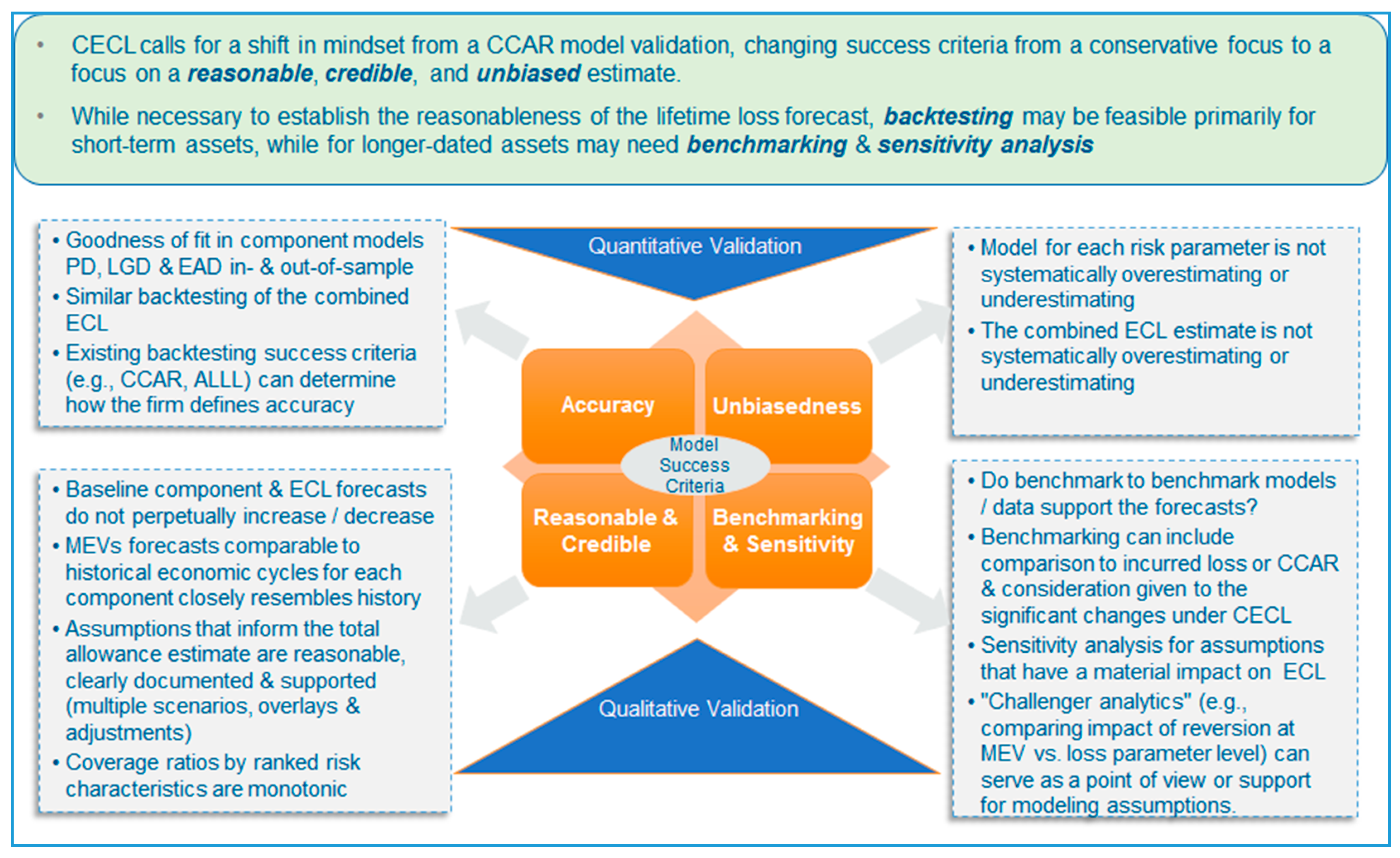
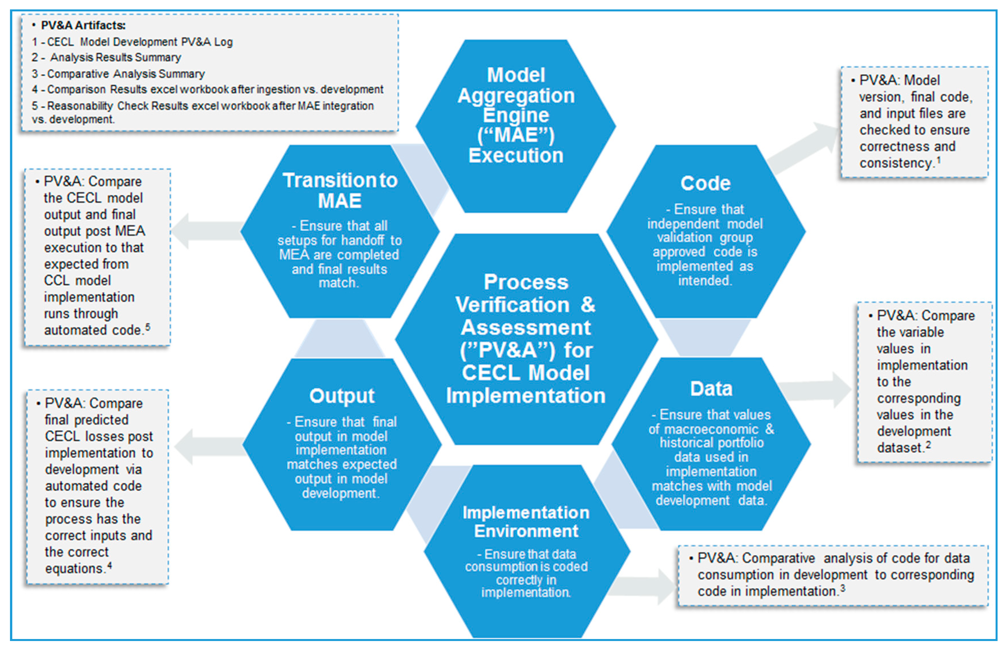
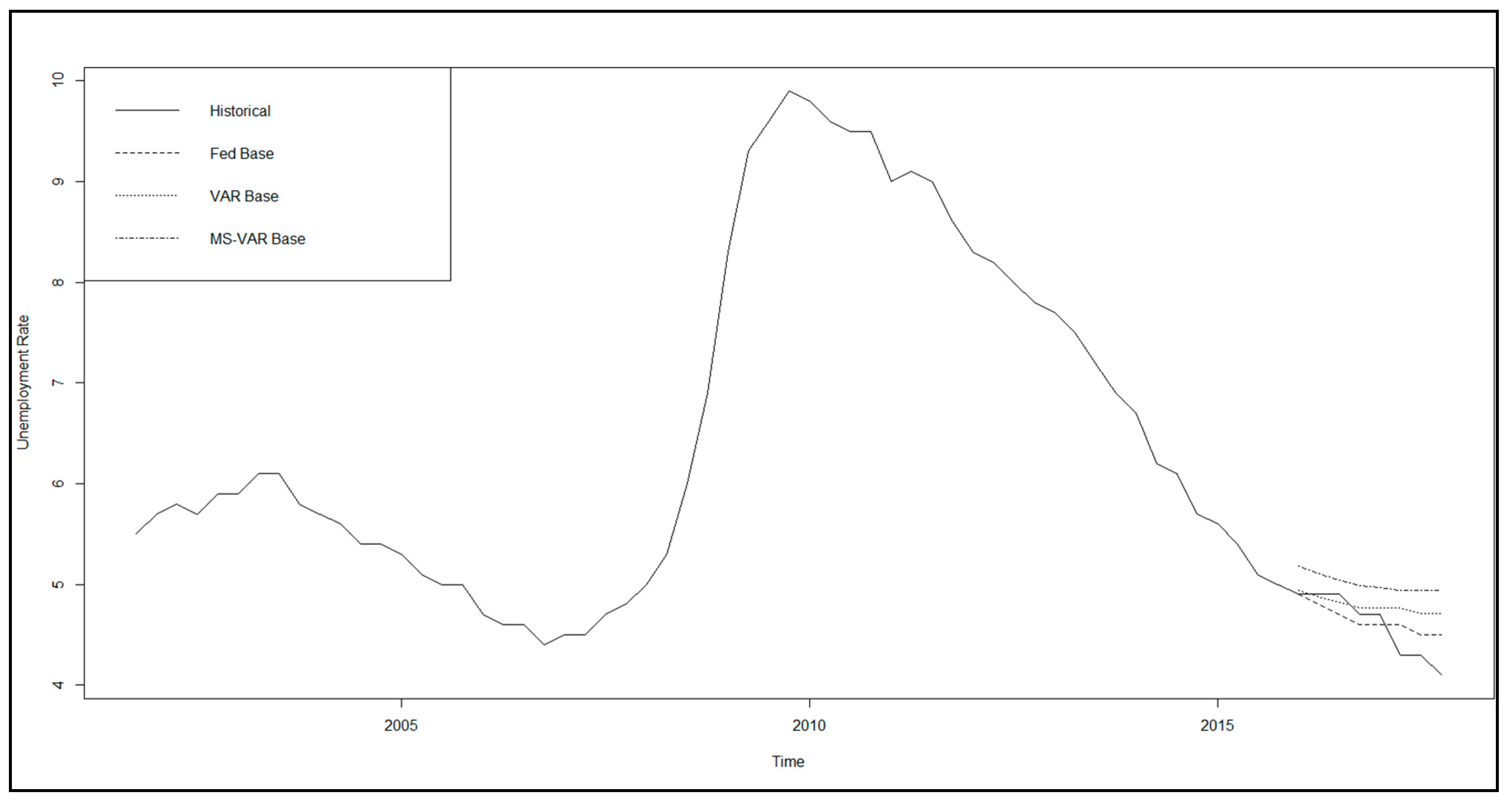
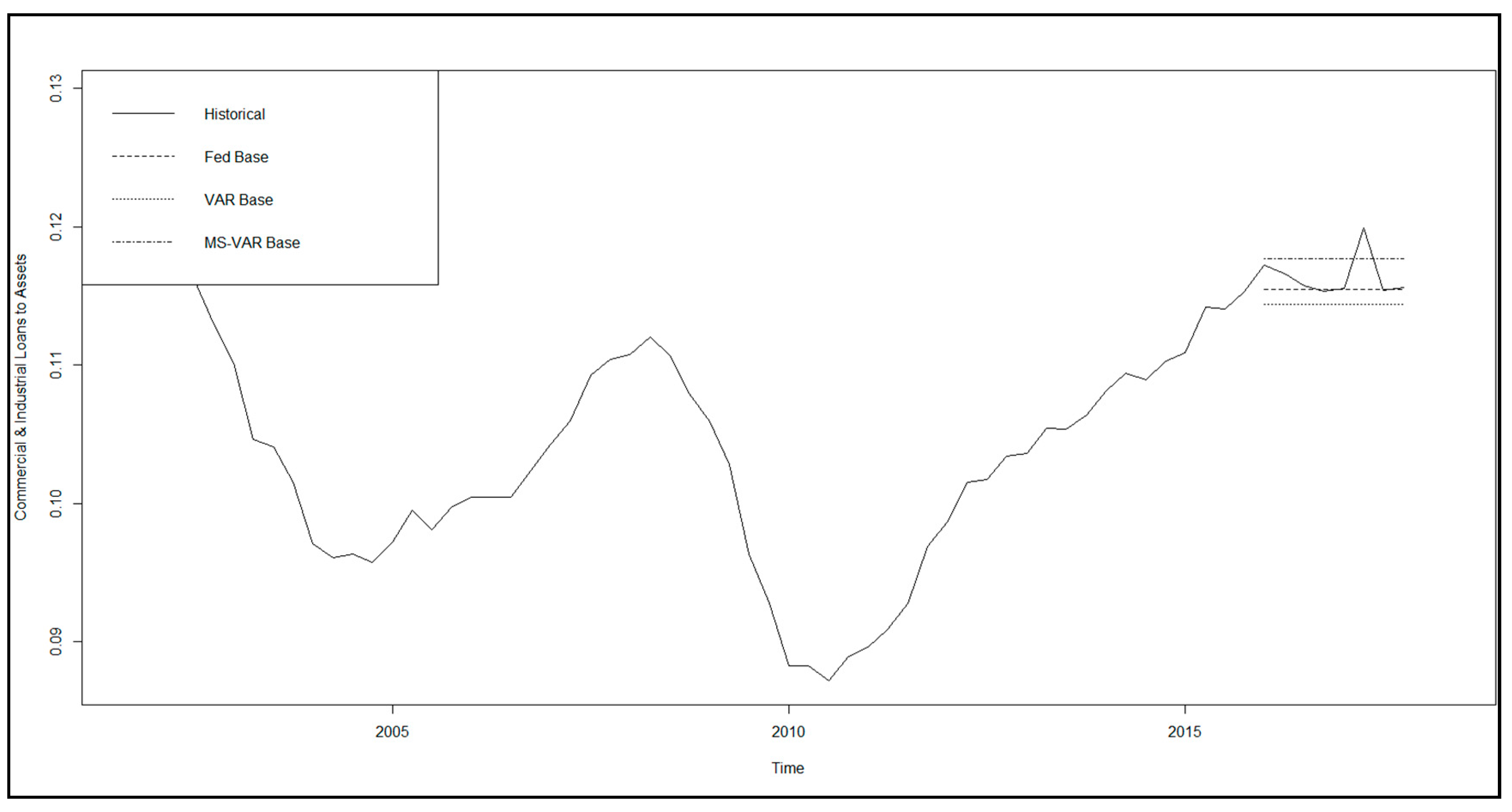
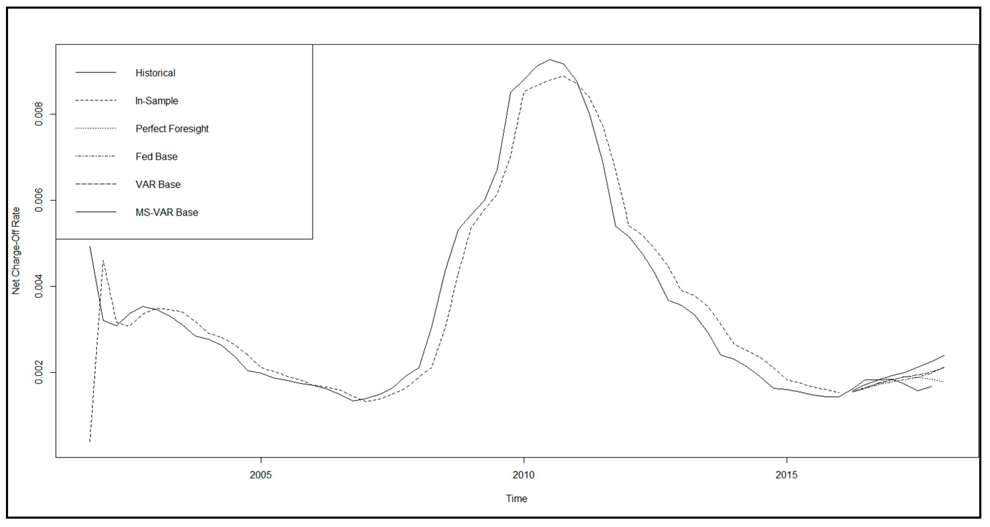
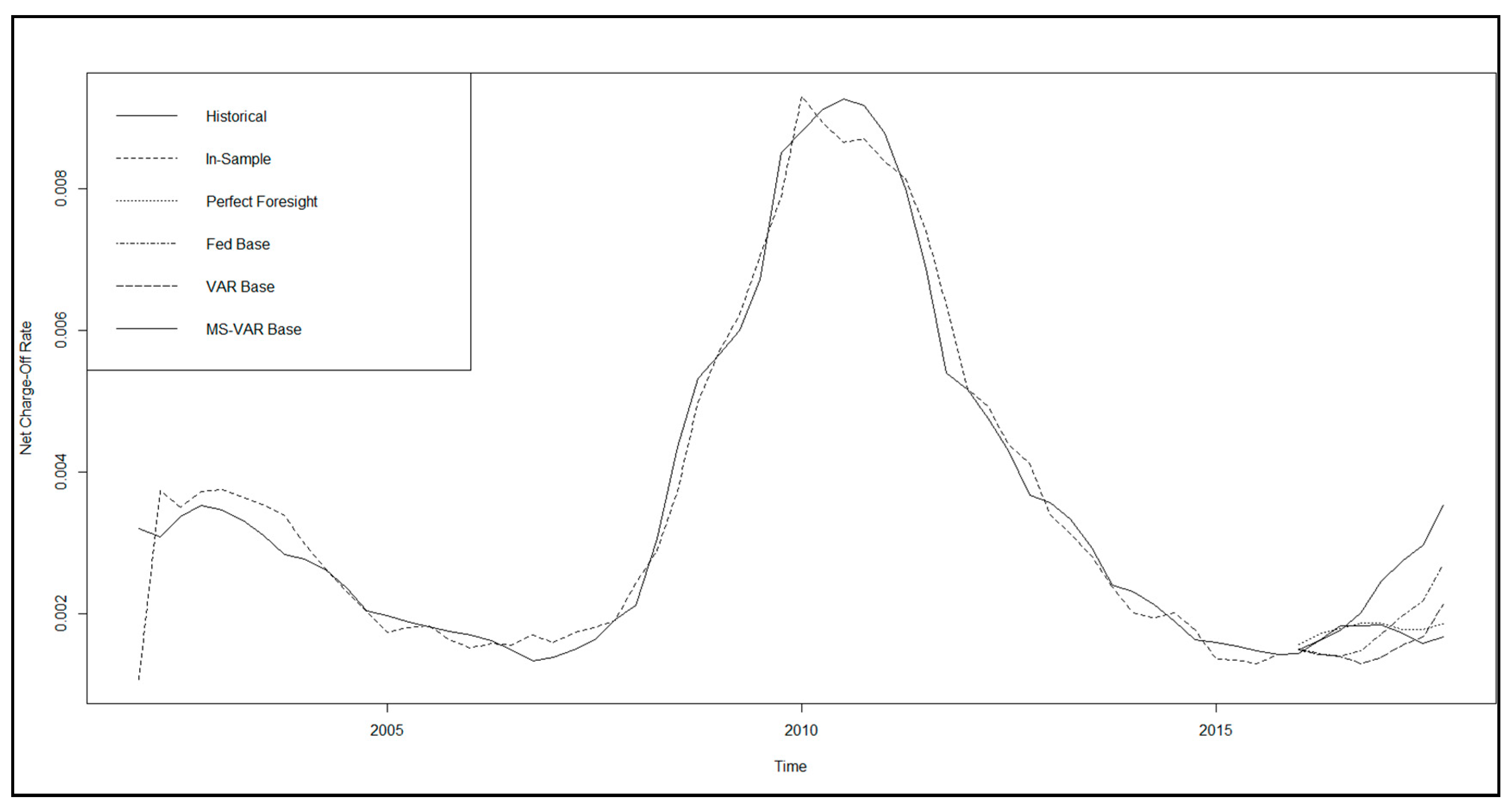
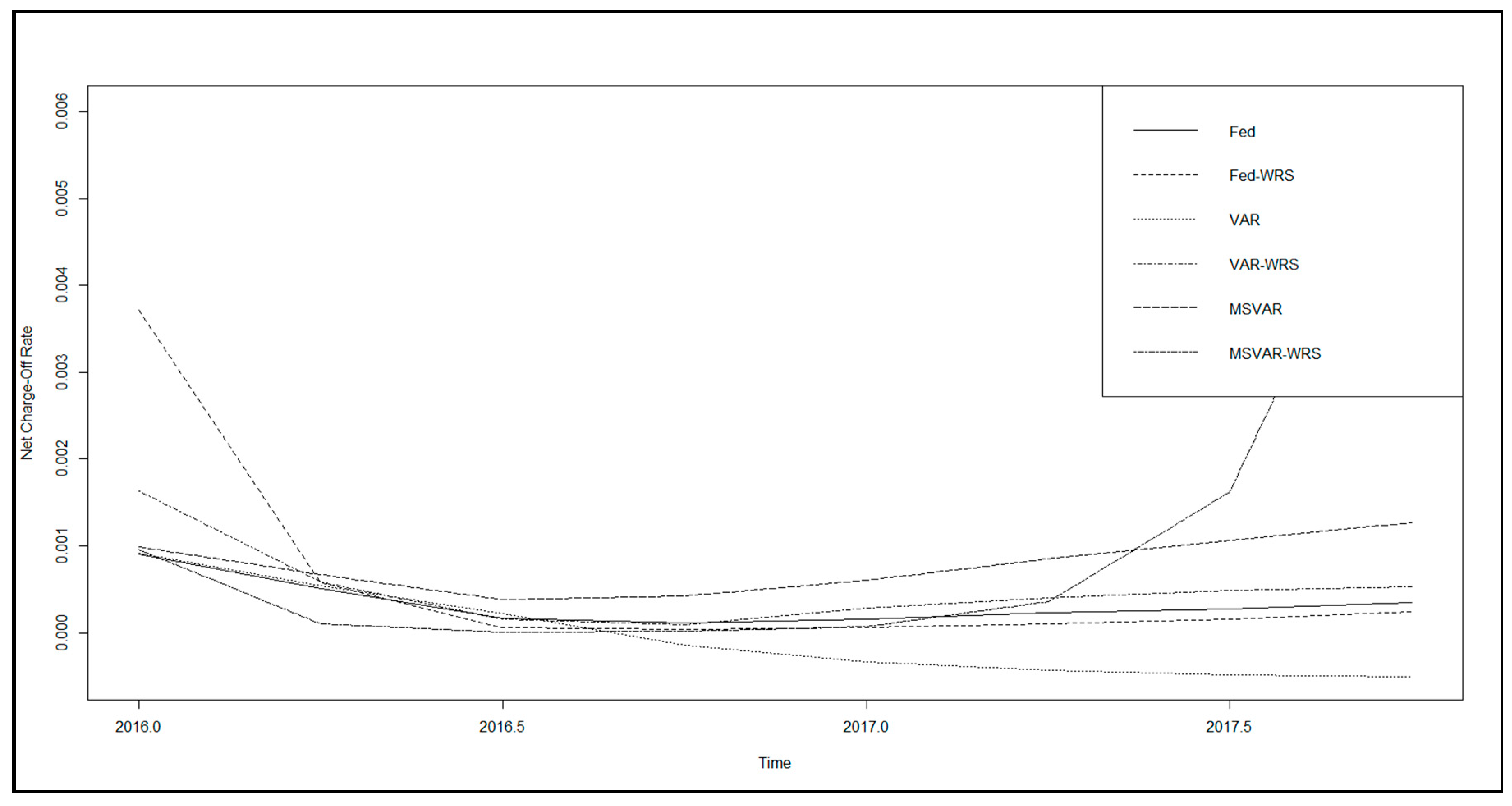
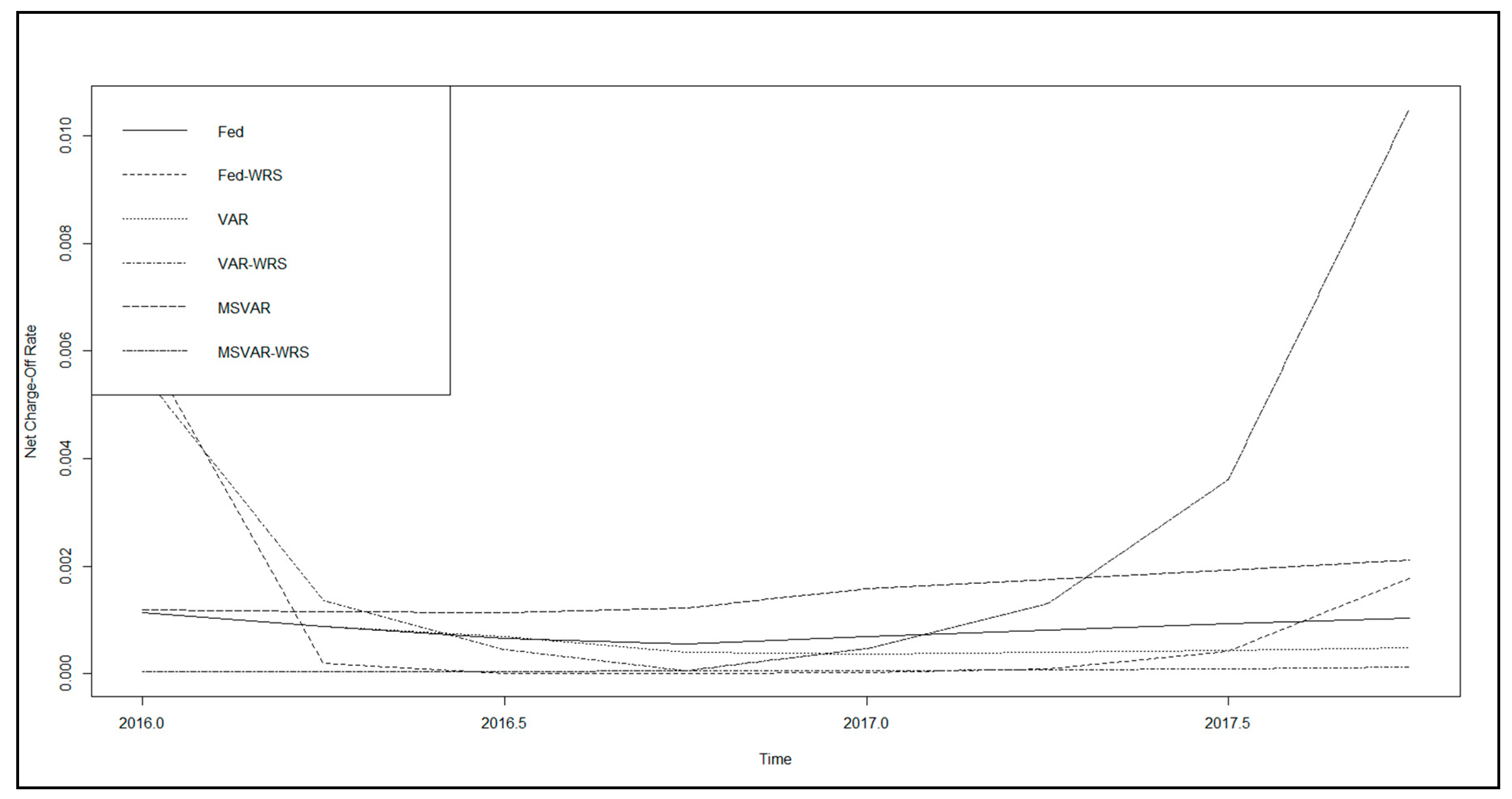
Table 1.
Summary statistics of historical Y9 credit loss rates, banking system idiosyncratic variables, and macroeconomic variables (FDIC SDI Report and Federal Reserve Board 4Q91–4Q15).
Table 1.
Summary statistics of historical Y9 credit loss rates, banking system idiosyncratic variables, and macroeconomic variables (FDIC SDI Report and Federal Reserve Board 4Q91–4Q15).
| Input Variables—Idiosyncratic Variables | Input Variables—Macroeconomic Variables | ||||||||||
|---|---|---|---|---|---|---|---|---|---|---|---|
| NCOR | CIL | CDL | TAA | OREO | TTUC | UNEMP | BBBCY | CREPI | VIX | CORPSPR | |
| Count | 65 | 65 | 64 | 65 | 65 | 64 | 65 | 65 | 65 | 65 | 65 |
| Mean | 0.35% | 0.10 | 0.01 | 0.05 | 0.001 | 0.01 | 6.31 | 5.54 | 201.12 | 26.56 | 2.99 |
| StdDev. | 0.23% | 0.01 | 0.05 | 0.01 | 0.0010 | 0.03 | 1.73 | 1.29 | 40.64 | 12.09 | 1.15 |
| Min. | 0.13% | 0.09 | −0.09 | 0.03 | 0.001 | −0.09 | 4.10 | 3.70 | 138.70 | 12.70 | 1.40 |
| 25 Prc. | 0.17% | 0.10 | −0.04 | 0.04 | 0.001 | −0.001 | 5.00 | 4.50 | 167.30 | 18.90 | 2.30 |
| Med. | 0.26% | 0.1054 | 0.02 | 0.06 | 0.0009 | 0.013 | 5.70 | 5.50 | 198.50 | 22.70 | 3.00 |
| 75 Prc. | 0.44% | 0.11 | 0.04 | 0.05 | 0.002 | 0.02 | 7.70 | 6.40 | 234.0 | 30.80 | 3.50 |
| Max. | 0.93% | 0.13 | 0.16 | 0.08 | 0.004 | 0.06 | 9.90 | 9.40 | 278.70 | 80.90 | 7.20 |
| CV | 0.67 | 0.09 | 7.21 | 0.20 | 0.73 | 4.53 | 0.27 | 0.23 | 0.20 | 0.46 | 0.38 |
| Skew | 1.32 | 0.1477 | −0.21 | 0.46 | 0.91 | −1.25 | 0.80 | 0.77 | 0.21 | 1.96 | 1.50 |
| Kurt. | 0.67 | −0.24 | −0.06 | 0.16 | −0.59 | 2.05 | −0.72 | 0.34 | −1.12 | 5.51 | 4.13 |
Table 2.
Correlations of historical Y9 credit loss rates, banking system idiosyncratic variables, and macroeconomic variables (FDIC SDI Report and Federal Reserve Board 4Q91–4Q15).
Table 2.
Correlations of historical Y9 credit loss rates, banking system idiosyncratic variables, and macroeconomic variables (FDIC SDI Report and Federal Reserve Board 4Q91–4Q15).
| NCOR | CIL | CDL | TAA | OREO | TTUC | UN-EMP | BBBCY | CREPI | VIX | CORP-SPR | |
|---|---|---|---|---|---|---|---|---|---|---|---|
| NCOR | |||||||||||
| CIL | −0.59 | ||||||||||
| CDL | −0.82 | 0.39 | |||||||||
| TAA | 0.63 | −0.43 | −0.34 | ||||||||
| OREO | 0.69 | −0.59 | −0.84 | 0.06 | |||||||
| TUC | −0.64 | 0.13 | 0.61 | −0.07 | −0.59 | ||||||
| UNEMP | 0.91 | −0.62 | −0.80 | 0.30 | 0.94 | −0.41 | |||||
| BBBCY | 0.52 | −0.25 | −0.31 | 0.48 | 0.13 | −0.17 | 0.07 | ||||
| CREPI | −0. 80 | 0.56 | 0.58 | −0.13 | −0.66 | 0.25 | −0.54 | −0.41 | |||
| VIX | 0.64 | −0.22 | −0.52 | 0.05 | 0.45 | −0.27 | 0.38 | 0.60 | −0.22 | ||
| CORPSPR | 0.69 | −0.45 | −0.55 | 0.08 | 0.45 | −0.21 | 0.61 | 0.47 | −0.25 | 0.81 |
Table 3.
Vector autoregressive CECL model estimation results compared—historical Y9 credit loss rates, banking system idiosyncratic, and macroeconomic variables (FDIC SDI Report and Federal Reserve Board 4Q91–4Q15).
Table 3.
Vector autoregressive CECL model estimation results compared—historical Y9 credit loss rates, banking system idiosyncratic, and macroeconomic variables (FDIC SDI Report and Federal Reserve Board 4Q91–4Q15).
| Statistics | NCOR Lag | Int. | UN-EMP | BBBCY | CREPI | BBBCY | VIX | CILTA | CD-LGR | TAATA | OREO-TA | TUCG |
|---|---|---|---|---|---|---|---|---|---|---|---|---|
| Esti. | −0.69 | −0.31% | 0.16% | 0.04% | ||||||||
| PV | 1.0 × 10⁻¹⁰ | 1.0 × 10⁻¹⁰ | 1.6 × 10⁻³ | 3.1 × 10⁻⁴ | ||||||||
| AR2 | 92.62% | |||||||||||
| Esti. | −0.67 | −0.04% | 0.01% | 0.03% | −0.9% | −0.78% | ||||||
| PV | 1.0 × 10⁻¹⁰ | 5.2 × 10⁻³ | 1.9 × 10⁻³ | 1.0 × 10⁻³ | 1.0 × 10⁻⁹ | 1.0 × 10⁻⁹ | ||||||
| AR2 | 96.69% | |||||||||||
| Esti. | −0.71 | −0.03% | 0.23% | 0.02% | ||||||||
| PV | 1.0 × 10⁻¹⁰ | 3.1 × 10⁻² | 2.0 × 10⁻³ | 1.6 × 10⁻² | ||||||||
| AR2 | 89.69% | |||||||||||
| Est. | −0.70 | −0.03% | 0.01% | −0.43% | −0.66% | 4.75% | ||||||
| PV | 1.0 × 10⁻¹⁰ | 6.2 × 10⁻² | 2.6 × 10⁻² | 2.0 × 10⁻¹³ | 1.6 × 10⁻⁷ | 1.0 × 10⁻¹⁰ | ||||||
| AR2 | 95.55% | |||||||||||
| Est. | −0.70 | −0.05% | 0.01% | 0.01% | ||||||||
| PV | 1.0 × 10⁻¹⁰ | 3.5 × 10⁻³ | 3.0 × 10⁻² | 2.8 × 10⁻³ | ||||||||
| AR2 | 87.45% | |||||||||||
| Est. | −0.85 | 0.01% | 0.05% | 0.01% | ||||||||
| PV | 1.0 × 10⁻¹⁰ | 2.8 × 10⁻² | 3.5 × 10⁻³ | 1.2 × 10⁻² | ||||||||
| AR2 | 94.88% | |||||||||||
| Est. | −0.82 | −0.12% | −0.20% | 0.06% | ||||||||
| PV | 1.0 × 10⁻¹⁰ | 1.1 × 10⁻¹¹ | 6.7 × 10⁻³ | 8.9 × 10⁻⁷ | ||||||||
| AR2 | 87.45% | |||||||||||
| Est. | −0.79 | −0.29% | −0.30% | 0.04% | 5.0% | 9.22% | ||||||
| PV | 1.0 × 10⁻¹⁰ | 1.0 × 10⁻¹⁰ | 4.2 × 10⁻⁷ | 2.5 × 10⁻⁴ | 1.0 × 10⁻¹⁰ | 3.5 × 10⁻³ | ||||||
| AR2 | 95.18% | |||||||||||
| Est. | −0.89 | 0.003% | 0.00% | 0.06% | ||||||||
| PV | 1.0 × 10⁻¹⁰ | 4.0 × 10⁻² | 4.9 × 10⁻³ | 2.3 × 10⁻⁷ | ||||||||
| AR2 | 92.82% | |||||||||||
| Est. | −0.88 | −0.18% | 0.001% | 0.01% | −0.61% | |||||||
| PV | 1.0 × 10⁻¹⁰ | 1.0 × 10⁻¹⁰ | 4.9 × 10⁻³ | 2.2 × 10⁻² | 2.3 × 10⁻² | |||||||
| AR2 | 92.88% | |||||||||||
| Est. | −0.79 | −0.13% | 0.01% | 0.02% | −0.22% | |||||||
| PV | 1.0 × 10⁻¹⁰ | 5.0 × 10⁻¹⁵ | 1.2 × 10⁻² | 1.5 × 10⁻² | 8.4 × 10⁻⁴ | |||||||
| AR2 | 91.97% | |||||||||||
| Est. | −0.85 | 0.03% | 0.01% | 0.02% | −0.25% | −0.54% | ||||||
| PV | 1.0 × 10⁻¹⁰ | 1.3 × 10⁻² | 1.5 × 10⁻³ | 4.6 × 10⁻² | 2.6 × 10⁻⁷ | 1.2 × 10⁻⁶ | ||||||
| AR2 | 96.44% | |||||||||||
| Est. | −0.65 | −0.35% | 0.05% | 0.04% | 0.02% | |||||||
| PV | 0 | 0 | 5.0 × 10⁻⁶ | 1.1 × 10⁻⁴ | 5.6 × 10⁻⁴ | |||||||
| AR2 | 93.12% | |||||||||||
| Esti. | −0.85 | −0.31% | 0.001% | 0.03% | 0.01% | 3.6% | ||||||
| PV | 1.0 × 10⁻¹⁰ | 1.0 × 10⁻¹⁰ | 4.6 × 10⁻⁴ | 7.9 × 10⁻³ | 2.8 × 10⁻² | 1.0 × 10⁻¹⁰ | ||||||
| AR2 | 94.71% | |||||||||||
Table 4.
CECL vector autoregressive model of in- and out-of-sample performance measures compared—historical Y9 credit loss rates, banking system idiosyncratic, and macroeconomic variables (FDIC SDI Report, Federal Reserve Board 4Q91–4Q15 and Jacobs (2018) models).
| Time Period | Statistic | Model | |||||||||||||
|---|---|---|---|---|---|---|---|---|---|---|---|---|---|---|---|
| UNEMP & CORP-SPR | UNEMP, CORP-SPR, TAATA & CDLG | UNEMP & CREPI | UNEMP, CREPI, TAATA & CDLG | UNEMP & CORP-SPR | UNEMP, CORP-SPR & OREOTA | CREPI & VIX | CREPI, VIX, OREOTA & TAATA | VIX, UNEMP & CORP-SPR | VIX, UNEMP, CORPSPR & TUCLG | BBBCY, UNEMP & CREPI | BBBCY, UNEMP, CREPI & CDLG | BBBCY, UNEMP & CORPSPR | BBBCY, UNEMP. CORPSPR & TAATA | ||
| Development Sample | GCV | 1.2 × 10⁻¹⁰ | 1.3 × 10⁻¹⁰ | 1.7 × 10⁻¹⁰ | 1.0 × 10⁻¹¹ | 2.0 × 10⁻¹⁰ | 1.0 × 10⁻¹⁰ | 1.0 × 10⁻¹⁰ | 1.0 × 10⁻¹¹ | 1.0 × 10⁻¹⁰ | 1.0 × 10⁻¹⁰ | 1.0 × 10⁻¹⁰ | 6.0 × 10⁻¹¹ | 1.1 × 10⁻¹⁰ | 1.1 × 10⁻¹⁰ |
| SC | 93.1% | 97.1% | 90.1% | 95.9% | 88.9% | 95.2% | 90.0% | 95.7% | 93.4% | 93.7% | 92.8% | 96.8% | 93.7% | 95.3% | |
| RMSE | 6.4 × 10⁻⁴ | 6.6 × 10⁻⁴ | 7.7 × 10⁻⁴ | 5.3 × 10⁻⁴ | 8.2 × 10⁻⁴ | 5.6 × 10⁻⁴ | 7.8 × 10⁻⁴ | 5.5 × 10⁻⁴ | 6.6 × 10⁻⁴ | 6.5 × 10⁻⁴ | 6.7 × 10⁻⁴ | 4.5 × 10⁻⁴ | 6.2 × 10⁻⁴ | 5.7 × 10⁻⁴ | |
| CPE | −0.02% | 0.02% | 0.02% | 0.01% | −0.01% | −0.10% | −0.01% | 0.09% | 0.10% | 0.14% | 0.04% | −0.02% | 0.21% | 0.04% | |
| AIC | −603.0 | −589.5 | −591.6 | −583.1 | −584.9 | −589.2 | −590.8 | −579.0 | −561.0 | −561.4 | −598.5 | −631.7 | −606.6 | −576.3 | |
| Perfect Forecast Prediction | GCV | 4.8 × 10⁻⁸ | 2.0 × 10⁻⁸ | 1.6 × 10⁻⁹ | 1.6 × 10⁻⁹ | 3.0 × 10⁻¹⁰ | 1.1 × 10⁻⁸ | 1.5 × 10⁻⁸ | 2.9 × 10⁻⁸ | 71.0 × 10⁻⁹ | 1.1 × 10⁻⁸ | 8.1 × 10⁻⁹ | 2.7 × 10⁻¹⁰ | 7.1 × 10⁻⁸ | 4.3 × 10⁻⁸ |
| SC | 0.40% | 3.8% | 5.2% | 7.9% | 50.4% | 0.10% | 10.1% | 42.1% | 30.3% | 19.7% | 1.2% | 68.4% | 2.1% | 6.6% | |
| RMSE | 0.0020 | 0.0020 | 0.0004 | 0.0010 | 0.0002 | 0.0010 | 0.0010 | 0.0020 | 0.0010 | 0.0020 | 0.0010 | 0.0002 | 0.0030 | 0.0030 | |
| CPE | −86.0% | −50.0% | 5.5% | −30.0% | 4.9% | −40.0% | 38.1% | −67.1% | 29.2% | 35.6% | −32.8% | 5.1% | −103.8% | −67.5% | |
| AIC | −79.0 | −82.3 | −106.5 | −89.0 | −119.0 | −88.5 | −88.6 | −79.2 | −92.5 | −86.8 | −91.3 | −116.5 | −74.0 | −76.0 | |
| Fed Base Prediction | GCV | 4.0 × 10⁻⁸ | 2.2 × 10⁻⁸ | 6.0 × 10⁻¹⁰ | 170 × 10−8 | 1.1 × 10⁻⁹ | 2.6 × 10⁻⁸ | 6.5 × 10⁻³ | 1.9 × 10⁻⁷ | 7.8 × 10⁻⁸ | 1.3 × 10⁻⁷ | 1.8 × 10⁻⁸ | 4.7 × 10⁻⁹ | 2.0 × 10⁻⁸ | 9.1 × 10⁻⁸ |
| SC | 80.2% | 87.3% | 21.8% | 29.0% | 4.9% | 4.5% | 0.7% | 0.2% | 0.8% | 0.44% | 81.8% | 2.0% | 1.4% | 9.7% | |
| RMSE | 0.0020 | 0.0020 | 0.0002 | 0.0020 | 0.0003 | 0.0010 | 0.0020 | 0.0100 | 0.0030 | 0.0050 | 0.0020 | 0.0010 | 0.0020 | 0.0040 | |
| CPE | −80.1% | −58.9% | −7.4% | −49.0% | 7.4% | −61.0% | −715.0% | −152.0 | −80.0% | −100.6% | −50.6% | 6.1% | 48.9% | −35.4% | |
| AIC | −80.5 | −81.2 | −113.9 | −83.2 | −109.2 | −82.0 | −77.8 | −64.3 | −73.2 | −67.2 | −85.4 | −93.7 | −83.9 | −70.0 | |
| VAR Model Base Prediction | GCV | 6.7 × 10⁻⁸ | 4.2 × 10⁻⁸ | 4.7 × 10⁻¹⁰ | 1.7 × 10⁻⁸ | 1.2 × 10⁻⁹ | 1.1 × 10⁻⁸ | 6.3 × 10⁻⁸ | 2.1 × 10⁻⁷ | 8.6 × 10⁻⁸ | 1.4 × 10⁻⁷ | 2.7 × 10⁻⁸ | 2.5 × 10⁻⁹ | 4.6 × 10⁻⁹ | 1.3 × 10⁻⁷ |
| SC | 23.7% | 27.8% | 13.8% | 28.7% | 9.58% | 4.9% | 0.60% | 0.10% | 0.74% | 0.34% | 45.7% | 9.9% | 12.5% | 7.3% | |
| RMSE | 0.0030 | 0.0030 | 0.0002 | 0.0020 | 0.0003 | 0.0010 | 0.0300 | 0.0100 | 0.0030 | 0.0050 | 0.0020 | 0.0010 | 0.0010 | 0.005 | |
| CPE | −102.0% | −80.2% | −2.6% | −47.2% | 9.0% | −40.4% | −75.0% | −158.0% | −83.4% | −104.8% | −64.7% | −8.7% | 25.8% | −59.0% | |
| AIC | −76.4 | −76.1 | −116.1 | −83.4 | −108.7 | −88.5 | −76.9 | −63.4 | −72.4 | −66.6 | −81.6 | −98.8 | −95.9 | −66.8 | |
| MS-VAR Model Base Prediction | GCV | 2.0 × 10⁻⁸ | 1.5 × 10⁻⁸ | 320 × 10−9 | 1.2 × 10⁻⁸ | 3.1 × 10⁻⁹ | 6.3 × 10⁻⁹ | 4.6 × 10⁻⁸ | 1.4 × 10⁻⁷ | 8.1 × 10⁻⁸ | 1.4 × 10⁻⁷ | 3.9 × 10⁻⁹ | 1.8 × 10⁻⁸ | 3.4 × 10⁻⁸ | 7.6 × 10⁻⁸ |
| SC | 46.2% | 42.97% | 0.63% | 7.71% | 4.62% | 0.40% | 0.30% | 2.1% | 0.80% | 0.44% | 0.42% | 1.1% | 85.1% | 12.3% | |
| RMSE | 0.0010 | 0.0020 | 0.0010 | 0.0020 | 0.0010 | 0.001 | 0.0020 | 0.0100 | 0.00300 | 0.0050 | 0.0010 | 0.0020 | 0.0020 | 0.0040 | |
| CPE | −53.9% | −45.6% | 13.0% | −19.0% | 16.9% | −30.5% | −65.0% | −136.0% | −80.3% | −105.9% | −10.6% | 37.4% | −73.8% | −26.9% | |
| AIC | −86.0 | −84.37 | −100.6 | −86.4 | −101.0 | −93.3 | −79.3 | −66.5 | −72.9 | −66.4 | −97.2 | −85.1 | −79.7 | −73.4 | |
Table 5.
Kullback–Leibler relative entropy worst-case loss for model risk quantification measures—vector autoregressive CECL out-of-sample models compared (FDIC SDI Report, Federal Reserve Board 4Q91–4Q15, and Jacobs (2018) models).
| Macroeconomic | Idiosyncratic | Fed | VAR | MS-VAR | Min | Avg | Stdev | Max | |
|---|---|---|---|---|---|---|---|---|---|
| UNEMP & BBBCY | None | Base | 0.0338% | 0.0448% | 0.0781% | 23.82% | 26.82% | 3.6% | 30.5% |
| Worse | 0.0617% | 0.0519% | 0.1146% | ||||||
| RMRE | 30.49% | 26.14% | 23.82% | ||||||
| UNEMP & BBBCY | CILA & CDLG | Base | 0.0696% | 0.0344% | 0.0920% | 25.61% | 30.17% | 5.6% | 36.5% |
| Worse | 0.0956% | 0.0713% | 0.1237% | ||||||
| RMRE | 36.47% | 28.43% | 25.61% | ||||||
| UNEMP & CREPI | None | Base | 0.1567% | 0.1648% | 0.1913% | 19.87% | 24.65% | 4.2% | 27.7% |
| Worse | 0.1642% | 0.1777% | 0.2300% | ||||||
| RMRE | 26.20% | 27.88% | 19.87% | ||||||
| UNEMP & CREPI | TAATA & CDLG | Base | 0.0868% | 0.0895% | 0.1366% | 25.15% | 31.25% | 5.3% | 34.7% |
| Worse | 0.1296% | 0.1364% | 0.2115% | ||||||
| RMRE | 33.92% | 34.69% | 25.15% | ||||||
| UNEMP & CORPSPR | None | Base | 0.1817% | 0.1845% | 0.1979% | 15.36% | 21.64% | 5.6% | 25.9% |
| Worse | 0.2059% | 0.2063% | 0.2289% | ||||||
| RMRE | 25.98% | 23.57% | 15.36% | ||||||
| UNEMP & CORPSPR | OREOTA | Base | 0.0661% | 0.1008% | 0.1177% | 21.58% | 26.11% | 3.9% | 28.6% |
| Worse | 0.1085% | 0.1305% | 0.1329% | ||||||
| RMRE | 28.14% | 28.62% | 21.58% | ||||||
| CREPI & VIX | None | Base | 0.1129% | 0.1166% | 0.1021% | 17.22% | 25.18% | 6.9% | 29.4% |
| Worse | 0.1711% | 0.1700% | 0.1614% | ||||||
| RMRE | 29.39% | 28.93% | 17.22% | ||||||
| CREPI & VIX | OREOTA & TAATA | Base | 0.1458% | 0.1564% | 0.1187% | 30.92% | 39.35% | 7.4% | 44.6% |
| Worse | 0.1026% | 0.1101% | 0.0714% | ||||||
| RMRE | 42.60% | 44.53% | 30.92% | ||||||
| VIX, UNEMP & CORPSPR | None | Base | 0.1331% | 0.1381% | 0.1361% | 29.65% | 36.78% | 6.3% | 41.7% |
| Worse | 0.1398% | 0.1436% | 0.1221% | ||||||
| RMRE | 39.00% | 41.69% | 29.65% | ||||||
| VIX, UNEMP & CORPSPR | TUCLG | Base | 0.1658% | 0.1718% | 0.1741% | 36.39% | 43.61% | 6.5% | 49.0% |
| Worse | 0.2162% | 0.2157% | 0.2091% | ||||||
| RMRE | 48.98% | 45.47% | 36.39% | ||||||
| BBBCY, UNEMP & CCREP | None | Base | 0.0836% | 0.0598% | 0.1513% | 33.63% | 39.64% | 5.2% | 42.7% |
| Worse | 0.1089% | 0.0972% | 0.2006% | ||||||
| RMRE | 42.70% | 42.57% | 33.63% | ||||||
| BBBCY, UNEMP & CCREP | CDLG | Base | 0.1796% | 0.1545% | 0.2326% | 41.44% | 47.41% | 5.4% | 51.9% |
| Worse | 0.2527% | 0.1990% | 0.3305% | ||||||
| RMRE | 51.91% | 48.89% | 41.44% | ||||||
| BBBCY, UNEMP & CORPSPR | None | Base | 0.2520% | 0.2128% | 0.0444% | 26.26% | 36.68% | 9.0% | 42.4% |
| Worse | 0.3330% | 0.2400% | 0.0723% | ||||||
| RMRE | 42.36% | 41.42% | 26.26% | ||||||
| BBBCY, UNEMP & CORPSPR | TAATA | Base | 0.1766% | 0.1981% | 0.1746% | 42.93% | 46.81% | 3.6% | 50.0% |
| Worse | 0.3231% | 0.3283% | 0.3194% | ||||||
| RMRE | 47.49% | 50.02% | 42.93% | ||||||
| Relative Model Risk Error Summary Statistics—Macroeconomic Scenario Generation Models | Min | 25.98% | 23.57% | 15.36% | |||||
| Avg | 37.54% | 36.63% | 27.84% | ||||||
| StdDev | 8.75% | 9.22% | 8.48% | ||||||
| Max | 51.91% | 50.02% | 42.93% | ||||||
| Relative Model Risk Error Summary Statistics—Total Macroeconomic Scenario Generation & Credit Loss Models | Min | 15.36% | |||||||
| Avg | 34.01% | ||||||||
| StdDev | 9.68% | ||||||||
| Max | 51.91% | ||||||||
© 2020 by the author. Licensee MDPI, Basel, Switzerland. This article is an open access article distributed under the terms and conditions of the Creative Commons Attribution (CC BY) license (http://creativecommons.org/licenses/by/4.0/).
Share and Cite
MDPI and ACS Style
Jacobs, M., Jr. A Holistic Model Validation Framework for Current Expected Credit Loss (CECL) Model Development and Implementation. Int. J. Financial Stud. 2020, 8, 27. https://0-doi-org.brum.beds.ac.uk/10.3390/ijfs8020027
AMA Style
Jacobs M Jr. A Holistic Model Validation Framework for Current Expected Credit Loss (CECL) Model Development and Implementation. International Journal of Financial Studies. 2020; 8(2):27. https://0-doi-org.brum.beds.ac.uk/10.3390/ijfs8020027
Chicago/Turabian StyleJacobs, Michael, Jr. 2020. "A Holistic Model Validation Framework for Current Expected Credit Loss (CECL) Model Development and Implementation" International Journal of Financial Studies 8, no. 2: 27. https://0-doi-org.brum.beds.ac.uk/10.3390/ijfs8020027
Note that from the first issue of 2016, this journal uses article numbers instead of page numbers. See further details here.