Article

Evidence of Intraday Multifractality in European Stock Markets during the Recent Coronavirus (COVID-19) Outbreak

1
Department of Management Sciences, COMSATS University, Islamabad 45550, Pakistan
2
Business School, Hanyang University, Seoul 04763, Korea
3
Department of Business Administration, Iqra University, Islamabad 75500, Pakistan
4
Department of Management, University of Évora, 7000 Évora, Portugal
5
VALORIZA—Research Center for Endogenous Resource Valorization, 7300-555 Portalegre, Portugal
6
Department of Economic Sciences and Organizations, Polytechnic Institute of Portalegre, 7300-555 Portalegre, Portugal
7
CEFAGE-UE, IIFA, University of Évora, 7000 Évora, Portugal
*
Author to whom correspondence should be addressed.
Int. J. Financial Stud. 2020, 8(2), 31; https://0-doi-org.brum.beds.ac.uk/10.3390/ijfs8020031
Submission received: 31 March 2020 / Revised: 20 May 2020 / Accepted: 25 May 2020 / Published: 26 May 2020
(This article belongs to the Special Issue Econophysics Applications to Financial Markets)

Abstract

:
This study assesses how the coronavirus pandemic (COVID-19) affects the intraday multifractal properties of eight European stock markets by using five-minute index data ranging from 1 January 2020 to 23 March 2020. The Hurst exponents are calculated by applying multifractal detrended fluctuation analysis (MFDFA). Overall, the results confirm the existence of multifractality in European stock markets during the COVID-19 outbreak. Furthermore, based on multifractal properties, efficiency varies among these markets. The Spanish stock market remains most efficient while the least efficient is that of Austria. Belgium, Italy and Germany remain somewhere in the middle. This far-reaching outbreak demands a comprehensive response from policy makers to improve market efficiency during such epidemics.
JEL Classification:
C10; G15

1. Introduction

This study assesses intraday multifractality in European stock markets by applying a robust physics-based statistical method. Our findings contribute to the financial literature by focusing on the behavior of the stock markets in question at the time of the coronavirus pandemic (COVID-19).
According to the World Health Organization (WHO), COVID-19 had led to more than 520,360 confirmed infected cases and 23,593 deaths in 198 countries by 27 March 2020. Besides the immediate tragedies of death and disease, indirect effects through fear are being felt around the world. The fear associated with the number of deaths reported has caused a sense of emergency and panic is spreading faster than the spread of the virus itself. According to International Labour Organization estimates, nearly 25 million jobs could be lost globally due to COVID-19 (for further details, see https://www.ilo.org/global/about-the-ilo/newsroom/news/WCMS_738742/lang--en/index.htm). Stock markets are characterized as sensitive and complex and can be manipulated by both internal and external factors. Investors and exchange institutions can be understood as internal factors, while the sources of external factors are reforms and announcements by governments or some important events. For investors, both local and global risk factors are significant. Variations in risk factors are likely to have a different effect on each country’s stock market performance.
Global stock markets are adjusting to the rapid emergence of COVID-19. For instance, on 16 March 2020 the Dow Jones Industrial Average dropped by 12.9% and the S&P 500 index lost nearly 12% in a single day. It was the worst percentage drop since the infamous “Black Monday” crash of 1987 (https://www.washingtonpost.com/business/2020/03/16/stocks-markets-today-coronavirus/). In the last month, UK-FTSE fell by 29.72%, Germany’s DAX by 33.37%, France’s CAC by 33.63%, Japan’s NIKKEI by 26.85% and the Indian SUNSEX by 17.74%.
The existing mainstream literature on financial markets is mainly based on the fundamental assumption of normal distribution of stock prices and the “random-walk” hypothesis (RWH) of Bachelier (1900). However, the econophysics literature rejects the RWH hypothesis and suggests that asset prices have different fundamental properties (Mandelbrot 1967, 1971, 1997), including fat tail (Gopikrishnan et al. 2001), long-term correlation (Alvarez-Ramirez et al. 2008), volatility clustering (Kim and Eom 2008), fractals and multifractals (He et al. 2007) and chaos (Adrangi et al. 2001). Since then, fractal analysis has been widely applied in financial market research. Using R/S analysis, Peters (1991, 1994) proved mono-fractal properties in several financial markets. However, mono-fractals cannot describe the height-height correlation function (Barabási and Vicsek 1991), Multifractal Detrended Fluctuation Analysis (MFDFA) (Kantelhardt et al. 2002; Alvarez-Ramirez et al. 2008) and the partition function method (Telesca et al. 2005; Kumar and Deo 2009; Yuan et al. 2009) Later, this method was applied in several fields with data structures, including finance (Podobnik and Stanley 2008; Wang et al. 2010; Mandelbrot et al. 1997; Kumar and Deo 2009; Oh et al. 2010).
Several studies focus particularly on market efficiency by applying econophysics methods. Various researchers use long-range dependence as a proxy of market inefficiency (Cajueiro and Tabak 2004; Christodoulou-Volos and Siokis 2006). In econophysics, one of the most popular methods of examining long-range dependence is the Detrended Fluctuation Analysis (DFA) proposed by (Peng et al. 1994). One of its major advantages lies in avoiding the spurious detection of long-range dependence in non-stationary data. For instance, Alvarez-Ramirez et al. (2008) used it to analyze crude oil markets and concluded on time-varying short-term inefficiency which became efficient in the long-run. Using the same method to explore Thai stock markets, Sukpitak and Hengpunya (2016) concluded that the most efficient market is the Stock Exchange of Thailand (SET), while the least efficient is the Market of Alternative Investment (MAI). This study also supported the assumption that market capitalization significantly affects market efficiency. In another study, Mohti et al. (2019) used both DFA and Mutual Information (MI) to investigate the long-range dependence in frontier markets. The study found weak-form efficiency only in the Slovenian market and concluded that other frontier markets located in Europe and America are less inefficient, while the least efficient markets are located in the Middle East.
As a generalization of DFA, Kantelhardt et al. (2002) introduced the MFDFA, applied to explore multifractality in time series data. Very recently, Miloş et al. (2020) employed MFDFA on daily data to investigate the efficiency of Central and Eastern European (CEE) stock markets such as Poland, the Czech Republic, Romania, Croatia, Hungary, Bulgaria and Slovenia. Their findings confirmed a lower degree of market efficiency. Similarly, Ferreira (2018) studied 18 Eastern European stock markets and showed that the majority of stock markets are far from being without long-range dependence, which could be seen as inefficiency. The results also showed that a few stock markets such as Hungary, the Czech Republic and Poland have decreasing dependence over time. Likewise, Norouzzadeh and Rahmani (2006) used this method to prove that the exchange market is also not efficient.
Considering the crisis period, Caraiani (2012) explored Central and Eastern Europe stock markets, finding multifractality during the global financial crisis. In addition, the study found no direct link between the crisis and the multifractal spectrum. Horta et al. (2014) also studied the impact of the 2008 and 2010 crises on the stock markets of Belgium, France, Greece, Japan, the Netherlands, Portugal, the UK and the US. The study used a combination of MFDMA and copula models. The findings from the former method suggested that most of the returns showed a long memory during 2008 crisis period, but this is not the case in either the pre-crisis period or during the 2010-crisis period. From a different perspective, Rizvi et al. (2014) also employed MFDFA to compare Islamic and developed markets and confirmed that Islamic countries had highly efficient performance in the crisis.
Most studies use daily data to analyze efficiency when using MFDFA methods. However, several studies also used high frequency data (Shahzad et al. 2018; Ruan and Zhou 2011). The study by Shahzad et al. (2018) confirmed the higher level of efficiency in the Japanese Yen (JPY) and the Swiss Franc (CHF) for both full and rolling window analysis. The results also indicated that the British Pound (GBP) is the least efficient exchange rate, followed by the Euro (EUR). With respect to stock markets, Ruan and Zhou (2011) used 1-min intertrade duration time series and confirmed the presence of intertrade durations of a multifractal nature in Chinese firms.
This study is different from previous ones and makes three contributions to the financial literature. Firstly, we use five-minute high frequency data of major European stock markets (Italy, France, Germany, Spain, Austria, Belgium, the United Kingdom and the Netherlands), since the COVID-19 pandemic is now focused on Europe. Secondly, we use Seasonal and Trend Decomposition using Loess (STL) to decompose intraday stock market returns. Thirdly, this study uses one of the most popular robust, physics-based techniques, the MFDFA as a generalization of DFA, as proposed by Kantelhardt et al. (2002), to detect the multifractal behavior of European stock markets during the COVID-19 outbreak. The MFDFA allows the estimation of multiple scaling exponents within the time series. Moreover, MFDFA is a renowned technique, but is not widely applied to high frequency data. Therefore, there is still room for in-depth analysis to understand the intraday behavior of European stock markets during the COVID-19 pandemic. The results show that the richest level of multifractality is found in the Austrian and UK stock markets and the lowest degree of dependence is evident in the Spanish stock market when COVID-19 was at its peak. The findings of this study will help regulators to protect stock markets by revealing the impacts of COVID-19 on European stock markets.
The remainder of the study is organized as follows: Section 2 describes the data and the methodology, followed by the empirical results and conclusions.

2. Materials and Methods

2.1. Data Description

The intraday stock index price per minute data was collected from DataStream from 1 January 2020 to 23 March 2020. However, due to countries’ lockdown and shutdown, most countries have a significant amount of per minute data missing. To overcome duplicate values, we aggregated the per minute data into a five-minute frequency. At a second stage, we deleted a few missing values at five-minute frequency. Finally, we were left with 8 European stock markets, namely Italy, France, Germany, Spain, Belgium, Austria, the Netherlands and the United Kingdom. Using five-minute frequency, we have 102 observations per day for 58 days which makes a total of 5916 observations. The list of countries, stock market indexes and number of observations are presented in Table 1.

2.2. Methodology

The analysis of five-minute stock market returns is divided into three stages.

2.2.1. Stage 1

To Begin With, The Five-Minute Log Return Is Defined as
r i   ( t ) = l n p i ( t ) l n p i ( t Δ t )
where the closing price of the index i is represented by p i ( t ) and the time interval is Δ t .
Figure 1 shows five-minute fluctuations in the Italian stock market index (FTMIB) from 1 January 2020 to 23 March 2020. It is clear that the market was stable until the third week of Feb-2020. After that there is a sudden decline in the market. This is significant to note the timelines of stock markets and the COVID-19 outbreak in Europe. According to the daily UN report, there were only 3 confirmed cases in Italy on 21 February 2020. A week later, there were 888 confirmed cases on 28 February 2020. By 21 March 2020 there were 53,578 confirmed cases in Italy, 25,734 in Spain, 22,213 in France and 14,282 in Germany. The other seven European stock markets show the same patterns and are attached in Supplementary files.

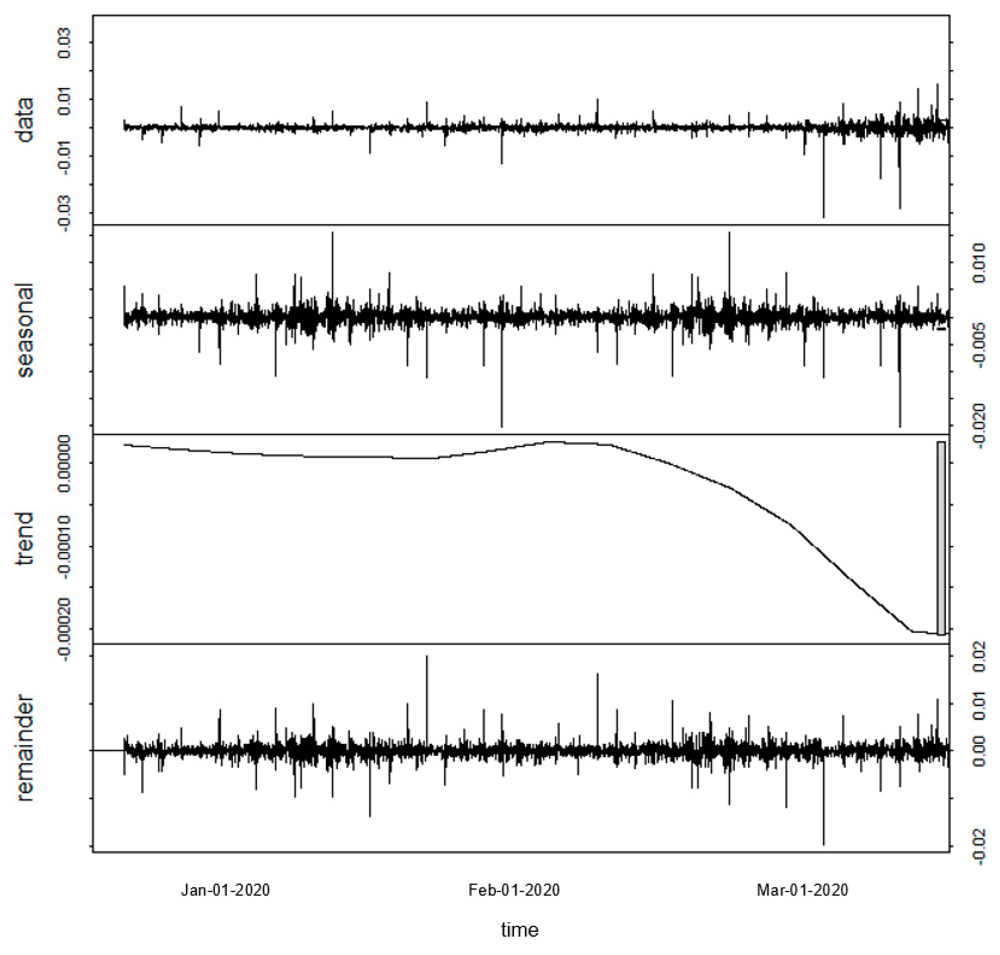
2.2.2. Stage 2: Seasonal and Trend Decomposition using Loess (STL)

Prior to MFDFA, we employed the Seasonal and Trend Decomposition using Loess (STL) method to decompose time series, as proposed by (Cleveland et al. 1990), which estimates nonlinear relationships. As we are using five-minute returns, STL is a versatile, robust method to handle any type of seasonality. Furthermore, this method is robust to outliers and flexible enough to allow seasonal component variations over time. In addition to improved reliability and decomposition by removing the seasonal components, the STL method also reveals inner dynamics of asset returns (Laib et al. 2018a, 2018b).
STL divides a time series into the trend, seasonality and remainder. In this study, we first decomposed the five-minute returns series into deterministic and stochastic components based on the Loess smoother, proposed by (Cleveland et al. 1990). The STL method breaks each stock return time series into a deterministic trend (Ti), seasonal (Si) components, and stochastic remainder (Ri) component, according to Laib et al. (2018a, 2018b) and Miloş et al. (2020), i.e.,:
r i   ( t ) = T i + S i + R i
For decomposition, we used the R package to employ STL decomposition (Laib et al. 2018a; Shiskin 1965; Miloş et al. 2020) (the details of STL are available at https://www.rdocumentation.org/packages/stats/versions/3.6.2/topics/stl). In our five-minute frequency, we set the span of the Loess window for seasonal extraction equal to 102, which is the number of trading prices in one day.
Figure 2 shows the STL decomposition of Italian stock index (FTMIB) returns. The four graphs correspond to the original five-minute returns data, seasonal component, trend component and the remainder. Similar results of STL decomposition of intraday index returns for the other seven stock indexes are available in the Supplementary files.

2.2.3. Stage 3: Multifractal Detrended Fluctuation Analysis (MFDFA)

This study uses the multifractal detrended fluctuation analysis (MFDFA) to compute the multifractality in the time series. Kantelhardt et al. (2002) provided the procedure of MFDFA, which consists of five steps. Let { Z t ,   t = 1 , . . ,   N } be a possible non-stationary time series, with N indicating the length of the series.
Step 1. To estimate the MFDFA is to construct the profile:
X ( k ) = t = 1 k ( z t z ¯ ) ,
where, k = 1 ,   2 ,   3 ,   N and z ¯ is the average of the whole time series.
Step 2. consists of dividing the profile X ( k ) into N s = int N s non-overlapping boxes of the same length s. While the length of the whole time series N could be a non-multiple of the considered time scale s, the method could disregard part of the profile X ( k ) at the end of the sample. In order to use this part of the series, the same procedure is repeated starting from the end side. Therefore, 2 N s segments are obtained all together (see Kantelhardt et al. 2002 for a description of this situation).
Step 3. is performed, estimating the local trend for each of the 2 N s parts by a least-square fit of the time series. After that, we determine the variance.
  F 2 ( s , v ) = 1 s j = 1 s { X [ ( v 1 ) s + j ] x v ( j ) } 2
for each segment v, v = 1,…, N s , and
F 2 ( s , v ) = 1 s j = 1 s { X [ N ( v N s ) s + j ] x v ( j ) } 2
for v = N s + 1 , . . ,   2 N s , where x v ( j ) is the polynomial fit in each segment v.
Step 4. consists of averaging all parts from step 2 to attain the qth- order fluctuation functions
  F q ( s ) = { 1 2 N s v = 1 2 N s [ F 2 ( s , v ) ] q / 2 } 1 / q
for any real value of q 0 , while for q = 0 it is given by
F 0 ( s ) = e x p { 1 4 N s v = 1 2 N s l n [ F 2 ( s , v ) ] }
The q parameter allows for distinguishing between segments with large and small fluctuations. The q parameter with negative and positive values shows small and large fluctuations, respectively. The DFA case is given for q = 2. Note that F q ( s ) is the increasing function of s.
In the last step, after repeating the procedure for different values of s, a relationship between F q ( s ) of Equation (6) and s is found and the scaling exponent of the fluctuation function can be established for any fixed q. If F q ( s ) is a power law, the time series are in the log-log scale for that particular q, i.e.,
  F q ( s ) ~ s h ( q )
An increase in the s scale shows how fast the value of   F q ( s ) of local fluctuations grows. If h(q) is constant for different values of q, the series is monofractal, being multifractal if it is not constant. In the case of multifractal series, it is possible to estimate the relationship between h(q) and q. Moreover, for positive values of q, h(q) describes the scaling behavior of segments with large fluctuations; for negative values of q, h(q) explains the scaling behavior of segments with small fluctuations. Usually, multifractal series come with smaller h(q) at positive q values. The range of h(q) indicates the level at which the series is multifractal, as explained below.
The estimated h(q) from MFDFA can also be presented as a function of the Renyi exponent τ(q):
τ ( q ) = q h q 1
Another way to measure whether a given time series is mono or multifractal is through a multifractal spectrum given by
f ( α ) = q α τ ( q )
where α is the Holder exponent:
α = h q   + q d h q d q τ q
Therefore, richer multifractality is related with the higher variability of h(q). Then the multifractality can be computed by Δ h = h ( q m i n ) h ( q m a x ) with h(q) decreasing as q increases (Zunino et al. 2008). The higher the value of Δ h , the more multifractality is present in the time series. Since multifractality is negatively correlated with market efficiency, higher width of the multiple spectrum implies that the stock market could be less efficient (Domino 2011; Caraiani 2012). The MFDFA turns into DFA at q = 2 and the exponent h(s) is the generalized Hurst exponent and describes the fractal structure of the time series. Used frequently in the financial literature, the Hurst exponent’s interpretation is very simple: if h(q) = 0.5, the kind of fluctuation related to q shows a random walk. If h(q) > 0.5, the fluctuation related to q is persistent, whereas h(q) < 0.5 shows anti-persistent behavior. For MFDFA analysis, we have used the R package “MFDFA” developed by Laib et al. (2018a, 2018b) (detailed documentation is available at https://www.rdocumentation.org/packages/MFDFA/versions/1.1/topics/MFDFA). The time scales ranged from 10 to N/5 Intraday (5-min observations).

3. Results

Figure 3 shows the standard MFDFA findings for the remaining components of the Italian stock market index (FTMIB). The other European stock returns series show the same pattern as the Italian stock market. Due to space constraints, all the other European stock market results are available in the Supplementary files. Figure 3 shows the log-log relationship between F q and s, being well-shaped and in a straight line. Next, we calculated the Hurst exponent, with the help of F2. As in our case, when data is stationary, the Hurst Exponent is estimated by different settings such as taking q = 2 for the scaling exponent. The result of the Hurst exponent for the Italian stock market (FTMIB) is H = 0.45 and indicates anti-persistence in the remaining components. Figure 3 also shows the values of the generalized Hurst exponent ( H q ). Notice that the function is decreasing and proving the presence of multifractality in the time fluctuation of the remaining component.
To explore multifractality further, we can also consider the values of the Renyi exponents τ(q) and f α (Equations (8)–(11)). The result indicates that the mono-fractal series is linear, whereas the multifractal series shows a non-linear pattern. Note that τ(q) shows the exponential shape indicating multifractality. The multifractal spectrum f α also has a single humped shape meaning that the series is multifractal.
In the final step, the range of generalized Hurst exponents ∆h is calculated. The ∆h range gauges the degree of multifractality, which shows that the larger the range, the higher the multifractality in the series; see, e.g., Kantelhardt et al. (2002). For the Italian stock market index, ∆h = 0.59. Therefore, the remaining stock market index also showed high multifractality showing that time dynamics was mostly affected by major volatility.
The MFDFA estimation of the remaining components for the other European stock market indices indicates a similar pattern. The generalized Hurst exponents all over the range of q ∊ [−10, 10] for all stock market indices are shown in Table 2. The h(q)values of all indices are declining and prove multifractality in the time fluctuation of the remaining components (Laib et al. 2018a, 2018b). The widest range of the generalized Hurst exponent, ∆h, is for the Austrian stock market followed by the UK and the Netherlands (0.68, 0.63 and 0.61, respectively), showing the highest levels of multifractality. On the other hand, the narrowest range of the generalized Hurst exponent ∆h is in the Spanish and Belgian stock markets (∆h = 0.56), showing these countries have the lowest levels of multifractality. Our results are similar to those of other Central and Eastern European (CEE) markets presented in other studies. In a study considering several CEE stock markets (Poland, the Czech Republic, Hungary, Romania, Croatia, Bulgaria and Slovenia) by Miloş et al. (2020), the widest ∆h was found in the Czech Republic (0.32), with the narrowest ∆h in Slovenia and Croatia (0.15 and 0.2, respectively). Our findings of wider ∆h ranges might be due to using high frequency data. Comparing the results for all indexes, we confirm that stock markets’ efficiency is connected with their multifractal properties. Our results indicate that the most efficient market in our sample is Spain and the least efficient is Austria. Belgium (∆h = 0.58) is followed by Italy and Germany (∆h = 0.59 for both markets), lying somewhere in the middle.
Our classical Hurst exponent (q = 2) explains that except for the Austrian stock market, all European stock markets show anti-persistent behavior (negative autocorrelation), meaning that any change (positive/negative) in the previous time period would probably be followed by an opposite (negative/positive) change in the subsequent period. The only stock market behaving persistently is the Austrian one, showing that positive (negative) values in the previous period would most probably be followed by positive (negative) ones.
During COVID-19, European stock markets behaved like a roller coaster. Investors could not cope with the market pressure and followed others’ suggestions. During such events, non-rational investing and herding behavior emerge in the market. Furthermore, extreme events result in institutional investors selling, which triggers herding behavior in stock markets (Ciner and Karagozoglu 2008; Cajueiro et al. 2009). Many scholars have confirmed the presence of herding behavior during extreme events (Bowe and Domuta 2004; Chang et al. 2000; Zhou and Lai 2009). In support of this, the authors also reported that a loss of market efficiency is linked with market pressure on investors, which leads to herding behavior. Interestingly, Cajueiro et al. (2009) found that herding behavior may cause multi-fractality of stock markets. The COVID-19 pandemic has created extreme uncertainty among investors. Following past actions in earlier crises and in an attempt to avoid price decline, control volatility or to boost market confidence, European countries such as Spain and Italy have banned short-selling due to the potentially exacerbating effects. The authorities argue that short sales imply extreme uncertainty and can deflate market prices excessively and lead to further market contagion during a crisis. Greater regulations such as a ban on short selling play an important role in curbing the impacts of pessimistic rumors and doomsday speculation during crisis periods (McGavin 2010).
Above all, this coronavirus outbreak creates fear, vulnerability, panic, disruption, uncertainty, insecurity and anxiety among investors. In such an environment of ambiguity and uncertainty, investors want to avoid future losses and are reluctant to trade, which affects financial markets negatively (Mukerji and Tallon 2001; Epstein and Wang 2004; Levy and Galili 2006). The fear of COVID-19 has affected a large number of industries (for details, see https://www.spglobal.com/en/research-insights/articles/covid-19-daily-update-march-19-2020).
According to the WHO, Europe is the new "epicenter" for the global coronavirus (COVID-19) pandemic and much of Europe is locked down. As of 26 March 2020, there were 247,667 confirmed cases of COVID-19 across Europe. According to S&P Global, since 1 January 2020 there has been a 33.3% and 38.4% decline in the S&P Europe Broad Market Index (1500 listed European companies) and S&P BMI (real estate sector). Furthermore, Governments have announced emergency funding packages worth billions of euros for health emergency. Tourism, a major part of European countries’ GDP, has been hit by a wave of cancellations as people are warned to avoid all non-essential travel. Moreover, the US government put travel restrictions on 26 European countries. Due to COVID-19, lockdowns in Italy and ARA (Amsterdam-Rotterdam-Antwerp) caused concern over major shipping, including more than 25 percent of Europe’s crude inflows.

4. Discussion

Global financial markets reacted strongly when the Coronavirus disease (COVID-19) spread to Europe and the Middle East, stoking fears of a global pandemic. This study assesses the level of efficiency of eight major European stock market indexes during the COVID-19 pandemic. This study employs the STL method before applying multifractal detrended fluctuation (MFDFA) to estimate the presence of multifractality in stock indexes. Intraday data of five-minute frequency from 1 January 2020 to 23 March 2020 is used. The results prove that the intraday index returns do not follow a random process and are influenced by both large and small fluctuations in some periods. The presence of multifractality in European stock markets is reported by several studies (Jagric et al. 2005; Domino 2011; Pleşoianu et al. 2012; Caraiani 2012; Ferreira 2018). The empirical findings suggest that European stock markets do not support the weak form of efficiency. However, we found the largest degree of multifractality in the Austrian and UK stock markets, while the lowest level of dependence was found in Spain.
At this moment, COVID-19 is still spreading, and stock markets will need continuous monitoring in the near future. The findings of this study have important practical and managerial implications, despite the limitation of using data since the beginning of 2020. Despite using long samples—crucial to applying the methods of analysis—the time horizon was reduced, but for intraday data we had limits for data retrieval. An efficient stock market plays vital role in both resource allocation and capital formation, which leads to economic development and stability during any crises (Rizvi and Arshad 2016). The existence of intraday multifractality in almost all European stock markets during this epidemic shows that this far-reaching crisis demands a comprehensive response from policy makers to improve market efficiency by ensuring long-term, sustainable growth instead of just managing short-term interest rates during COVID-19. Individual investors in general and institutional investors in particular can design their portfolios and risk management strategies in the light of these findings. The results confirm variations of market efficiency in European stock markets during the COVID-19 outbreak. Investors can design profitable strategies by exploiting market inefficiencies to obtain abnormal returns. A higher level of stock market efficiency may suggest the use of passive portfolio management, whereas a lower level of market efficiency implies the use of active portfolio management instruments (Dragotă and Ţilică 2014). Furthermore, the Hurst coefficient provides an insight into stock markets’ dynamics and trending characteristic, which can be employed in investment strategies. During COIVD-19, most European stock markets exhibit anti-persistent behavior (0 < H < 0.5). In other words, these stock markets display pink noise or “mean-reverting” characteristics, which implies that a value in the time series was high in the previous period and is likely to reduce in the following period towards the mean value. A high value of the H exponent (e.g., Austria) is indicative of long memory in the time series, in which case the future value will depend partially on past values of the series. The discovery of different profitable strategies during such a pandemic could be an interesting study. In the future, research can also be extended by adding the post-COVID-19 period.

Supplementary Materials

The following are available online at https://0-www-mdpi-com.brum.beds.ac.uk/2227-7072/8/2/31/s1, Figure S1: The MF-DFA results of intraday stock returns time series (Austrian stock market index, ATX), Figure S2: The MF-DFA results of intraday stock returns time series(Belgian stock market index, BFX), Figure S3: The MFDFA results of intraday stock returns time series (French stock market index, FCHI), Figure S4: The MFDFA results of intraday stock returns time series (German stock market index, GDAXI), Figure S5: The MFDFA results of intraday stock returns time series(Spanish stock market index, IBEX), Figure S6: The MFDFA results of intraday stock returns time series (Dutch stock market index, AAX), Figure S7: The MFDFA results of intraday stock returns time series (UK stock market index, FTSE). Figure S8: Five Minute Fluctuations in Austrian stock market index, (ATX), Figure S9: Five Minute Fluctuations in Belgian stock market index, (BFX), Figure S10: Five Minute Fluctuations in French stock market index, (FCHI), Figure S11: Five Minute Fluctuations in German stock market index, (GDAXI), Figure S12: Five Minute Fluctuations in Spanish stock market index, (IBEX), Figure S13: Five Minute Fluctuations in Dutch stock market index, (AAX), Figure S14: Five Minute Fluctuations in UK stock market index (FTSE).Figure S15: STL decomposition of intraday stock returns time series (Austrian stock market index, ATX), Figure S16: STL decomposition of intraday stock returns time series (Belgian stock market index, BFX), Figure S17: STL decomposition of intraday stock returns time series (French stock market index, FCHI), Figure S18: STL decomposition of intraday stock returns time series (German stock market index, GDAXI), Figure S19: STL decomposition of intraday stock returns time series (Spanish stock market index, IBEX), Figure S20: STL decomposition of intraday stock returns time series (Dutch stock market index, AAX), Figure S21: STL decomposition of intraday stock returns time series (UK stock market index, FTSE).

Author Contributions

Conceptualization, F.A.; data curation, F.A.; methodology, W.M. and P.F.; software, F.A.; visualization, F.A.; writing—original draft, W.M. and P.F.; writing—review & editing, W.M. and P.F. All authors have read and agreed to the published version of the manuscript.

Funding

Paulo Ferreira acknowledges the financial support of Fundação para a Ciência e a Tecnologia (grants UIDB/05064/2020 and UIDB/04007/2020).

Conflicts of Interest

The authors declare no conflict of interest.

References

  1. Adrangi, Bahram, Arjun Chatrath, Kanwalroop Kathy Dhanda, and Kambiz Raffiee. 2001. Chaos in oil prices? Evidence from futures markets. Energy Economics 23: 405–25. [Google Scholar] [CrossRef] [Green Version]
  2. Alvarez-Ramirez, Jose, Jesus Alvarez, and Eduardo Rodriguez. 2008. Short-term predictability of crude oil markets: A detrended fluctuation analysis approach. Energy Economics 30: 2645–56. [Google Scholar] [CrossRef]
  3. Bachelier, Louis. 1900. Theory of Speculation in the Random Character of Stock Market Prices. Cambridge: MIT. [Google Scholar]
  4. Barabási, Albert-László, and Tamás Vicsek. 1991. Multifractality of self-affine fractals. Physical Review A 44: 2730. [Google Scholar] [CrossRef]
  5. Bowe, Michael, and Daniela Domuta. 2004. Investor herding during financial crisis: A clinical study of the Jakarta Stock Exchange. Pacific-Basin Finance Journal 12: 387–418. [Google Scholar] [CrossRef]
  6. Cajueiro, Daniel, and Benjamin Tabak. 2004. Evidence of long range dependence in Asian equity markets: The role of liquidity and market restrictions. Physica A: Statistical Mechanics and Its Applications 342: 656–64. [Google Scholar] [CrossRef]
  7. Cajueiro, Daniel, Periklis Gogas, and Benjamin Tabak. 2009. Does financial market liberalization increase the degree of market efficiency? The case of the Athens stock exchange. International Review of Financial Analysis 18: 50–57. [Google Scholar] [CrossRef]
  8. Caraiani, Petre. 2012. Evidence of multifractality from emerging European stock markets. PLoS ONE 7: 40693. [Google Scholar] [CrossRef] [Green Version]
  9. Chang, Eric, Joseph Cheng, and Ajay Khorana. 2000. An examination of herd behavior in equity markets: An international perspective. Journal of Banking & Finance 24: 1651–79. [Google Scholar]
  10. Christodoulou-Volos, Christos, and Fotios Siokis. 2006. Long range dependence in stock market returns. Applied Financial Economics 16: 1331–38. [Google Scholar] [CrossRef]
  11. Ciner, Cetin, and Ahmet Karagozoglu. 2008. Information asymmetry, speculation and foreign trading activity: Emerging market evidence. International Review of Financial Analysis 17: 664–80. [Google Scholar] [CrossRef]
  12. Cleveland, Robert, William Cleveland, Jean McRae, and Irma Terpenning. 1990. STL: A seasonal-trend decomposition. Journal of Official Statistics 6: 3–73. [Google Scholar]
  13. Domino, Krzysztof. 2011. The use of the Hurst exponent to predict changes in trends on the Warsaw Stock Exchange. Physica A: Statistical Mechanics and Its Applications 390: 98–109. [Google Scholar] [CrossRef]
  14. Dragotă, Victor, and Elena Ţilică. 2014. Market efficiency of the Post Communist East European stock markets. Central European Journal of Operations Research 22: 307–37. [Google Scholar] [CrossRef]
  15. Epstein, Larry, and Tan Wang. 2004. Intertemporal asset pricing under Knightian uncertainty. In Uncertainty in Economic Theory. London: Routledge, pp. 445–87. [Google Scholar]
  16. Ferreira, Paulo. 2018. Long-range dependencies of Eastern European stock markets: A dynamic detrended analysis. Physica A: Statistical Mechanics and Its Applications 505: 454–70. [Google Scholar] [CrossRef]
  17. Gopikrishnan, Parameswaran, Vasiliki Plerou, Xavier Gabaix, Luís Amaral, and Harry Stanley. 2001. Price fluctuations and market activity. Physica A: Statistical Mechanics and Its Applications 299: 137–43. [Google Scholar] [CrossRef]
  18. He, Ling-Yun, Ying Fan, and Yi-Ming Wei. 2007. The empirical analysis for fractal features and long-run memory mechanism in petroleum pricing systems. International Journal of Global Energy Issues 27: 492–502. [Google Scholar] [CrossRef]
  19. Horta, Paulo, Sérgio Lagoa, and Luis Martins. 2014. The impact of the 2008 and 2010 financial crises on the Hurst exponents of international stock markets: Implications for efficiency and contagion. International Review of Financial Analysis 35: 140–53. [Google Scholar] [CrossRef]
  20. Jagric, Timotej, Boris Podobnik, and Marko Kolanovic. 2005. Does the Efficient Market Hypothesis Hold? Evidence from Six Transition Economies. Eastern European Economics 43: 79–103. [Google Scholar] [CrossRef]
  21. Kantelhardt, Jan, Stephan Zschiegner, Eva Koscielny-Bunde, Shlomo Havlin, Armin Bunde, and Harry Stanley. 2002. Multifractal detrended fluctuation analysis of nonstationary time series. Physica A: Statistical Mechanics and its Applications 316: 87–114. [Google Scholar] [CrossRef] [Green Version]
  22. Kim, Seunghwan, and Cheoljun Eom. 2008. Long-term memory and volatility clustering in high-frequency price changes. Physica A: Statistical Mechanics and Its Applications 387: 1247–54. [Google Scholar]
  23. Kumar, Sunil, and Nivedita Deo. 2009. Multifractal properties of the Indian financial market. Physica A: Statistical Mechanics and Its Applications 388: 1593–602. [Google Scholar] [CrossRef]
  24. Laib, Mohamed, Jean Golay, Luciano Telesca, and Mikhail Kanevski. 2018a. Multifractal analysis of the time series of daily means of wind speed in complex regions. Chaos, Solitons & Fractals 109: 118–27. [Google Scholar]
  25. Laib, Mohamed, Luciano Telesca, and Mikhail Kanevski. 2018b. Long-range fluctuations and multifractality in connectivity density time series of a wind speed monitoring network. Chaos: An Interdisciplinary Journal of Nonlinear Science 28: 033108. [Google Scholar] [CrossRef] [Green Version]
  26. Levy, Ori, and Itai Galili. 2006. Terror and trade of individual investors. The Journal of Socio-Economics 35: 980–91. [Google Scholar] [CrossRef]
  27. Mandelbrot, Benoit. 1967. The variation of some other speculative prices. The Journal of Business 40: 393–413. [Google Scholar] [CrossRef]
  28. Mandelbrot, Benoit. 1971. When can price be arbitraged efficiently? A limit to the validity of the random walk and martingale models. The Review of Economics and Statistics 53: 225–36. [Google Scholar] [CrossRef]
  29. Mandelbrot, Benoit. 1997. The variation of the prices of cotton, wheat, and railroad stocks, and of some financial rates. In Fractals and Scaling in Finance. Berlin: Springer, pp. 419–43. [Google Scholar]
  30. Mandelbrot, Benoit, Adlai J Fisher, and Laurent E Calvet. 1997. A Multifractal Model of Asset Returns. Cowles Foundation Discussion Papers 1164. New Haven: Yale University, Cowles Foundation for Research in Economics. [Google Scholar]
  31. McGavin, Katherine. 2010. Short selling in a financial crisis: The regulation of short sales in the United Kingdom and the United States. Northwestern Journal of International Law & Business 30: 201–39. [Google Scholar]
  32. Miloş, Laura Raisa, Cornel Haţiegan, Marius Cristian Miloş, Flavia Mirela Barna, and Claudiu Boțoc. 2020. Multifractal Detrended Fluctuation Analysis (MF-DFA) of Stock Market Indexes. Empirical Evidence from Seven Central and Eastern European Markets. Sustainability 12: 535. [Google Scholar] [CrossRef] [Green Version]
  33. Mohti, Wahbeeah, Andreia Dionísio, Paulo Ferreira, and Isabel Vieira. 2019. Frontier markets’ efficiency: Mutual information and detrended fluctuation analyses. Journal of Economic Interaction and Coordination 14: 551–72. [Google Scholar] [CrossRef]
  34. Mukerji, Sujoy, and Jean-Marc Tallon. 2001. Ambiguity aversion and incompleteness of financial markets. The Review of Economic Studies 68: 883–904. [Google Scholar] [CrossRef] [Green Version]
  35. Norouzzadeh, Payam, and Bahareh Rahmani. 2006. A multifractal detrended fluctuation description of Iranian rial–US dollar exchange rate. Physica A: Statistical Mechanics and Its Applications 367: 328–36. [Google Scholar] [CrossRef] [Green Version]
  36. Oh, Gabjin, Seunghwan Kim, and Cheoljun Eom. 2010. Multifractal Analysis of Korean Stock Market. Journal of the Korean Physical Society 56: 982–85. [Google Scholar] [CrossRef]
  37. Peng, Chung-Kang, Sergey Buldyrev, Shlomo Havlin, Michael Simons, Harry Eugene Stanley, and Ary Goldberger. 1994. Mosaic organization of DNA nucleotides. Physical Review 49: 1685. [Google Scholar] [CrossRef] [Green Version]
  38. Peters, Edgar. 1991. Chaos and Order in the Capital Markets, A New View of Cycles, Prices and Market Volatility. New York: John Wiley Sons, Inc. [Google Scholar]
  39. Peters, Edgar. 1994. Fractal Market Analysis: Applying Chaos Theory to Investment and Economics. New York: John Wiley & Sons, vol. 24. [Google Scholar]
  40. Pleşoianu, Anita, Alexandru Todea, and Răzvan Căpuşan. 2012. The informational efficiency of the Romanian stock market: Evidence from fractal analysis. Procedia Economics and Finance 3: 111–18. [Google Scholar] [CrossRef] [Green Version]
  41. Podobnik, Boris, and Harry Stanley. 2008. Detrended cross-correlation analysis: A new method for analyzing two nonstationary time series. Physical Review Letters 100: 084102. [Google Scholar] [CrossRef] [Green Version]
  42. Rizvi, Syed, and Shaista Arshad. 2016. How does crisis affect efficiency? An empirical study of East Asian markets. Borsa Istanbul Review 16: 1–8. [Google Scholar] [CrossRef] [Green Version]
  43. Rizvi, Syed, Ginanjar Dewandaru, Obiyathulla Bacha, and Mansur Masih. 2014. An analysis of stock market efficiency: Developed vs. Islamic stock markets using MF-DFA. Physica A: Statistical Mechanics and Its Applications 407: 86–99. [Google Scholar] [CrossRef]
  44. Ruan, Yong-Ping, and Wei-Xing Zhou. 2011. Long-term correlations and multifractal nature in the intertrade durations of a liquid Chinese stock and its warrant. Physica A: Statistical Mechanics and Its Applications 390: 1646–54. [Google Scholar] [CrossRef] [Green Version]
  45. Shahzad, Syed Jawad Hussain, Jose Areola Hernandez, Waqas Hanif, and Ghulam Mujtaba Kayani. 2018. Intraday return inefficiency and long memory in the volatilities of forex markets and the role of trading volume. Physica A: Statistical Mechanics and Its Applications 506: 433–50. [Google Scholar] [CrossRef]
  46. Shiskin, Julius. 1965. The X-11 Variant of the Census Method II Seasonal Adjustment Program; Washington: US Government Printing Office.
  47. Sukpitak, Jessada, and Varagorn Hengpunya. 2016. Efficiency of Thai stock markets: Detrended fluctuation analysis. Physica A: Statistical Mechanics and Its Applications 458: 204–9. [Google Scholar] [CrossRef]
  48. Telesca, Luciano, Vincenzo Lapenna, and Maria Macchiato. 2005. Multifractal fluctuations in seismic interspike series. Physica A: Statistical Mechanics and Its Applications 354: 629–40. [Google Scholar] [CrossRef] [Green Version]
  49. Wang, Yudong, Yu Wei, and Chongfeng Wu. 2010. Cross-correlations between Chinese A-share and B-share markets. Physica A: Statistical Mechanics and Its Applications 389: 5468–78. [Google Scholar] [CrossRef]
  50. Yuan, Ying, Xin-tian Zhuang, and Xiu Jin. 2009. Measuring multifractality of stock price fluctuation using multifractal detrended fluctuation analysis. Physica A: Statistical Mechanics and Its Applications 388: 2189–97. [Google Scholar] [CrossRef]
  51. Zhou, Rhea, and Rose Lai. 2009. Herding and information based trading. Journal of Empirical Finance 16: 388–93. [Google Scholar] [CrossRef]
  52. Zunino, Luciano, Benjamin Miranda Tabak, Alejandra Figliola, Dario Pérez, Mario Garavaglia, and Osvaldo Rosso. 2008. A multifractal approach for stock market inefficiency. Physica A: Statistical Mechanics and Its Applications 387: 6558–66. [Google Scholar] [CrossRef]
Figure 1. Five Minute Fluctuations in Italian stock market index (FTMIB) from 1 January 2020 to 23 March 2020.
Ijfs 08 00031 g001
Figure 2. Seasonal and Trend decomposition using Loess (STL) of Italian stock index (FTMIB) returns, (1st row) original five-minute time series, (2nd row) seasonal component, (3rd row) trend component, (4th row) remainder.
Ijfs 08 00031 g002
Figure 3. The MF-DFA results of intraday stock returns time series (Borsa Italian stock market index, FTSE MIB). (Top Left) Fluctuation functions for q = −10, q = 0, q = 10; (Top Right) generalized Hurst exponent for each q; (Bottom Right) Mass exponent, τ(q). (Bottom Left) Multifractal spectrum.
Ijfs 08 00031 g003
Table 1. List of countries with corresponding stock index.
S.No.CountryIndex SymbolObservations (5 min Interval)
1ItalyFTSMIB5916
2FranceFCHI5916
3GermanyGDAXI5916
4SpainIBEX5916
5BelgiumBFX5916
6AustriaATX5916
7NetherlandsAAX5916
8UKFTSE5916
Table 2. Generalized Hurst exponents for eight European stock markets and their range over q ∊ (−10, 10].
Order qItalyFranceGermanySpainAustriaBelgiumNetherlandsUK
−100.800.830.800.790.930.880.870.82
−80.790.810.780.770.910.860.850.80
−60.760.770.750.740.880.820.810.77
−40.720.720.700.700.830.760.750.72
−20.660.650.630.630.760.680.670.64
00.570.550.540.540.660.590.560.54
20.450.430.430.430.520.490.450.43
40.340.340.330.340.390.410.370.32
60.280.280.270.280.320.360.320.26
80.240.250.240.250.280.320.280.22
100.220.230.210.230.250.300.260.20
∆h0.590.600.590.560.680.580.610.63

