Candlestick—The Main Mistake of Economy Research in High Frequency Markets


Department of Investment and Real Estate, Poznan University of Economics and Business, al. Niepodleglosci 10, 61-875 Poznan, Poland
Int. J. Financial Stud. 2020, 8(4), 59; https://0-doi-org.brum.beds.ac.uk/10.3390/ijfs8040059
Submission received: 4 August 2020
/
Revised: 23 September 2020
/
Accepted: 1 October 2020
/
Published: 10 October 2020
(This article belongs to the Special Issue Alternative Models and Methods in Financial Economics)
Abstract
:One of the key problems of researching the high-frequency financial markets is the proper data format. Application of the candlestick representation (or its derivatives such as daily prices, etc.), which is vastly used in economic research, can lead to faulty research results. Yet, this fact is consistently ignored in most economic studies. The following article gives examples of possible consequences of using candlestick representation in modelling and statistical analysis of the financial markets. Emphasis should be placed on the problem of research results being detached from the investing practice, which makes most of the results inapplicable from the investor’s point of view. The article also presents the concept of a binary-temporal representation, which is an alternative to the candlestick representation. Using binary-temporal representation allows for more precise and credible research and for the results to be applied in investment practice.
Keywords:
high frequency econometric; technical analysis; investment decision support; candlestick representation; binary-temporal representationJEL Classification:
C01; C53; C901. Introduction
While researching any subject literature, often one can notice that some popular methods in scientific research are copied and used without second thought by further researchers. Nowadays, the vast majority of papers pertaining to the analysis of course trajectory on financial markets and connected prediction possibilities use historical data in the form of a candlestick representation (or its derivatives such as daily opening prices, usually called daily prices, etc.) (Burgess 2010; Kirkpatrick and Dahlquist 2010; Schlossberg 2012). This kind of approach is the default for many researchers. Quotations presented in the form of candlestick charts are used in market analysis as e.g., input data for neural networks, or in data mining (Yao and Tan 2000; Fischer and Krauss 2018; Li et al. 2019; Alonso-Monsalve et al. 2020). The candlestick format of historical data is also commonly used in the testing of High Frequency Trading (HFT) systems on broker platforms (e.g., Metatrader for the currency market).
The candlestick form (or any similar, e.g., daily opening prices) of presenting quotations can lead to a loss of important information about the trajectory changes of the exchange rate. This information has a crucial meaning and its lack can lead to insufficient credibility in any research, even an interesting and significant one. That is why we encounter a need for indicating the possible negative consequences of using the candlestick representation as a historical data format in high-frequency market analysis and applying it in researching other forms of a course representation.
In the article we indicate the consequences of using historical data presented as candlesticks and propose an alternative representation—a binary-temporal representation. This kind of data format can be used in researching the character of highly changeable, high-frequency financial markets. Special notice should be given to the consequences of using the candlestick representation in HFT system testing, in the context of investment decisions. Many examples presented in the article concern the Forex currency market. The choice of this market is justified by it being the biggest financial market where the HFT plays a significant role. The decision process automation (which becomes more and more popular) is considered to be the most prone to the disadvantages of the candlestick representations, especially pertaining credible results, which are the most important in the investment decisions.
Research pertaining to High Frequency Trading markets requires a slightly different approach than with traditional capital markets. On a traditional stock exchange transactions are connected with relatively high provisions, small exchange rate fluctuations and long order execution time. Those factors stand as significant limitations in the construction of HFT systems, which are expected to make a high number of transactions in a given time unit. On HFT markets such as Forex, CFDs on metals or raw materials, etc.), orders are realized in time close to real. The time needed to realize an order is limited only by the telecommunication technology and is measured in microseconds. The provision (spread) is so low in comparison to the fluctuations, that it allows for a construction of automated trade systems that make a few dozen transactions per minute. Many researchers, in order to analyze such kinds of markets, often use methodologies created for traditional capital markets. They are usually based on a candlestick data format, which can lead to a loss of important information about the course trajectory and, further, to a false result even despite a proper methodology.
The main goal of this article is to present a negative influence of the candlestick method of data formatting on the credibility of the analysis results on HFT markets. In the paper we give examples of research based on candlestick representation that leads to faulty operation of the prediction systems (e.g., neural networks, datamining algorithms, etc.). We also show examples of unreliable testing of HFT systems operating on candle-formatted historical data, registered on HFT markets. In the context of limitations of candlestick representation brought up in the examples, the following article introduces an alternative data formatting method, the so-called binary-temporal representation. We prove, that using this kind of representation can highly increase the effectiveness of HFT system performance.
The article is organized as follows. After a short introduction (Section 1), in Section 2 we present a justification for using an arbitrary course representation. Section 3 stands as a short description of the commonly used candlestick representation. In Section 4 we list in detail the disadvantages of the mentioned candlestick representation and consequences of using faulty results in HFT market analysis. Section 5 introduces the step-by-step algorithm for creating a binary-temporal representation. The last Section includes conclusions and a summary.
2. Reasons for Using a Course Representation
Formerly, when the technical analysis was based mostly on a visual observation of the course trajectory, there existed a need for presenting the course variability in different time periods. Even now, methods of visual analysis (e.g., formations, Elliott’s waves (Frost and Prechter 2014) etc.) are very popular among investors (Burgess 2010; Kirkpatrick and Dahlquist 2010; Schlossberg 2012). The effectiveness of those methods depends highly on individual assessment performed by the analyst (e.g., defining the beginning and end of a wave), which, in consequence, excludes the possibility of an objective verification. Therefore, the first reason for using a proper course representation is the possibility of showing its variability in time, in a visual form, and for different time periods.
The second reason is the need for filtering the so called “noise” from the general data, that is the random course fluctuations around a set value. This kind of phenomenon was already observed in the 1970s, for example on the currency market (Lo et al. 2000; Logue and Sweeney 1977; Neely and Weller 2011).
However, in case of statistical analyses performed by computers rather than human analyst, the visual analysis is redundant. Yet, the data filtration function is usually necessary, e.g., when using neural networks. This necessity stems from the extensive size of tick data. The quotations for some instruments, e.g., the most popular among the investors, that is the EUR/USD pair, often change multiple times during just one second. The tick data are highly noised and include many repetitions. Using a proper data format is therefore crucial in order to perform a credible statistical analysis.
3. Candlestick Representation
Nowadays, as the frequency of exchange rate variability increased, the presentation of stock exchange quotations using line charts ceased to be possible. Candle-based representation became more and more popular. Today, the candlestick data format is a widely accepted form of presenting trajectories of financial instruments and is used in most of technical analysis methods (Burgess 2010; Kirkpatrick and Dahlquist 2010; Schlossberg 2012). In the mentioned technical analysis, many indicators are determined based on a selected candle parameter, e.g., MACD (Vezeris et al. 2018).
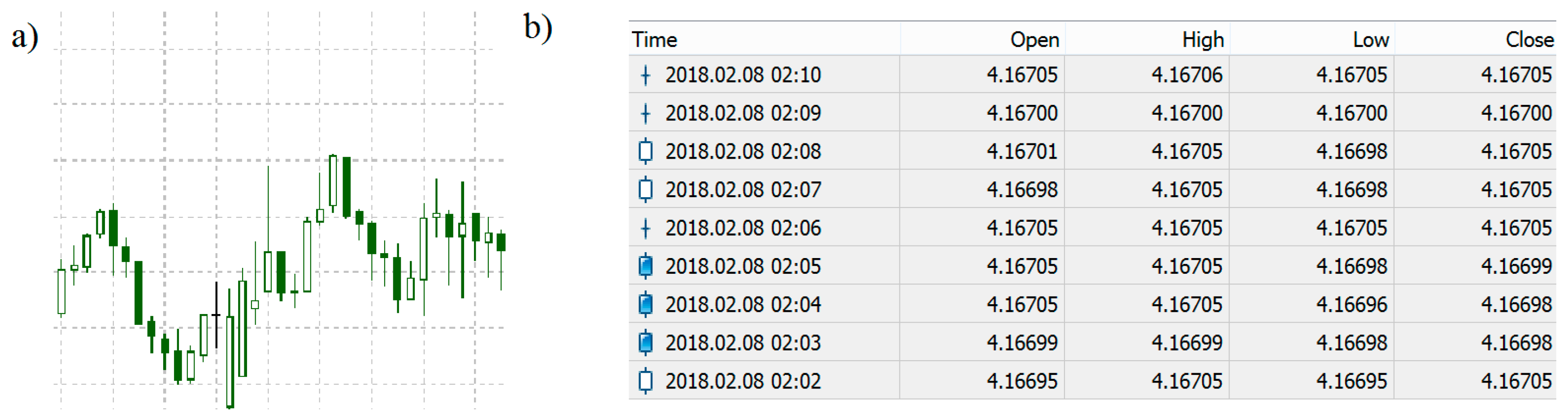
In the candlestick representation, the exchange rate variability in a set time interval is determined by four parameters: the opening price, the closing price and the maximum and minimum price, recorded during the said time period. Figure 1a shows an example of a candlestick chart. With the development of the automated statistical analysis techniques, a method for big data recording was adopted to the stock exchange analyses. It consists of creating a table showing all four parameters of subsequent candles (Figure 1b). This form of data presentation dominates in scientific research and is used to analyze market volatility. In most cases only one candle parameter is used, e.g., the opening price, which further reduces the reliability of the results. Often such data are not called “candlestick”, but e.g., “daily”, “minute”, etc. (Rundo et al. 2019).
It is also good to focus on the close links between the investment practice and the candlestick representation (Gallo 2014). All broker platforms currently use candlestick format to present and analyze data. It is also the only method of testing HFT systems on the most popular currency market platform—MetaTrader (the consequences of this fact are described in Section 4).
4. Disadvantages of the Candlestick Representation
Exchange rates of different financial instruments change with a different variability in time. For example, during a five-minute time period at night, EUR/USD exchange rate fluctuations are several times smaller than those during a five-minute period ensuing right after announcing changes in interest rates by the Federal Reserve System. In candlestick representation this leads to a loss of information about the order and range of occurring changes. As a result, the investor is at risk of wrong conclusions and unfavorable investing decisions. It is particularly important in HFT systems, which can make a few or even a few dozen transactions during the time represented by only one candlestick (Aldridge 2013). It is good to notice that in case of many HFT systems, the time after announcing important economic information is when the most transactions take place, all of them being very quick. Because of this, the analysis of the character of short time changes during a period of intensive trade has a key meaning for both market variability research and investment strategy testing.
4.1. Disadvantages in Context of Statistical Analysis
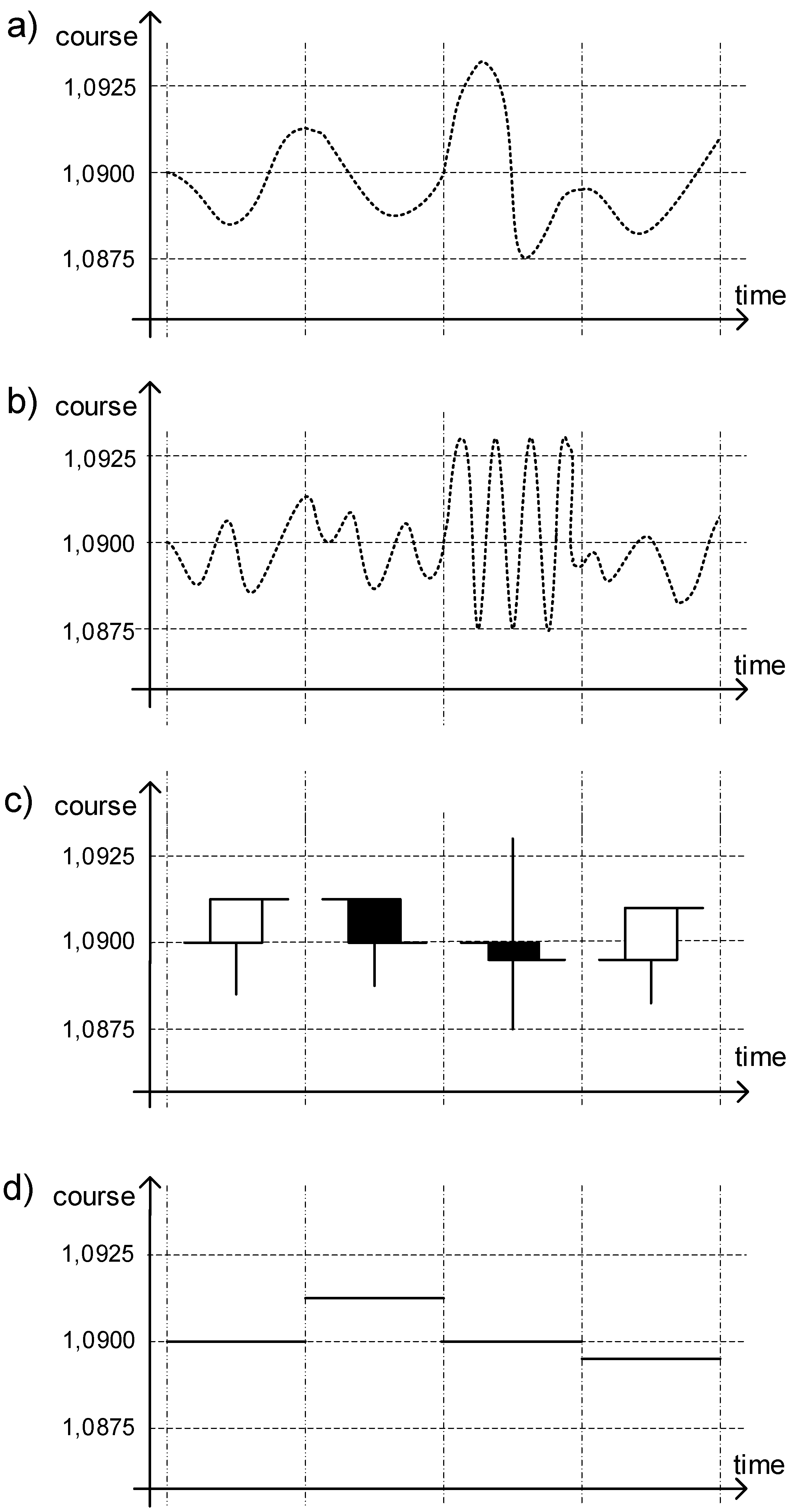
In the vast majority of scientific research authors use data in the form of candlestick charts in order to perform a statistical analysis of the market. The main goal of these studies is usually verification of a particular character of the changes (e.g., effectivity analysis, accordance with the distributions, etc.). Figure 2a,b show two different tick charts, which are represented by identical candles (Figure 2c). One can see that when using a candlestick representation, statistical research can indicate the same result for two different quotations (Figure 2a,b). In case of applying just the opening prices (Figure 2d)—which is the most popular format of historical data—the loss of informative value is even higher.
It is good to notice that the loss of informative value caused by the candlestick representation is dependent on the current frequency and range of the particular changes inside the candle. Because of this fact, it is impossible to assess how much and what kind of information about the price is being lost. Therefore, the process of losing information has a dynamic character which is variable in time. As a result, the influence of using the candlestick representation of input data on the research results cannot be unambiguously assessed. This means that some conclusions from research conducted on candlestick data can be incorrect.
One of the most important research studies pertaining to exchange rates are studies of relations between the course trajectory and a given probabilistic distribution. Wrong assumptions, further applied in real distributions can lead to wrong investment decisions. As an example we can mention the spectacular bankruptcy of the hedging fund founded by two Nobel Prize winners LTCM (Long Term Capital Management). The main reason for the gigantic losses of the fund was assessing the risk by the Value at Risk (VaR), which was based on a false assumption of the return rate distribution compliance with the normal distribution (Jorion 2000).
Example 1.
For the purposes of this experiment, the random number generator (consistent with the normal distribution) generated quotations of instrument X (108,000,000 values corresponding to five years of one second quotations were generated). In order to confirm the correct operation of the generator, the obtained quotations were verified by the Kolmogorov–Smirnov test. With the significance level of 0.05 which is commonly used in economic sciences, the test confirmed that the generated distribution is consistent with the normal distribution:
p value = 0.4756.
The quotations of instrument X are in accordance with the normal distribution, and so the methods using this assumption (such as risk assessment, modelling etc.) can be used. Let us now consider a hypothetical researcher, who does not know the real character of the instrument X’s quotations. They want to verify the following hypothesis:
Hypothesis 1 (H1).
The curse of the instrument X from the last 5 years is in compliance with the normal distribution.
According to the commonly accepted methodology, the researcher uses historical data in the form of one-minute candles (the opening prices only). Only the quotation from the first second of each minute is analyzed, and all transactions occurring “inside” the candle are omitted. As a consequence, from the 108,000,000 registered changes, the researcher analyzes only 1,800,000 quotations. Using the Kolmogorov–Smirnov (Massey 1951) test with the same significance level of 0.05, but for the one-minute opening prices, the researcher discards the hypothesis of the instrument X course compliance with the normal distribution:
p value = 0.008.
The considered example shows that despite the correct selection of statistical tools in the conducted research, the obtained result can be incorrect. The error stems from the use of commonly accepted data formatting (in economics, publications using data in the form of daily, hourly or minute candles prevail).
On many scientific forums, in journals and on conferences, there are disputes pertaining to the selection of proper statistical tools, while a publication describing the proper data format is yet to be found. An answer to the question of the effect of this popular formatting on the quality of forecasts and risk assessment can be crucial for a proper analysis of highly variable financial instruments.
4.2. Disadvantages in the Context of Forecast Interpretation
Historical data analysis is, in many cases, performed in order to identify particular dependencies, for example, investors’ behavioral patterns, occurring statistically more often and being a reaction for a particular situation on a market (e.g., lowering the interest rates, etc.). To describe these kind of dependencies many scientific researchers use neural networks or data mining algorithms. Because of the innate character of those tools (e.g., computational possibilities, etc.), there arises a need for a properly formatted and filtered input data (since high frequency market data can be “noisy”). Yet, in this case as well, most of the researchers use candlestick input data, sometimes even in a truncated form of, for example, daily opening prices (Fischer and Krauss 2018). This kind of approach researches dependencies between the history and parameters of the next candle, in order to build investment decision support tools. However, predicting the parameters of the next candle does not give any possibilities for implementing the results in the investment practice.
Example 2.
Researcher Y used a neural network and daily historical data (opening prices of the daily candle) and obtained very promising results. The network in the testing period shows 80% accuracy in predicting if the next day will end with an increase or a decrease of the course in relation to the opening price. The researcher publishes their work.
Let us now consider an investor who wants to apply the described network in supporting their investment decisions. Construction of a HFT system that makes investment decisions based on suggestions of the neural network should include proper appointment of the TP and SL levels. An investor’s profit depends on those very levels. Network only suggests that the course will be higher or smaller than the opening price. The investor can, therefore, set the TP and SL levels subjectively. Yet, it can happen that some of the transactions are realized on the SL level, the course trajectory changes after some time and the day ends in the way the neural network has predicted. In this case, despite the 80% accuracy of suggestions, the investor can achieve a loss.
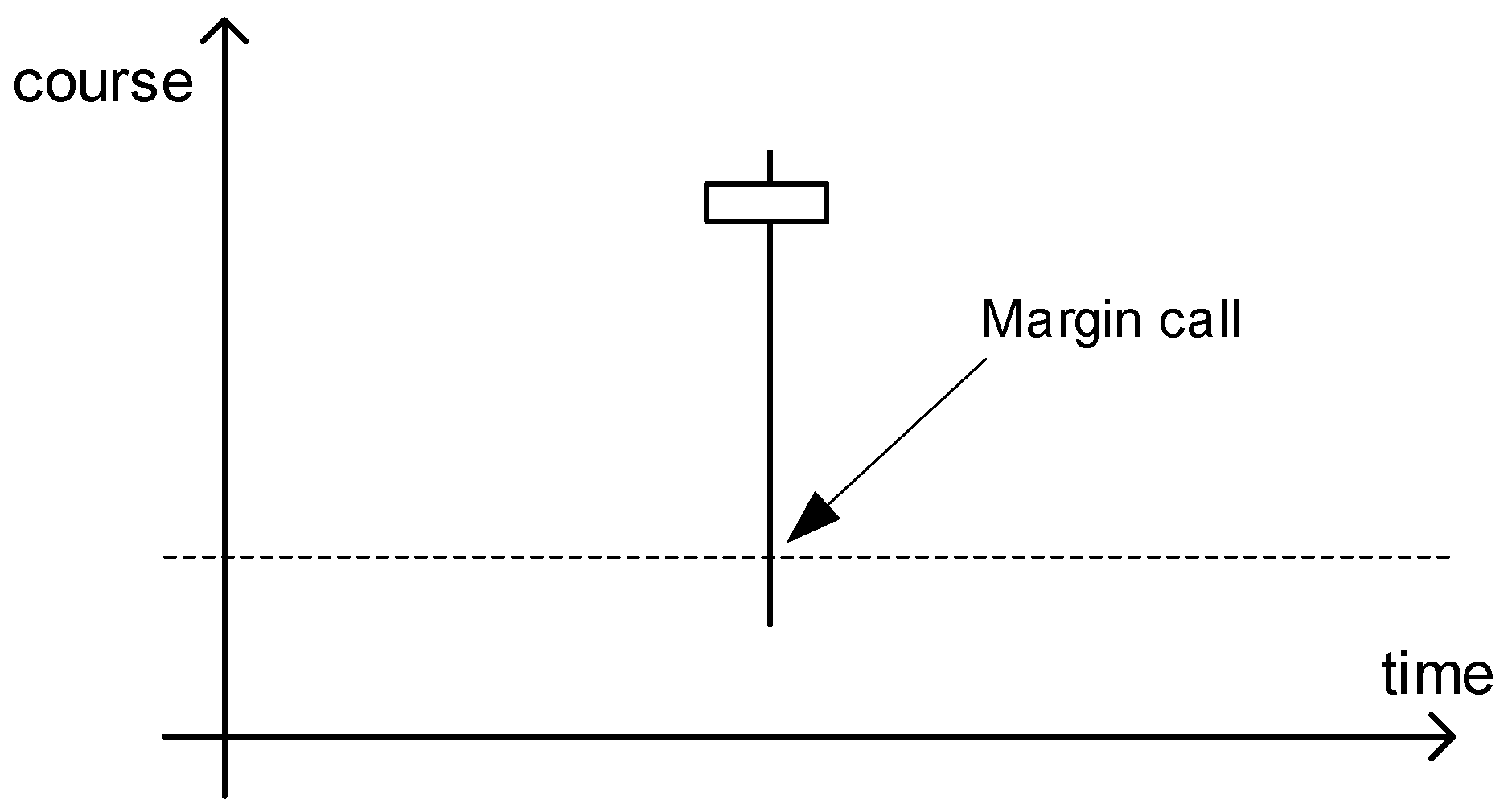
The investor can, of course, resign from setting the TP and SL levels and close the transactions always at the end of the day—this way indeed 80% of the transactions will end with a profit. Despite this conclusion, losses from 20% of the transactions can nominally be significantly higher than the profit from the remaining 80% of transactions. Not setting the SL parameter can have another consequence. Let us consider that the given day is characterized by a high variability in quotations (Figure 3). If the investor will not have enough funds to maintain the position, it will automatically close with zeroing of the investor’s account (and although this would be another “good” forecast, it means a loss of invested capital for the investor).
As from the reasons stated above, the way of using the researched neural network is highly limited. In order to effectively use its results, further research is needed, allowing for an optimal appointment of the TP and SL levels. However, during the research we can obtain that even despite the 80% accuracy, it is impossible to build a strategy allowing for achieving a positive return rate.
4.3. Disadvantages in the Context of HFT Systems Analysis
The development of new technologies allows for trade automation and leads to a rapid increase in the number of transactions made in a short period of time. As an example, on the biggest financial market—the Forex currency market—thanks to using VPS servers, the time of making a bid is counted in milliseconds. Simultaneously, because of the rapid decrease of spreads to the level of tenths of pips, HFT systems can make even a few dozen transactions in one minute. These kind of possibilities open a new space for structure research of the frequently changing market. Using candlestick representation in that kind of research can lead to severe consequences, which are already felt by many investors.
The MetaTrader platform, which is most popular among the investors, allows for testing investment strategies based on historical data (backtest), which is expressed in a candlestick representation with the smallest possible timeframe, equal to one minute. In the Internet we can find many HFT system offers, which are tested based on candlestick data. Analysts and investors also test their strategies based on the MetaTrader strategy tester. However, an analysis using candlestick data is often not very credible and the unaware investor choses a HFT system which is, in fact, not profitable.
Example 3.
Let us now consider an example of verifying the following strategy:
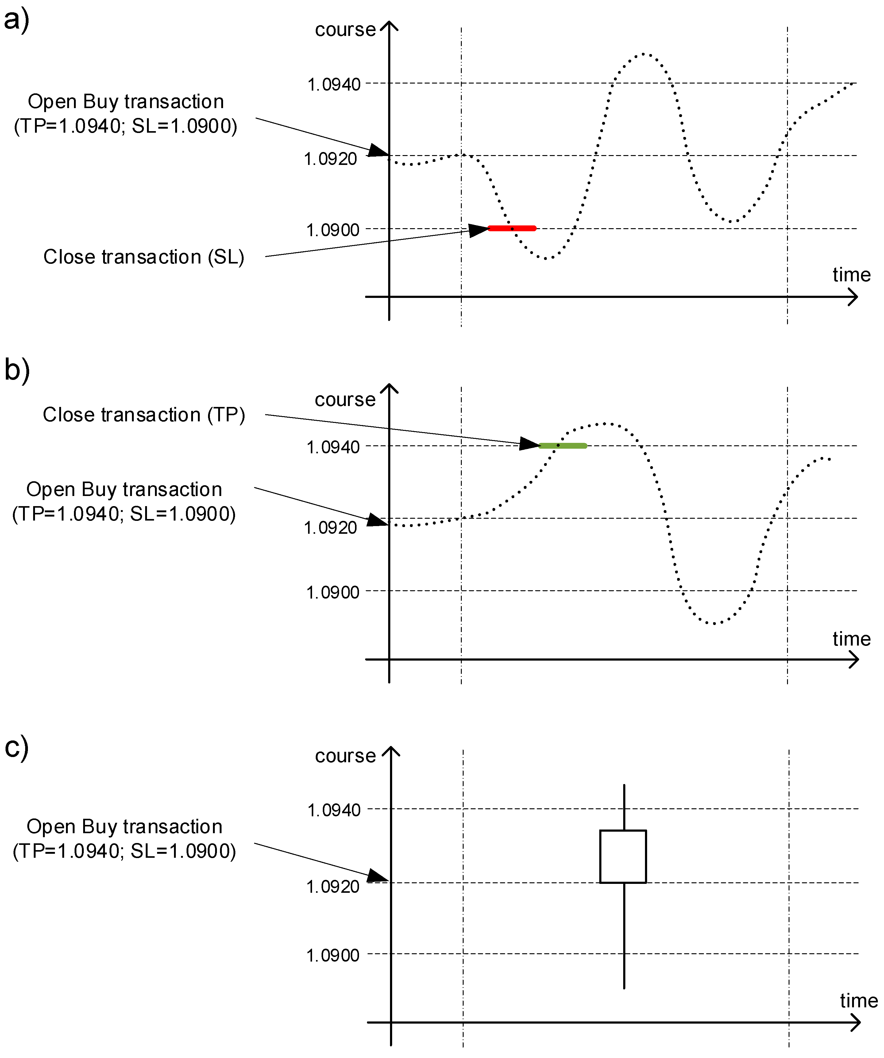
It is easy to notice that in such strategy, the transactions are made alternately, so that the end of one transaction is a signal to make the other one. After performing a backtest, one can assess the ratio between the number of transactions that ended with a profit to the number of all transactions and verify the results of investing in the given time period (return rate, balance fluctuations, maximal drawdown, etc.). Let us assume, that in order to perform the backtest we use a candlestick representation. During the backtest we can encounter candles for which we cannot determine if we obtained a loss or a profit. Figure 4 shows a situation, in which in the moment of occurring a candle already has an open “buy” transaction with parameters TP = 1.0940 and SL = 1.0900. Figure 4a shows a transaction that finishes with a profit, and Figure 4b shows when the same transaction ends with a loss. Yet, both quotations are represented by the same candle (Figure 4c).After each course increase of 20 pips, a “sell” transaction is being opened, with the following parameters: TP = Price − 20 pips, SL = Price + 20 pips. After each course fall of 20 pips, a “buy” transaction is being opened with the following parameters: TP = Price + 20 pips, SL = Price − 20 pips.
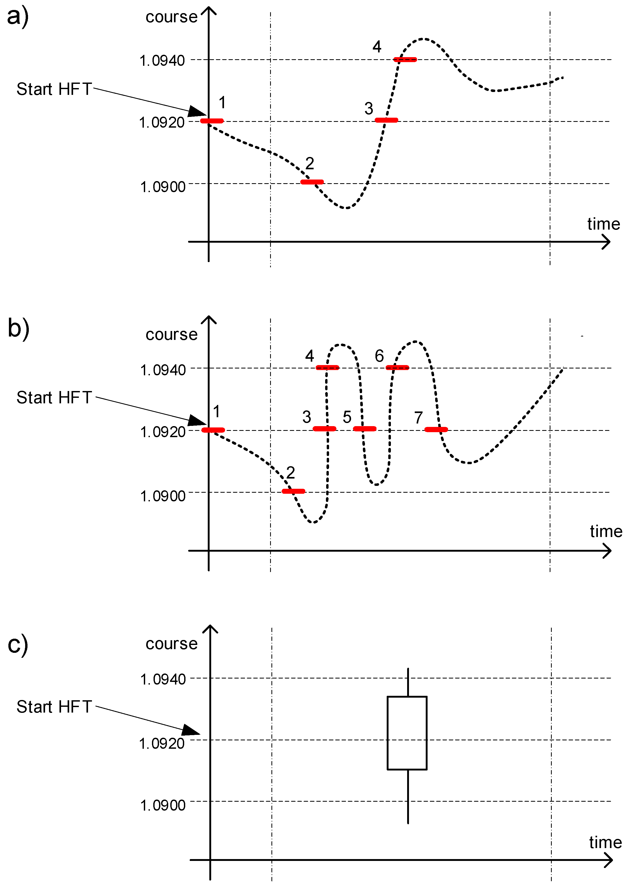
Moreover, in many cases the frequency of changes in unknown and, in consequence, the number of potential transactions made during a single candle is also unknown. Figure 5a presents a possible EUR/USD course trajectory “inside” the candle from Figure 5c. The following points are marked:
- Observation start.
- 20 pips fall—making a “buy” transaction (transaction 1: TP = 1.0900, SL = 1.0880).
- 20 pips rise—ending the transaction 1 with a profit. Making a “sell” transaction (transaction 2: TP = 1.0900, SL = 1.0940).
- 20 pips rise—ending the transaction 2 with a loss. Making a “sell” transaction (transaction 3: TP = 1.0920, SL = 1.0960).
During the observation, the investor’s balance changed (one transaction ended with a profit and the second one with a loss). Figure 5b depicts another possibility of the course trajectory inside the same candle, where the following points were marked:
- Observation start.
- 20 pips fall—making a “buy” transaction (transaction 1: TP = 1.0900, SL = 1.0880).
- 20 pips rise—ending the transaction 1 with a profit. Making a “sell” transaction (transaction 2: TP = 1.0900, SL = 1.0940).
- 20 pips rise—ending the transaction 2 with a loss. Making a “sell” transaction (transaction 3: TP = 1.0920, SL = 1.0960).
- 20 pips fall—ending the transaction 3 with a profit. Making a “buy” transaction (transaction 4: TP = 1.0940, SL = 1.0900).
- 20 pips rise—ending the transaction 4 with a profit. Making a “sell” transaction (transaction 5: TP = 1.0920, SL = 1.0960).
- 20 pips fall—ending the transaction 5 with a profit. Making a “buy” transaction (transaction 6: TP = 1.0940, SL = 1.0900).
With this kind of course trajectory, during one minute one of the transactions ended in a loss, yet four others ended with a profit, which means that the investor’s balance has greatly increased.
The scale of the presented phenomenon depends on the appointed timeframe. However, taking into account the characteristics of some financial instruments popular nowadays (e.g., quotations of currency pairs), and the way the majority of HFT systems perform during high trade, such phenomena can occur quite commonly, even though one can use the smallest and vastly applied one-minute time frame. Along with the implementation of IT solutions on the markets, the problem will get more and more severe, and wrongly tested strategies will generate significant loses on investors balances.
5. Binary-Temporal Approach
Despite the size of data, in order to properly test investment strategies and to perform basic statistical analysis, it is enough to use tick data—most of the modern computers are able to compute such kinds of inputs. However, in case of many different methods, using unprocessed tick data can be difficult or even prevent an effective course analysis. In Section 2 we have proved that accurately chosen course representation should comprise properly filtered data. Taking into account the structure of e.g., neural networks, using unprocessed tick data greatly complicates or even prevents an effective market analysis. On the other hand, using data in candlestick representation leads to results that are unreliable (Example 4) and hard to interpret (Example 3). A proper representation, as the author sees it, should eliminate changes of a very small range. In order to do so, a binary representation was proposed (Stasiak 2016), which was inspired by the sadly forgotten point-symbolic method (De Villiers 1933). The main idea of this representation is to show changes on the market with the use of a binary sequence. The so-called binary-temporal course representation (Stasiak 2017a, 2018) is a generalization of the binary representation. The binary-temporal representation, similar to the candlestick representation, includes information about the change range and duration. Yet, it is characterized by higher accuracy (i.e., possibility of an assessment) and interpretation ease.
5.1. Binary-Temporal Representation
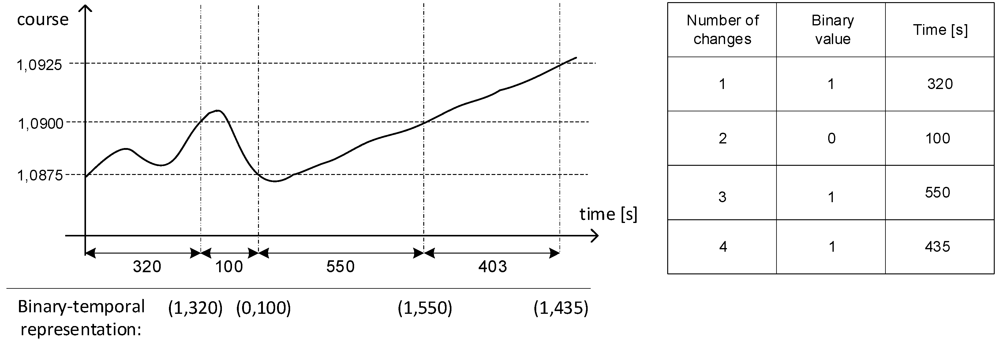
In order to present data in the binary-temporal representation, the so-called binarization algorithm is used. This algorithm assigns upper and lower change limits for the initial course value. The limits equal the course increase and decrease by given discretization unit (DU). The binarization algorithm also registers the initial time. If the course falls below the lower limit, the algorithm assigns each change i two values—the binary value zero ( = 0) and duration of this change in seconds (). In case of the price increase above the upper limit, the algorithm assigns the i-th change the binary value of one ( = 1) and again, the duration of the change in seconds (). In the next steps the algorithm appoints new limits, depending on the last registered course change, and counts the time in dependence to the duration of each previous change. In effect, we obtain a representation of the currency pair exchange rate in form of a sequence:
where n is the number of changes observed in the researched time period. Figure 6 shows an overview of the discretization algorithm’s performance, in case of constructing a binary-temporal representation. Figure 6 also depicts a tabular form of the binary-temporal representation.
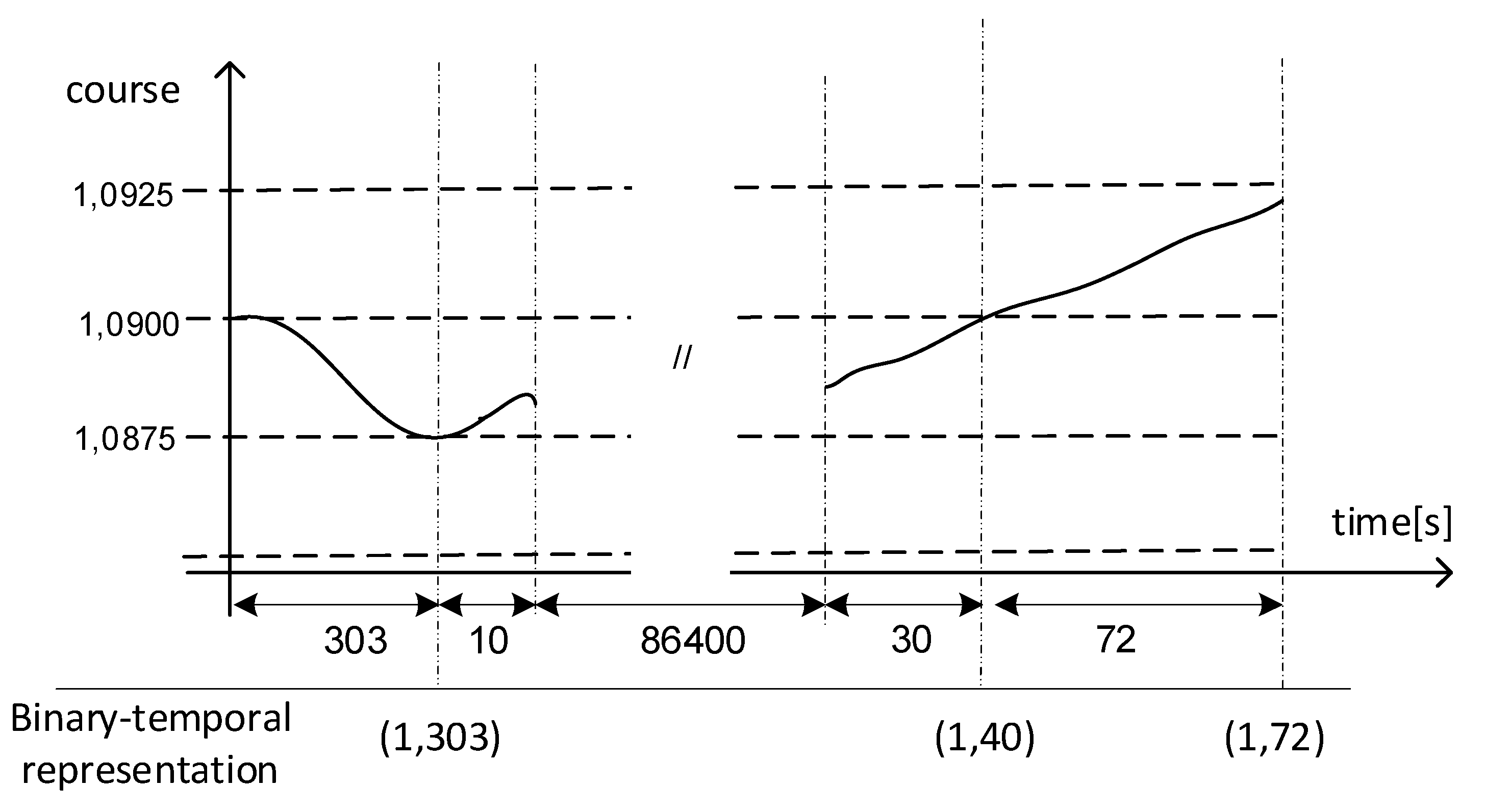
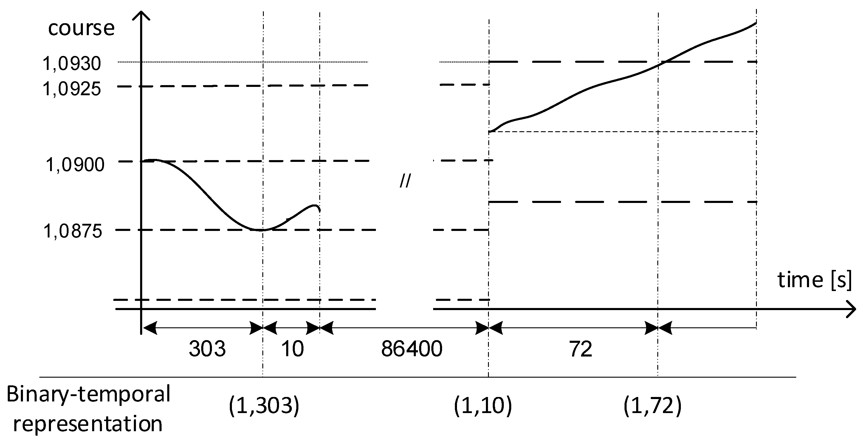
On a financial market, after opening the quotations after some kind of a break (i.e., after a weekend, holidays), a so-called “price gap” can appear. Figure 7 shows this kind of situation. The discretization algorithm in such a scenario does not include the time, in which the market is closed. In the analyzed example, the duration of the change equals 1 min. In case of exceeding the discretization unit after a price gap (Figure 8), the given change is assigned a binary value which would have been reached (in the analyzed example—an increase). Next, the algorithm registers the time and the next change in respect to the price of the first quotation after the gap—the course has to rise or fall by one discretization unit from the first quotation after the gap.
5.2. Application of the Binary-Temporal Representation
The binary-temporal representation can be used in order to effectively model exchange rates. The appointed discretization unit stands as a filter which eliminates changes of a very small range. As an example, using the smallest discretization unit we obtain tick data but without the identical quotations repeated several times. Appointing higher values of the discretization units leads, on the other hand, to elimination of information about the changes of a smaller range, including the noise. With the increase of the applied discretization unit, the loss of informative value is getting higher (Stasiak 2018). However, the most important thing is that contrary to the candlestick representation, the level of the informative value can always be specified, since each change of the size bigger than the DU will not be omitted. This stands as the most important difference between the binary-temporal and candlestick representation.
In the context of analyzing a particular financial instrument, research of a vast spectrum of discretization units is justified. Based on this, one can appoint the change range limit that limits the noise and one can chose optimal discretization unit for the given market.
Using the binary representation allows for a renewed verification of many assumptions and hypotheses encountered in scientific research since way back, which were not credibly verified because of the defects of the candlestick representation (or its short version, e.g., only the opening prices). That kind of research can be burdened with significant errors (Examples 3–5).
Example 4.
Even today, there are disputes among researchers regarding whether to accept or to discard the market effectiveness hypothesis or the random walk hypothesis. Adopting those hypotheses assumes the impossibility of predicting the future quotations based on historical course trajectory data and its application in technical analysis methods. In many papers, in order to verify those hypotheses, statistical testing is used, which is meant to detect potential statistical dependencies between the historical and future quotations. However, in this kind of research the candlestick representation is used, e.g., daily data. In previous examples we have proved that research based on data given in the candlestick representation may not be credible. Let us now consider using the binary representation. Employing test sets that verify the existence of possible dependencies in binary sequences (e.g., tests suggested by NIST (Bassham et al. 2010) for testing pseudo-random number generators in cryptographic modules) for a given discretization unit allow to verify the character of the data. If the data have an unpredictable character the market effectiveness hypothesis is proved. If the data are more or less dependent, the technical analysis methods are justified.
The second difference between the binary and candlestick representation is the interpretation ease of the results and possibility of direct application in investment practice, in the binary representation a change can be associated with a transaction of a given TP and SL parameters. In case of a more probable increase, the TP level describes a change of a value 1, and SL describes the occurrence of 0 (contrary to the case of a more probable decrease). In this case, the probability distribution of the future change direction is equal to the probability distribution of profits (Piasecki and Stasiak 2019). Example 5 corresponds with the Example 3 and presents the differences in application possibilities of the research results based on the candlestick and binary representation, respectively.
Example 5.
Researcher X proposed a neural network that analyses historical data in form of a binary-temporal representation, for the discretization unit of DU = 20 pips. The network indicates the direction of the next change with an 80% correctness (0 for a fall and 1 for a rise).
Let us now consider an investor, who wants to create an HFT system based on this research. The construction of a HFT system should include a proper appointment of the TP and SL levels. In case of the binary representation, those levels for the purchase transaction (where the future increase is more probable—value 1 in binary-temporal representation) are equal to:
and for the sale transaction (where the future decrease is more probable—value 0 in the binary-temporal representation) the levels are as follows:
With this method of appointing the TP and SL levels, in case of a correct guess, the transaction ends on the TP level, and in the case of a wrong guess—on the SL level. Because of this fact, the correctness of guesses is equal to the probability of achieving a profit in a single transaction.
TP = Price + 20 pips,
SL = Price − 20 pips,
SL = Price − 20 pips,
TP = Price − 20 pips,
SL = Price + 20 pips.
SL = Price + 20 pips.
As a consequence, based on the proposed neural network, 80% of transactions made will probably end with a profit, and 20% will end with a loss. In such a scenario there exists a possibility of an accurate assessment of profits generated by the HFT system, constructed based on this network.
The HFT system presented in Example 3 can be easily verified with use of historical data in a binary representation: the profit is achieved with each increase (1) that follows a fall (0), or with each fall (0) that follows an increase. A loss occurs in contrary situations. In Example 5 a hypothetical use of a neural network was presented. The network acts as a black box, i.e., as a system with unknown decision making rules. Let us consider the opportunities that are offered by using binary-temporal representation of a course.
Example 6.
Researcher X decided to analyze an investor’s reaction to the case of a rapid price change equal to five discretization units, in time no longer than one hour. When using the binary temporal representation, the condition for such a behavior pattern can be formulated as follows:
This kind of detailed definition of behavior pattern allows for a statistical analysis of the investor’s reaction expressed in form of the next change in quotations - εi+1. If the given reaction, e.g., an increase, statistically occurs more often, it can stand as a basis to support investment decisions or to build an HFT system.
Using the binary-temporal representation as a format for tick data fulfills its main purpose, that is the noise elimination. The binary-temporal representation can, therefore, effectively substitute the candlestick representation and its derivatives. Contrary to the candlestick representation, the binary-temporal representation allows for a precise description of the level of information loss about the course trajectory (i.e., about the changes smaller than the discretization unit).
Using a binary-temporal representation results in the possibility of constructing so-called state models, in which the course is depicted as a transition process between states defined as investor’s behavior patterns (an approach analogous to the one presented in Example 6) (Stasiak 2018). This kind of approach allows for appointing probability distributions of the course variations. Along with the binary-temporal representation, complex wave detection algorithms were created for the market, which empirically proved the existence of statistical dependencies between ensuing waves (which is the main assumption of Elliott’s theory). By applying the binary-temporal representation the author also proved the possibility of forecasting changes of a given range with the accuracy of over 68% for the researched financial instruments on the Forex currency market (Stasiak 2017b).
To sum up, we can conclude that in comparison to the candlestick representation, the binary-temporal representation has the following advantages:
- Allows one to determine the range of registered trajectory changes. All changes higher than the assumed discretization unit are included in the analysis;
- Allows for a credible assessment of the prediction results;
- Allows for a reliable testing of investment strategies.
6. Conclusions
In the article, the main focus was placed on the problem of information loss for the historical data presented in candlestick representation, which is difficult to assess and verify in time. This problem is often marginalized in existing subject literature. The commonness of the candlestick representation causes this data format to be applied without any consideration in case of modelling, performing statistical analyses or using other predictive methods. Candlestick data are used for searching for dependencies, researching the exchange rate trajectory or testing developed HFT systems. The author suggests that using this data format can negatively influence the results of statistical analysis. As a consequence, calculations in many papers, despite a properly executed analysis, can still lead to false conclusions. This kind of influence was not yet researched in the subject literature.
The article also highlights the dangers caused by using candlestick representation by analysts and investors in the investment practice, especially in the context of highly popular HFT systems. The fact that even the biggest broker platforms created some dedicated tools for testing HFT strategies which are based only on the candlestick representation (MetaTrader) shows how crucial the problem is for both scientific research and the investment practice. The article emphasizes the discrepancies between the two.
The article also indicates the problem of discrepancy between scientific research and the investment practice. Because of this, many theoretical solutions, despite the formal appropriateness, lead, in practice, to financially ineffective decisions. The author hopes that this paper will draw attention to the need for using new representations, alternative to the candlestick one, in order to model changes on the high frequency markets.
In the candlestick representation, the duration of a candle is constant, and the described time period is a for quotations “timing”. In the binary-temporal representation, the base for timing is the change in quotations of the size of the assumed discretization unit. In the binary-temporal solution, the time plays the role of an additional parameter, assigned to a single “moment”, which informs about the change duration and carries a prognostic value. The approach taken in the binary-temporal representation allows for an analysis of all changes greater or equal to the discretization unit, i.e., all data significant for a given forecast strategy. Therefore, the proposed representation acts as a filter that cancels the noise made by the values smaller than the discretization unit.
The article introduces a new method for the exchange rate course representation, which allows for an effective filtering of the noise with a simultaneous retention of key information that is crucial for effective market variability analysis. Proposed binary-temporal representation leads to a simple method of historical data formatting, on a given accuracy level. Using the introduced representation allows for a credible statistical analysis of possible dependencies. A great advantage of the binary-temporal representation is the possibility of an easy and unambiguous translation of the scientific research results to the investment practice.
Funding
This research received no external funding.
Conflicts of Interest
The author declares no conflict of interest.
References
- Aldridge, Irene. 2013. High-Frequency Trading: A Practical Guide to Algorithmic Strategies and Trading Systems. Hoboken: Wiley. [Google Scholar]
- Alonso-Monsalve, Saúl, Andrés L. Suárez-Cetrulo, Alejandro Cervantes, and David Quintana. 2020. Convolution on Neural Networks for High-Frequency Trend Prediction of Cryptocurrency Exchange Rates Using Technical Indicators. Expert Systems with Applications 149: 113250. [Google Scholar] [CrossRef]
- Bassham, Lawrence E., III, Andrew L. Rukhin, Juan Soto, James R. Nechvatal, Miles E. Smid, Elaine B. Barker, Stefan D. Leigh, Mark Levenson, Mark Vangel, David Banks, and et al. 2010. Sp 800-22 Rev. 1a. A Statistical Test Suite for Random and Pseudorandom Number Generators for Cryptographic Applications. Gaithersburg: National Institute of Standards & Technology. [Google Scholar]
- Burgess, Gareth. 2010. Trading and Investing in the Forex Market Using Chart Techniques. Chichester: John Wiley & Sons. [Google Scholar]
- De Villiers, Victor. 1933. The Point and Figure Method of Anticipating Stock Price Movements Complete Theory & Practice. A Reprint of the 1933 Edition Including a Chart on the 1929 Crash. New York: Windsor Books. [Google Scholar]
- Fischer, Thomas, and Christopher Krauss. 2018. Deep Learning with Long Short-Term Memory Networks for Financial Market Predictions. European Journal of Operational Research 270: 654–69. [Google Scholar] [CrossRef] [Green Version]
- Frost, Alfred John, and Robert Rougelot Prechter. 2014. Elliott Wave Principle: Key to Market Behavior. Gainesville: New Classics Library. [Google Scholar]
- Gallo, Crescenzio. 2014. The Forex Market in Practice: A Computing Approach for Automated Trading Strategies. International Journal of Economics & Management Sciences 3. [Google Scholar] [CrossRef]
- Jorion, Philippe. 2000. Risk Management Lessons from Long-Term Capital Management. European Financial Management 6: 277–300. [Google Scholar] [CrossRef]
- Kirkpatrick, Charles D., and Julie R. Dahlquist. 2010. Technical Analysis: The Complete Resource for Financial Market Technicians, 2nd ed. Upper Saddle River: FT Press. [Google Scholar]
- Li, Yang, Wanshan Zheng, and Zibin Zheng. 2019. Deep Robust Reinforcement Learning for Practical Algorithmic Trading. IEEE Access 7: 108014–22. [Google Scholar] [CrossRef]
- Lo, Andrew W., Harry Mamaysky, and Jiang Wang. 2000. Foundations of Technical Analysis: Computational Algorithms, Statistical Inference, and Empirical Implementation. The Journal of Finance 55: 1705–65. [Google Scholar] [CrossRef] [Green Version]
- Logue, Dennis E., and Richard James Sweeney. 1977. “White –noise” in Imperfect Markets: The Case Study of the Franc/Dollar Exchange Rate. The Journal of Finance 32: 761–68. [Google Scholar] [CrossRef]
- Massey, Frank J. 1951. The Kolmogorov-Smirnov Test for Goodness of Fit. Journal of the American Statistical Association 46: 68–78. [Google Scholar] [CrossRef]
- Neely, Christopher J., and Paul A. Weller. 2011. Technical Analysis in the Foreign Exchange Market. Federal Reserve Bank of St. Louis Working Paper. Available online: https://papers.ssrn.com/sol3/papers.cfm?abstract_id=1734836 (accessed on 1 August 2020).
- Piasecki, Krzysztof, and Michał Dominik Stasiak. 2019. The Forex Trading System for Speculation with Constant Magnitude of Unit Return. Mathematics 7: 623. [Google Scholar] [CrossRef] [Green Version]
- Rundo, Francesco, Francesca Trenta, Agatino Luigi di Stallo, and Sebastiano Battiato. 2019. Grid Trading System Robot (GTSbot): A Novel Mathematical Algorithm for Trading FX Market. Applied Sciences 9: 1796. [Google Scholar] [CrossRef] [Green Version]
- Schlossberg, Boris. 2012. Technical Analysis of the Currency Market: Classic Techniques for Profiting from Market Swings and Trader Sentiment. Hoboken: John Wiley & Sons, Inc. [Google Scholar] [CrossRef]
- Stasiak, Michał Dominik. 2016. Modelling of currency exchange rates using a binary representation. In Proceedings of 37th International Conference on Information Systems Architecture and Technology—ISAT 2016. Cham: Springer, vol. 524, pp. 153–61. [Google Scholar] [CrossRef]
- Stasiak, Michał Dominik. 2017a. Analysis of the EUR/USD Exchange Rate in Binary-Temporal Representation. Research Papers in Economics and Finance 2: 39–45. [Google Scholar] [CrossRef]
- Stasiak, Michał Dominik. 2017b. Modelling of currency exchange rates using a binary-wave representation. In Proceedings of 38th International Conference on Information Systems Architecture and Technology—ISAT 2017. Cham: Springer, vol. 657, pp. 27–37. [Google Scholar] [CrossRef]
- Stasiak, Michał Dominik. 2018. A study on the influence of the discretisation unit on the effectiveness of modelling currency exchange rates using the binary-temporal representation. Operations Research and Decisions 28: 57–70. [Google Scholar] [CrossRef]
- Vezeris, Dimitrios, Themistoklis Kyrgos, and Christos Schinas. 2018. Take Profit and Stop Loss Trading Strategies Comparison in Combination with an MACD Trading System. Journal of Risk and Financial Management 11: 56. [Google Scholar] [CrossRef] [Green Version]
- Yao, Jingtao, and Chew Lim Tan. 2000. A Case Study on Using Neural Networks to Perform Technical Forecasting of Forex. Neurocomputing 34: 79–98. [Google Scholar] [CrossRef] [Green Version]
Figure 1.
Candlestick representation of the course: (a) plot (b) data format.

Figure 2.
Data representation: (a) tick data version 1 (b) tick data version 2 (c) candlestick representation—one-minute candles (d) short candlestick representation (opening prices)—one-minute candles.
Figure 2.
Data representation: (a) tick data version 1 (b) tick data version 2 (c) candlestick representation—one-minute candles (d) short candlestick representation (opening prices)—one-minute candles.

Figure 3.
An increase candle with a significant fall “inside”.

Figure 4.
Different possible course trajectories (a,b) “inside” the same candle (c).

Figure 5.
Different possible course trajectories and number of transactions (a,b) “inside” the same candle (c).
Figure 5.
Different possible course trajectories and number of transactions (a,b) “inside” the same candle (c).

Figure 6.
Performance of the algorithm for constructing binary-temporal representation for the discretization unit of 20 pips.
Figure 6.
Performance of the algorithm for constructing binary-temporal representation for the discretization unit of 20 pips.

Figure 7.
Binary-temporal representation algorithm’s performance during the session opening/closure.
Figure 7.
Binary-temporal representation algorithm’s performance during the session opening/closure.

Figure 8.
Binary-temporal representation algorithm’s performance during a price gap.

© 2020 by the author. Licensee MDPI, Basel, Switzerland. This article is an open access article distributed under the terms and conditions of the Creative Commons Attribution (CC BY) license (http://creativecommons.org/licenses/by/4.0/).
Share and Cite
MDPI and ACS Style
Stasiak, M.D. Candlestick—The Main Mistake of Economy Research in High Frequency Markets. Int. J. Financial Stud. 2020, 8, 59. https://0-doi-org.brum.beds.ac.uk/10.3390/ijfs8040059
AMA Style
Stasiak MD. Candlestick—The Main Mistake of Economy Research in High Frequency Markets. International Journal of Financial Studies. 2020; 8(4):59. https://0-doi-org.brum.beds.ac.uk/10.3390/ijfs8040059
Chicago/Turabian StyleStasiak, Michał Dominik. 2020. "Candlestick—The Main Mistake of Economy Research in High Frequency Markets" International Journal of Financial Studies 8, no. 4: 59. https://0-doi-org.brum.beds.ac.uk/10.3390/ijfs8040059
Note that from the first issue of 2016, this journal uses article numbers instead of page numbers. See further details here.