Article

Non-Performing Loans for Italian Companies: When Time Matters. An Empirical Research on Estimating Probability to Default and Loss Given Default

by
Giuseppe Orlando
1,2,* and
Roberta Pelosi
1
1
Department of Economics and Finance, University of Bari “Aldo Moro”, Via C. Rosalba 53, 70124 Bari, Italy
2
Department of Applied Mathematics, Universidad de Jaén, Campus Las Lagunillas, Avda. Antonio Pascual Acosta, 23071 Jaén, Spain
*
Author to whom correspondence should be addressed.
Int. J. Financial Stud. 2020, 8(4), 68; https://0-doi-org.brum.beds.ac.uk/10.3390/ijfs8040068
Submission received: 18 September 2020 / Revised: 1 November 2020 / Accepted: 3 November 2020 / Published: 9 November 2020
(This article belongs to the Special Issue Alternative Models and Methods in Financial Economics)

Abstract

:
Within bank activities, which is normally defined as the joint exercise of savings collection and credit supply, risk-taking is natural, as in many human activities. Among risks related to credit intermediation, credit risk assumes particular importance. It is most simply defined as the potential that a bank borrower or counterparty fails to fulfil correctly at maturity the pecuniary obligations assumed as principal and interest. Whenever this happens, a loan is non-performing. Among the main risk components, the Probability of Default (PD) and the Loss Given Default (LGD) have been the subject of greater interest for research. In this paper, logit model is used to predict both components. Financial ratios are used to estimate the PD. Time of recovery and presence of collateral are used as covariates of the LGD. Here, we confirm that the main driver of economic losses is the bureaucratically encumbered recovery system and the related legal environment. The long time required by Italian bureaucratic procedures, simply put, seems to lower dramatically the chance of recovery from defaulting counterparties.
JEL Classification:
G18; G21; G32; G38; H55

1. Introduction

In recent years, there has been an impressive development of loans characterized by difficult or uncertain degree of recoverability, defined as non-performing loans. Several factors have contributed to the growth of these “problematic” credits in balance sheets of European creditors, mainly related to the recession triggered out by the collapse of so-called sub-prime mortgages, American real estate financing and the subsequent international crisis of structured finance products. This recession has had heavy consequences even for the European economic system, and in countries such as Italy, where the business funding is mainly supplied by credit institutions, the economic difficulties of underlying borrowers could not fail to influence banking activity, leading to a significant increase in credit risk. The recent economic and financial crisis in Europe has led to progressive deterioration in credit quality and to the consequent immobilization of financial resources, which could, conversely, be used in granting new loans for economic development. To manage this problem and restore the sound and prudent management of credit institutions, it is necessary to speed up the enactment process of regulatory measures. Regulation of the European banking system is still facing a harmonization process that will promote comparability between Member States on this matter, as well as increasing financial stability.
The purpose of this paper is to fit a logit model to estimate PD and LGD for a dataset of Italian firms, where PD depends on the creditworthiness of the debtor, generally estimated on the basis of the economic and financial situation of the debtor, and LGD depends on the nature of loan and on any guarantees that assist it where recovery time is typically given. Here, we maintain that, while risk drivers for LGD levels are several, in our study, time is more important than seniority and guarantees.
The structure of this paper is as follows. Section 2 describes the Italian society and the business environment. Section 3 describes the regulatory framework, the binary and ordered logit models used for computing the PD and LGD, respectively. Section 4 shows the experimental results obtained with both models. Section 5 discusses the results in light of current literature. Section 6 draws some concluding remarks and recommendations.

2. Putting Things in Their Context: An Overview of Italy

2.1. Italian Society and Business Environment

The Italian economy, as well as the society, is affected by a long lasting malaise. Most social spending is for subsidizing an unfair pension system that allowed million of people to enjoy a disproportionate (in terms of paid contributions) lifelong rent. In fact, 28% of social protection expenditure on GDP, 48.8% is for pensions (data refer to 2017, the latest available for a European comparison); in relation to GDP, the Italian welfare expenditure is above the European average (26.8%) but lower than that of France which is at the top of the ranking with 31.7%. Among the risks included in social protection, the most burdensome for almost all countries is old age, which absorbs 40.5% of the benefits provided in the EU in 2017; only Ireland and Germany are exceptions. Italy far exceeds the European average share, but at the top of the ranking are Greece (53.2%), Romania (51.8%) and Portugal (50.7%). On the other hand, Ireland, which devotes less than a third of the services provided (31.8%), Luxembourg (32.0%) and Germany (32.2%) stand out for the lowest spending shares Istat (2020). Italian trade unions represent “privileged” workers (i.e., public servants and old workers who enjoy protected contracts) and pensioners Chiarini (1999). Among the biggest trade unions, the absolute majority of the members of the CGIL and CISL and a quarter of those of the UIL are retired. That represents a much higher percentage than in the rest of Europe, where retired members are on average 10%, with peaks of 15% in some countries. Throughout Germany, 1.7 million pensioners are registered in the trade unions, which is just under half of the 3 million pensioners who are registered with the CGIL alone. In Italy, there are so many pensioners registered with trade unions that our country dominates without contrast the FERPA, the European union of pensioners: out of 10 million members from all over the continent, as many as 6 million are Italian (for this reason, it is now fifteen years that the secretary of FERPA is always Italian) De Luca (2017).
This is compounded by a “non-meritocratic, business environment that feeds back into a low familiarity with ambitious entrepreneurship and a rather closed culture” Sanders et al. (2020). The Bank of Italy reported additional elements to the explanation as to why Italy from the most dynamic European country in the post World War II became a slow-motion economy in the last decades Bugamelli et al. (2018). Essentially, they are ageing, tax evasion, quality and efficacy of the bureaucracy, quality and competitiveness of market services (especially for professional services), inefficacy of contracts enforcement and slowness of court proceedings.
Barone and Cingano (2011), by using OECD’s Product Market Regulation (PMR) indicators, report thated a high degree of restrictiveness in service regulation industries significantly affects value-added, productivity and exports of those industries (typically manufacturing) who use those services as inputs. Several studies confirm that low regulatory burden favors more productive firms Andrews and Cingano (2014); Arnold et al. (2011) and that high regulatory burden reduces investments in knowledge-based capital firms Andrews et al. (2015). A reduction in PMR indices, should be aimed to reduce monopolistic rents, favoring competition and entrants of new firms Bartelsman et al. (2009); Bravo-Biosca et al. (2016). This is particularly true for ICT where labor market and services regulation are key factors for productivity growth and for differences in them Van Reenen et al. (2010) so that strict regulation has a deterrent effect on ICT Barrios and Burgelman (2008).
Incumbents oppose markets and take control of productive assets Rajan and Zingales (2004). The so-called acquired rights and legitimate expectations make the country sclerotic so that, even state property concessions for beaches are impossible to reform. Among the many infringement procedures launched by the EU against Italy, the next could come shortly, given that the extension of tenders for bathing concessions until 2033 is contrary to the European Bolkestein directive (2006/123/EC) which requires the liberalization of services in the internal market of the EU. By May 2017, the Member States should have banned the concessions issued over the years by local authorities, giving the possibility to open a commercial activity on a public area to all European citizens, without limit of nationality, in any country of the EU. In Italy, the number of bathing concessions grows in the face of negligible rents. In 2016, the state collected just over 103 million Euro from concessions against a turnover estimated by Nomisma of 15 billion Euro per year Muroni (2019). However, led by innovative leadership (Bersani reforms, Bentivogli 2009; Fucci and Fucci 1999; Violati 2001) and pushed by the economic crisis, Italy introduced changes aimed at increasing competition in product and service sectors to bridge the gap between the country’s PMR index and the OECD average Bugamelli et al. (2018).
Judiciary system and legal environment are also responsible for allowing the firms to operate efficiently at their optimal scale Laeven and Woodruff (2004); Rajan et al. (2001). This holds true especially for firms with high proportion of intangible assets, like intellectual capital and knowledge assets, which are fundamental factors of innovation Rajan et al. (2001). Burdensome court proceedings and slow trial length affect negatively the supply of credit to households Fabbri (2010) and firms Jappelli et al. (2005).

2.2. Bankruptcy Law

The bankruptcy law was first introduced into the Italian legal system by the Royal Decree of 16 March 1942, n. 267, and had a mainly sanctioning function against the entrepreneur, considered a deplorable subject. In the early 2000s, on the verge of a deep and global economic crises, Italy found itself managing the business crisis with outdated and ineffective legislation. The Legislative Decree 9 January 2006, n. 5 was a first attempt to reform the matter. The major novelty was the introduction of art. 104, which, following the so-called “virtuous practices” of the court, tried, on the one hand, to avoid the fragmentation of the liquidation procedure, through diversified and often uncoordinated operations, and, on the other hand, to manage an uncontrolled expansion of time and costs Panzani (2012).
Prior to the reform, the liquidation activity began with the decree of enforceability of the passive state and the sales took place according to the model of the sale by forced expropriation. As regards the liquidation in the broad sense (such as conservation actions of the assets and the recovering, compensatory actions) little or nothing was regulated. It was common, therefore, that the costs of the entire procedure would far exceed the assets and that this would be noticed only after the procedure was completed. Therefore, while the reform of 2006 maintained the original structure of the law, the legislator, in his illustrative report to clarify the inspiring purposes of the enabling law, intended to bring a change of course accelerating and simplifying the procedure. This was by means of more suitable and rapid tools, to ensure maximum satisfaction of the creditors.
However, while the premise of reform was clear, in daily practice, it was not possible to obtain the same effects of accelerating and streamlining the procedure as hoped. Therefore, various modifications were necessary, especially as regards the liquidation program. Thus, a mini-reform ensued with the Law no. 192 of 20 August 2015 and the Law no. 19 of 30 June 2016 giving an additional impetus towards a prompt definition of bankruptcy procedures Sandulli and D’Attorre (2016).

3. Materials and Methods

3.1. Non-Performing Exposure and Regulation

The centrepiece of technical regulations and harmonized definitions of non-performing exposures is the European Banking Authority (EBA) Final draft of Implementing Technical Standards (ITS) on Supervisory reporting on forbearance and non-performing exposures, enacted in July 2014 and lately amended in 2017. “…non-performing exposures are those that satisfy either or both of the following criteria”:
  • Material exposures which are more than 90 days past-due;
  • Debtor is assessed as unlikely to pay its credit obligations in full without the realization of collateral, regardless of the existence of any past-due amount or of the number of days past due. European Banking Authority (EBA) (2017).
The ITS provides guidance for three classes of NPEs (non-performing exposures):
(a)
Overdrawn and/or past-due exposures (aside from those classified among bad loans and unlikely-to-pay exposures) are those that are overdrawn and/or past-due by more than 90 days and for above a predefined amount.
(b)
Unlikely-to-pay exposures (aside from those included among bad loans) are those in respect of which banks believe debtors are unlikely to meet in full their contractual obligations unless taking actions such as the enforcement of guarantees. However, this category of exposures can be still carried out. According to this definition, banks’ evaluation is autonomous and regardless of the presence of any past due or unpaid amounts.
(c)
Bad loans are exposures to debtors that are insolvent or in substantially similar circumstances. Debtor’s insolvency is not necessarily declared procedurally but can be presumed by debtor’s behaviour. Bad loans classification does not refer to the individual risk items of debtor but to his overall exposure.
Over the years, the Basel Committee on Banking Supervision (BCBS) made clear its view concerning the assessment of each borrower’s creditworthiness, in order to preserve credit system regulation health. Credit risk assessment system has gradually become more customized Orlando and Haertel (2014). Among the components of credit risk, it is possible to distinguish:
  • The Expected Loss (EL), which is an estimate of how much the lender expects to lose; as estimated ex ante, it does not represent the real risk of a credit exposure. In fact, it is directly charged in terms of spread on price conditions applied by the market to the debtor (for his creditworthiness). It is equal to:
    E L = P D × L G D × E A D
    where PD (Probability of default) is the probability that the counterparty will be in a state of default within a one year time horizon; LGD (Loss Given Default) is the expected value of the ratio between the loss due to default and the amount of exposure at time of default; and EAD (Exposure at Default) is the total value the bank is exposed to when a loan defaults.
  • The Unexpected Loss (UL), represents the volatility of loss around the average (EL). That is the loss exceeding the EL at a 99% confidence level, which the lender faces through the Economic Capital. It represents the real source of risk that can be reduced by diversification.
According to the indications provided by BCBS, there are two/three different ways to assess credit risk:
  • Standardized Approach (SA): Credit institutions that do not have internal rating systems because they are too expensive or do not have the adequate capacity to do it, will use external ratings, certified by supervisory authorities. The capital required is 8%, weighed as follows: from 2% to 150% for companies or banks; from 0% to 150% for sovereign states; and 100% for unrated customers. The disadvantage is that the risk measurement coefficients are very conservative and not customized, especially for exposures that do not have an external rating, for which the weighting coefficient is 100%.
  • Internal Ratings-Based Approach (IRB)
    -
    Foundation IRB: A credit institution develops its own rating system (transparent, documented, verifiable and periodically reviewed) to measure PD; LGD and EAD are measured with parameters fixed by the authorities.
    -
    Advanced IRB: LGD and EAD are also internally estimated. Only banks that are able to demonstrate correctness, consistency, transparency and effectiveness of methodologies, based on sufficiently numerous historical data, can adopt it.
Through this system, a more customized loss risk assessment is obtained, incorporating additional information that is usually not available to rating agencies, and consequently more adequate provisions result.

3.2. Estimation of PD—Binary Logit Model

Logit analysis or logistic regression is in many ways the natural complement of ordinary linear regression whenever the regressand is not a continuous variable but a state, which may or may not hold, or a category in a given classification Cramer (2003). Considering the case in which the analyst is interested in checking whether an event occurs or not in relation to the trend of some predictors; the dependent variable (outcome) is a categorical (discrete) variable, which can take only two values:
Y = 1 for success 0 for failure
A random variable like this is called Bernoulli (p), where parameter p is the probability of success, and (1-p) is the probability of failure. The expected value and variance of Y are:
E ( Y ) = 0 ( 1 p ) + 1 p = p V a r ( Y ) = E ( Y 2 ) [ E ( Y ) ] 2 = 0 2 ( 1 p ) + 1 2 p p 2 = p ( 1 p ) .
Therefore, the mean of the distribution is equal to the probability of success and the variance depends on the mean. In this case, the natural approach is to make the probability of Y = 1 , not the value of Y itself, a suitable function of the regressors X i i = 1 , 2 , k . This leads to a probability model, which specifies the probability of the outcome as a function of the stimulus Cramer (2003). Within probability models, a linear one does not fit very well to the data:
P ( Y ) = α + β X + U , E ( U ) = 0 E ( Y | X ) = P ( Y = 1 | X ) = α + β X
  • the Y has Bernoulli distribution and is not normal;
  • the homoscedasticity hypothesis is not verified; and
  • the estimated value of E ( Y | X ) does not necessarily fall into ( 0 , 1 ) .
For these reasons, it is necessary to transform the outcome into a variable consistent with the linear relationship which can take any value between and + . The so-called “logit transformation” consists of considering the natural logarithm of the odd ratio (called Logit) as the new dependent variable in linear relationship with its covariates—where the odd ratio is the probability of the occurring event divided by its complementary probability. The new model implies a non-linear relationship between probability and explanatory variable(s):
P ( X ) = P ( Y = 1 | X ) = exp ( α + β X ) / [ 1 + exp ( α + β X ) ] ; Q ( X ) = 1 P ( X ) = P ( Y = 0 | X ) = 1 / ( 1 + exp ( α + β X ) ] .
so that the logit is:
L = ln odds [ P ( X ) ] = ln ( P ( X ) ) / [ 1 P ( X ) ] ) = ln [ exp ( α + β X ) ] = α + β X .
The probability P ( X ) is the inverse of the logistic function ( Q ( X ) ) : an S-shaped curve which flattens-out at either end so as to stay in the limited range from 0 to 1 Cramer (2003).

3.3. Estimation of LGD—Ordered Logit Model

An ordered response variable model can be well suited to the case of estimating LGD, considering that we usually would observe three ordered categories of values, including ‘0’ (in case of total recovery), ‘1’ (in case of total loss) and ‘in-betweens’, as dependent variable. In ordered response models, it is assumed that observed variable Y i is the result of a single continuous latent variable Y i * , which depends linearly on a set of individual characteristics:
Y i * = ( β * ) X i + e i *
where X i is the vector of independent variables, ( β * ) is the parameter vector and e i * is the error term. Considering three alternatives, as in our case, the observed variable Y i assumes the following values:
Y i = 0 if Y i * = 0 Y i = 1 if 0 < Y i * 0 < α c * Y i = 2 if Y i * = α c *
where α * represents the so-called thresholds or cut-off points between categories; in general, there are as many thresholds as categories of the ordinal variable minus one. The probability distribution of the observable variable Y i is given by:
P ( Y i = 0 | X i ) = P ( e i * ( β * ) X i ) = F ( ( β * ) X i ) P ( Y i = 1 | X i ) = P ( ( β * ) X i e i * α c * ( β * ) X i ) = F ( α c * ( β * ) X i ) F ( ( β * ) X i ) P ( Y i = 2 | X i ) = P ( e i * > α c * ( β * ) X i ) = 1 F ( α c * ( β * ) X i )
Using the logistic cumulative distribution function, we obtain the ordered logistic regression model:
P ( Y i = 0 | X i ) = P ( Y i 0 | X i ) = exp ( α c β X i ) / [ 1 + exp ( α c β X i ) ] P ( Y i = 1 | X i ) = P ( Y i 1 | X i ) P ( Y i 0 | X i ) P ( Y i = 2 | X i ) = 1 P ( Y i 1 | X i )
The cumulative probabilities are related to a linear predictor β X i = β 0 + β 1 X 1 + β 2 X 2 + through the logit function:
logit [ P ( Y i ) ] = ln ( P ( Y i ) / [ 1 P ( Y i ) ] ) = α c β X i
The parameters β and the thresholds α c are estimated using the Maximum Likelihood method.

3.4. Asymptotic Methods and Data Separation

In Section 4, we apply the aforementioned methodology to the dataset reported in Appendix A. As our database is limited, one may argue that the maximum likelihood (ML) requires a larger dataset as it only performs well asymptotically. In fact, standard testing methods that rely on the asymptotic behavior of the estimators do not preserve the Type I error rate. That has the effect to distort the quantile–quantile plot and the testing p-values Wang (2014). In the literature, there are available penalized likelihood based methods such as the Firth logistic regression Firth (1993) which provides a solution. The Firth logistic regression adds, to the score function, a penalization that counteracts the first-order term from the asymptotic expansion of the bias of the maximum likelihood estimation. The aforesaid penalization goes to zero as the sample size increases Firth (1993); Heinze and Schemper (2002).
An additional problem is related to the so-called data separation, i.e., when the outcome variable separates a predictor variable which typically happens when there are subgroups where the same event occurs. For the logistic regression, the ML assumes that data are free from separation, but that could may not the case. Then, mathematically, the ML estimate for the predictor does not converge (i.e., it becomes infinite) Gim and Ko (2017). The said issue of separation “primarily occurs in small samples with several unbalanced and highly predictive risk factors” Heinze and Schemper (2002) and it has been shown that the Firth regression (originally developed to reduce the bias of maximum likelihood estimates) provides an ideal solution to the said problem. Penalized likelihood ratio tests and profile penalized likelihood confidence intervals are often preferable to corresponding Wald tests and confidence intervals. Moreover, Firth logistic regression, compared to alternative approaches such as permutation or bootstrapping, has the advantage that is easier to implement and less computationally intensive Wang (2014).
In our case, we are dealing with corporate default forecasting. Moscatelli et al. (2020), when trying to estimate corporate default forecasting with machine learning, found that, “tree-based models outperform statistical models over the entire time span, with an average increase in discriminatory power over the Logistic (LOG) model of about 2.6 percent. Linear Discriminant Analysis (LDA) and Penalized Logistic Regression (PLR) display results very close to the LOG model, probably due to similarities in their functional forms”. We performed a Firth logistic regression comparing the results with the ML estimations and we have reached similar conclusions (i.e., LOG and PLR display close results). Evidently, data separation as well as ML distortion is not a matter of concern in our specific example.

4. Experimental Results

4.1. Results for the PD

The sample taken into consideration consists of 51 companies—listed on Italian Stock Exchange, for simplicity of data retrieval—randomly chosen from sectors in consumer and services goods (see Table A1). Data collected for the analysis refer to the year 2018. The program used for carrying out the analysis is the SPSS package. Based on the value of Net-Debt-to-Equity ratio (ND/E), a measure of company’s financial leverage calculated by dividing its net liabilities by stockholders’ equity, the dependent variable follows this rule:
Y = 1 if ND / E 1 0 if ND / E < 1
In fact, according to analysts, to be a “healthy” company, this ratio should be at most equal to 1; conversely, a ratio equal to or greater than 1 would mean the company is “risky” and that in the next year it could become insolvent. According to this rule, in the sample, there are 37 healthy companies (72.5%) and 14 risky ones (27.5%) (see Appendix A for the complete dataset). In our case, following (Tsai 2013), the explanatory variables are six financial ratios:
-
Current ratio (current assets to current liabilities) measures the ability of an entity to pay its near-term obligations. “Current” usually is defined as within one year. In business practice, it is believed that this ratio must be equal to 2 to have an optimal liquidity situation, or between 1.5 and 1.7 to have a satisfactory liquidity situation. A current ratio lower than 1.5 is symptomatic of a liquidity situation to be kept under control, and, if it is lower than unity, then this would mean facing liquidity crisis. It should, however, be specified that an excess of liquidity that generates a ratio higher than 2 means that the company has money in cash or safe investments that could be put to better use in the business.
-
Debt ratio (total liabilities to total assets) is a leverage ratio and shows the degree to which a company has used debt to finance its assets. The higher is the ratio, the higher is the degree of leverage and, consequently, the higher is the risk of investing in that company. A debt ratio equal to or lower than 0.4 means that company’s assets are financed by creditors; if it is equal to or greater than 0.6, the assets are financed by owners’ (shareholders’) equity.
-
Working capital to assets ratio (working capital to total assets) is a solvency ratio; it measures a firm’s short-term solvency. Working capital is the difference between current assets and current liabilities. A ratio greater than 0.15 represents a satisfactory solvency situation; a ratio lower than 0 means that the company’s working capital is negative, and its solvency is critical.
-
ROI (EBIT* to total assets) is an indicator that expresses the company’s ability to produce income from only the core business for all its lenders (investors and external creditors). In fact, both financial and tax activity are excluded from EBIT (Earnings Before Interests and Taxes).
-
Asset turnover (sales to total assets) is a key efficiency metric for any business as it measures how efficiently a business is using its assets to produce revenue.
-
ROI (net income to cost of investment): a profitability ratio that provides how much profit a company is able to generate from its investments. The higher the number, the more efficient the company is at managing its invested capital to generate profits.
Before proceeding with the evaluation of the model results, the statistical analysis involves a detailed exploration of the characteristics of the data. Table 1 shows frequencies of healthy and risky companies within the sample, means, medians and standard deviations of the Net-Debt-to-Equity ratio for each of the two groups:
It is easy to notice that both mean and median of the healthy group are much lower than 1 while those of the risky group are much greater than 1. The average of total observations is lower than 1, and this is evident because healthy firms make up almost three quarters of the sample. Standard deviations of the two groups also diverge by 0.5 points; this is because among risky companies there is a greater dispersion from the average of observed ratios. Looking at each explanatory variable (Table 2), data show that: the current ratio average for the healthy group is equal to 1.6, meaning a good liquidity situation, while the same average for the risky one is equal to 1.1, signs of a liquidity situation to be kept under control. The mean of ROI is clearly different between the two groups: for the healthy one, it is 15.41%, and, for the risky one, it is equal to 0.1%. Working capital to assets ratio is negative for the risky companies, showing a critical solvency situation, where current liabilities, on average, are greater than current assets; conversely, the healthy companies’ working capital to assets is greater than 0.15, meaning a satisfactory solvency situation. As expected, debt ratio is higher for the risky group, while asset turnover and ROA are higher for healthy companies. It should be emphasized that the latter is on average negative for the risky ones, resulting from a negative net income.
The first estimated model includes all the six independent variables introduced above, under the assumption of absence of multicollinearity. However, looking at the parameter estimates (Table 3), it is clear that for the discussed sample only two of these six regressors are significant for the PD model.
Proceeding to the sequential elimination of covariates through Wald test, the variables discarded in increasing order of significance are: ROA (p-value = 0.360), asset turnover (0.207), current ratio (0.242) and debt ratio (0.091). The only two remaining significant variables are ROI and Working-capital-to-Asset ratio. The second estimated model contains precisely these two variables for both ML estimation (Table 4) and Firth penalized logistic regression (Table 5).
As expected, both coefficients are negative: this means that both variables have a positive effect on company health. The log-likelihood ratio test provides a chi-square with six degrees of freedom equal to 26.974, whose p-value is 0.000. Therefore, the null hypothesis that at least one of the parameters of the model is equal to zero is rejected. The measures of goodness-of-fit are also acceptable either with the classical ML estimation (Table 6) or with the Firth penalized logistic regression (Table 7). Likelihood ratio represents what of the dependent variable is not explained after considering covariates: the bigger it is, the worse it is. Cox–Snell R Square provides how much the independent variables explain the outcome; it is between 0 and 1, where the bigger the better. The Nagelkerke R Square is similar to the previous but reaches 1.
A pseudo R-square equal to 40% is good if it is considered that PD is certainly not determined exclusively by these two variables. The Hosmer–Lemeshow test provides a high enough p-value to accept the hypothesis that the model is correctly specified (0.914). The contingency table of the test is available in Table 8.
Observations are divided into deciles based on observed frequencies. The table shows that expected frequencies are very close to the observed ones for each decile except for the ninth, where the deviation of the two values is more marked. The percentage correctly predicted is equal to 82.4%: 42 are the cases rightly estimated; of the nine classified incorrectly, six (42.9%) are among the risky companies and three (8.1%) are among the healthy ones (Table 9).
The model ranks health companies better, but this is mainly due to the fact that the majority of the sample is made up of Type 0 companies. The effects of the individual regressors are graphically described (
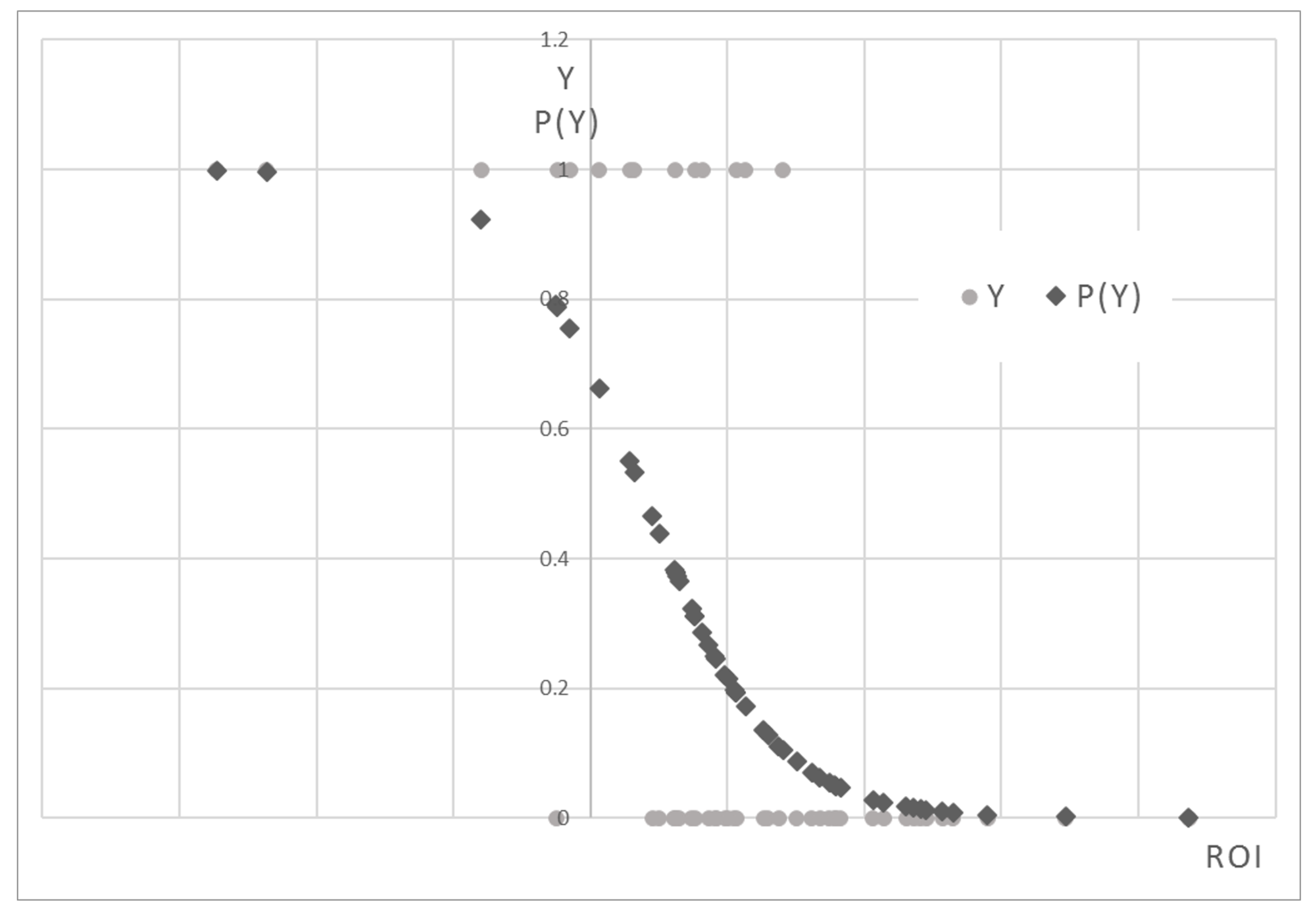
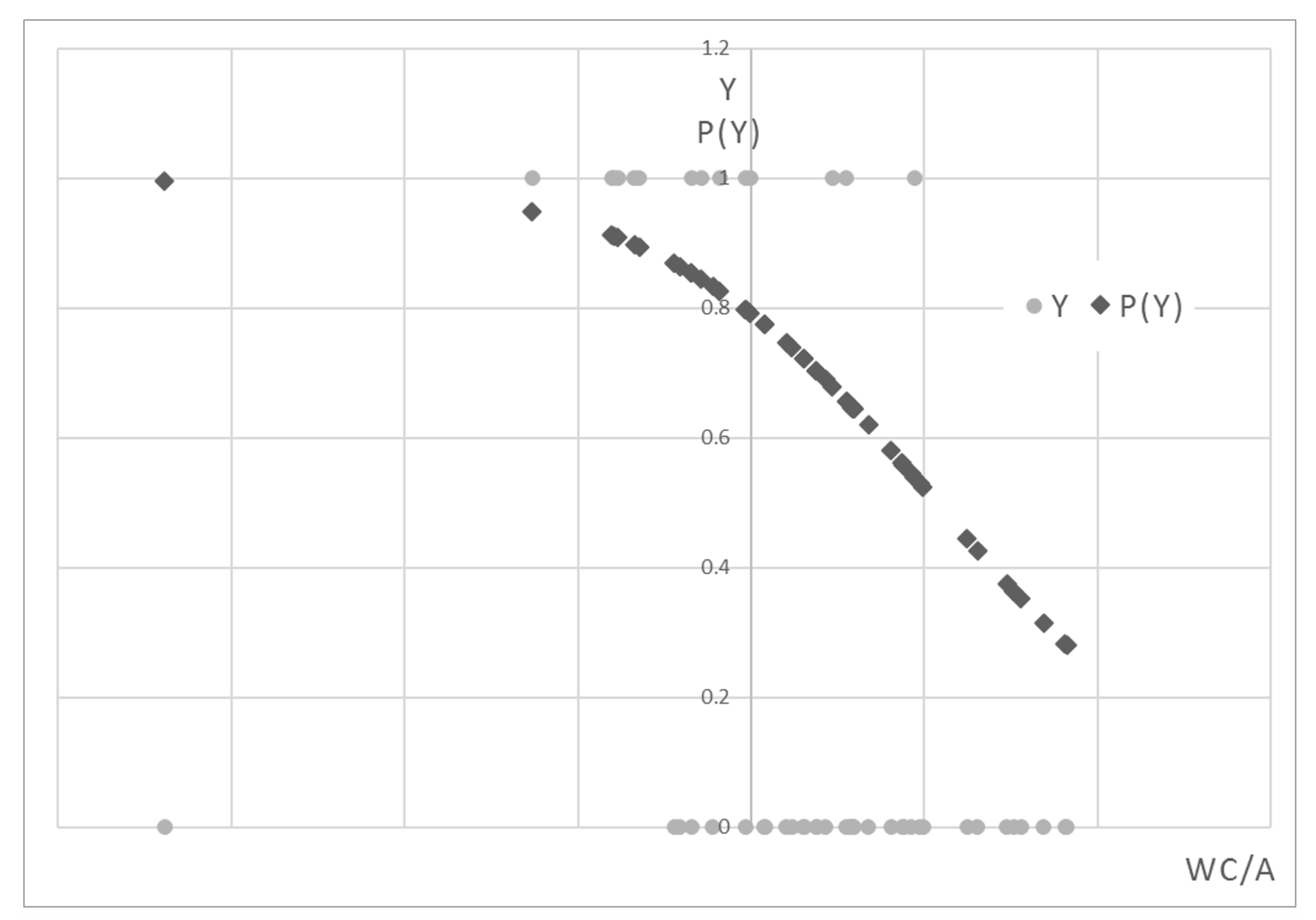
Figure 1 and Figure 2). Both the coefficients are negative showing that PD decreases with increasing covariates. As the Return on Investment (ROI) increases, the riskiness of the company decreases (Figure 1); as the Working Capital to Asset ratio increases (and, therefore, as the difference between current assets and current liabilities increases), the company becomes safer (Figure 2).
The points of the P(Y) constitute an inverse sigmoid: as the ROI increases, P(Y) decreases. They are concentrated mainly in the lower part of the graph, where P(Y) is less than 0.4. This is because in the sample there are more Type 0 firms than Type 1 ones. A probability function of this type is better suited to the observations, remaining within the constraints of 0 and 1.
This second inverse sigmoid has the same trend as the previous one. However, it is truncated, as no observation of the sample presents a probability as a function of the WC to asset ratio lower than 0.3.

4.2. Results for the LGD

Our dataset contains 55 defaulted loans, of which are known historical accounting movements, year of default, EAD, recovery time and presence of collateral (see Table A2). According to the definition, LGD is calculated as the complement to the one of the Recovery Rate (RR), the proportion of money financial institutions successfully collected minus the administration fees during the collection period, given the borrower has already defaulted Ye and Bellotti (2019):
L G D = 1 R R = 1 ( V R A C ) / E A D
where E A D is the exposure at default of each loan, A C stands for the administration costs incurred, discounted at the time of default, and V R is the present value of the recovered amount. Recovery time is standardized through the equation 1 e r t . The discount rate used is 10%. All data are shown in Appendix A. As in Hartmann-Wendels et al. (2014); Jones and Hensher (2004); Tsai (2013), and to avoid data separation that could be introduced by a finer partition of the dataset, we split the sample into three buckets so that the ‘ L G D * ’ column is categorized as (0, 1, 2) of each loan in relation to the L G D level. Therefore, the following rule applies:
Y i = 0 if L G D 30 % Y i = 1 if 30 % < L G D 70 % Y i = 2 if L G D > 70 % .
In the ‘COLLATERAL*’ column, the presence or absence of collateral is, respectively, indicated by 1 and 0.
At this point, the goal is to demonstrate in this sample how the presence of collateral and the length of the recovery time affects L G D . Loans with the lowest loss level are 15% of the sample; Category 1, where loss was between 30% and 70% of exposure, constituting 49% of total; loans with L G D greater than 0.7 are 36%. It is easy to understand that the average and the median of latent L G D are lower than 0.1 for the first category of loans, close to 0.5—and to the total average of the sample—for the second category, and almost 1 for the third. Moreover, only 17 credits of 55 were guaranteed by collateral (31%), 7 out of 8 in the first category, 6 out of 27 in the second one and 4 out of 20 in the third groups. Both mean and median of latent response variable are higher for loans without collateral than for the ones with collateral, confirming that collateral has positive effect on credit recovery. Both mean and median of recovery time grow as the L G D increases: as more time passes, it becomes more difficult to recover a loan. The first model shows the relationship between L G D trend and the presence of collateral. Estimating the model, it can be immediately noticed that this model does not fit very well to the data: Pearson’s chi-square corresponds to a small p-value that does not allow us to reject the null hypothesis according to which the model is good. Pseudo r-square is also very low and therefore unconvincing. The results are shown below (Table 10 and Table 11).
Certainly, a large part of this low fit score is attributable to the sample size, which is extremely small. However, the estimates of the model parameters are shown below (Table 12), which are still significant.
The second estimated model is the one that includes recovery time as regressor. Estimating the model, data fit measures are obtained first. The “Final” model has a better fit than the first one (Table 13).
LR Chi-Square test allows verifying if the predictor’s regression coefficient is not equal to zero. Test statistic is obtained from the difference between LR of Model 0 and LR of the final model. P-value (equal to 0.000—it represents the probability of obtaining this chi-square statistic (31.56) if in reality there is no effect of the predictive variables) compared with a specified alpha level—i.e., our willingness to accept a Type I error, which is generally set equal to 0.05—leads us to conclude that the regression coefficient of the model is not equal to 0. Pearson’s chi-square statistics and deviance-based chi-square statistics give us information on how suitable the model is for empirical observations. Null hypothesis is that the model is good; therefore, if p-value is large, then the null hypothesis is accepted, and the model is considered good. In this case, it is possible to say that the model is acceptable, as its results are satisfactory: it has a Pearson’s chi-square equal to 22.0, df = 19, p-value = 0.283; Deviance’s chi-square is equal to 23.5, df = 19, p-value = 0.218; the pseudo R-square measurements are also acceptable (Table 14), considering that the L G D is determined by many factors and recovery time is not the only feature.
In Table 15, it is possible to notice that recovery time is significant as well as directly proportional to L G D : the positive coefficient tells us that, as recovery time increases, L G D also increases, as expected. In fact, it is known from the literature that the best way to manage a bad credit is to act promptly and that, over time, the chances to recover a loan worsen.
The ‘threshold’ section contains estimates, in terms of logit, of cutoff points between categories of response variable. The value for [ L G D = 0 ] is the estimate of cutoff between the first and second class of L G D ; the value corresponding at [ L G D = 1 ] is the estimate of cutoff between the second and the third L G D classes. Basically, they represent points, in terms of logit, from which loans should be predicted in the upper class of L G D . For the purposes of this analysis, their interpretation is not particularly significant, nor is it useful to interpret these values individually. The only estimate of logit ordered regression coefficient that appears in the parameter estimates table is the one relating to the regressor. Conceptually, interpretation of this value is that when explanatory variable increases by one unit the level of the response variable is expected to change, according to its ordered log-odd regression coefficient. In our case, a unit time increment generates a variation of the ordered log-odd of being in a higher L G D category of 6.624. A corresponding p-value (0.000) that remains below the acceptance threshold of the null hypothesis ensures the significance of recovery time determining L G D . 
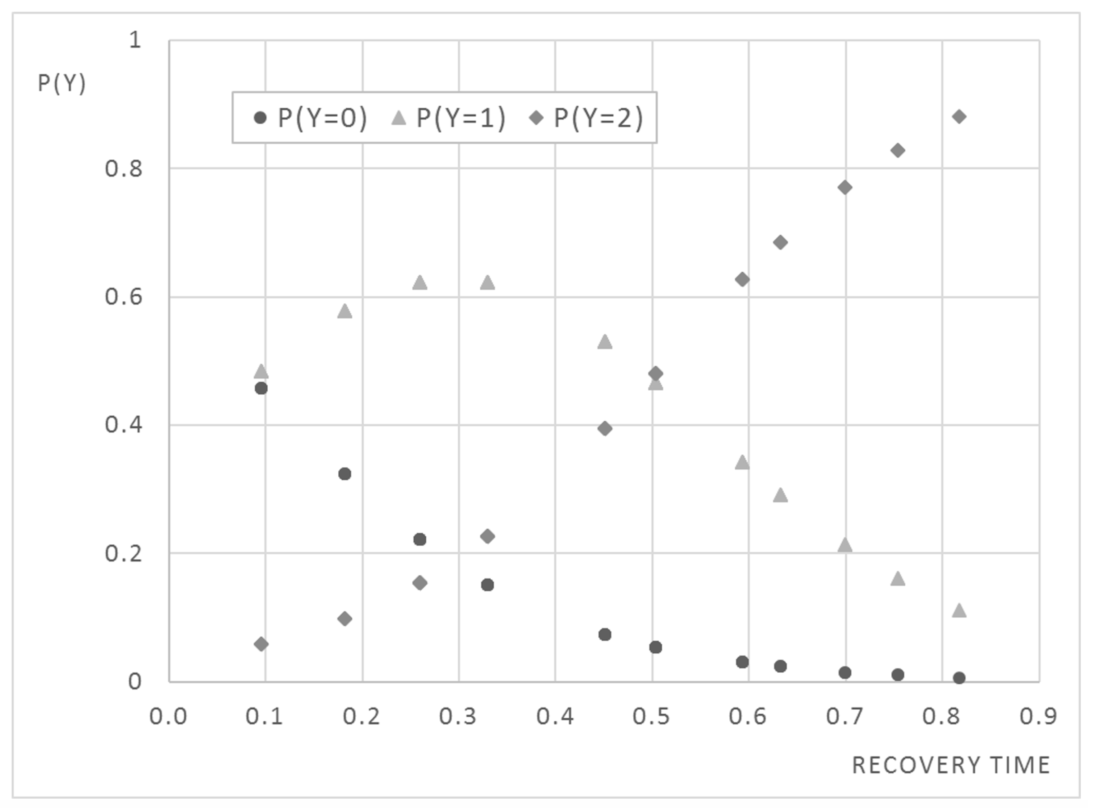
Figure 3 shows the probability curves of occurrence of each category related to recovery time.
Circles belong to probability curve that Y is equal to 0—the category with the lowest loss rate. Over time, this probability decreases until it is almost zero for loans, among the observed, with longest recovery times. Diamonds, instead, define the curve of probability that Y is equal to 2: here, loans have very high expected L G D , almost equal to one. This probability increases considerably over time. Finally, triangles outline the probability curve that Y is equal to 1, the class in which the expected L G D is between 0.30 and 0.70. It is increasing in the first part; starting from the moment in which the probabilities of the other two classes are equal and the respective curves intersect it starts to decrease till the end of time axis.

Poisson Estimation and Suitability Analysis

As mentioned, we divided the dataset into three groups as in Jones and Hensher (2004); Tsai (2013); Hartmann-Wendels et al. (2014). We found the ranges in Equation (8) to suit well our analysis but, in other contexts, it could be that these ranges are different. The logistic regression answers the question how many cases belong to a certain category. To assess the suitability of the classification, we ran a generalized linear model (GLM) Poisson regression. Table 16 and Table 17 provide the estimates for the models with (Model 1) or without the intercept (Model 2), respectively. The dispersion of the results is shown in Table 18. As illustrated, Model 2 (i.e., the model without intercept) performs better than Model 1 with little loss in terms of dispersion of residuals. Moreover, this analysis confirms that the most important factor is time.

5. Discussion

5.1. Logit Model in Risk

Applications of the logit model in the field of risk assessment have been numerous and still are, due to its simplicity as well as its effectiveness. However, over the years, although rather slowly compared to the evolution of corresponding literature Jones and Hensher (2004), there has been the development of innovative techniques regarding this approach, which have made it increasingly performed. Tsai (2013) overcame the usual failed–non failed dichotomy to also consider companies that are not bankrupt but that face slight financial distress events. He adopted the multinomial logit model in which the dependent variable assumes three different values, depending on whether the company is “not distressed”, “slightly distressed” or “in reorganization or bankruptcy”. For this purpose, within the covariates are included corporate governance factors (insiders’ ownership ratio, pledge of ownership ratio of the insiders, deviation ratio between voting and cash flow rights—where insiders include directors, supervisors, managers and large shareholders), in addition to the financial ratios (current assets to current liabilities, total liabilities to total assets, working capital to total assets, retained earnings to total assets, sales to total assets and net income to total assets) and market variables (market equity to total liabilities, abnormal returns, logarithm of the firm’s relative size, idiosyncratic standard deviation of each firm’s stock returns and logarithm of age). The idea stems from the assumption that many companies facing financial difficulties mask the accounting results to prevent their financial statements from showing losses recorded at the end of the year. The use of only financial ratios and market variables, in fact, would generate estimates polluted by such a lack of transparency of financial statements.
The investigation aims to evaluate whether the corporate governance variables are useful in order to reveal further information regarding the occurrence of slight distress events and, in general, whether the use of a model that includes these variables (CG model) better predicts PD compared to what a model based only on financial ratios and market variables (non-CG model) does Tsai (2013). Comparing the average of each covariate calculated for each group of companies, the results of the previous study are confirmed: in all financial ratios, the group of “not distressed” ranks first, with the best means; the “slightly distressed firms rank second and the “reorganized or bankrupt” ones are third. Unlike that study, however, in this case, all the financial variables are significant for the model, certainly due to the greater representativeness of the sample. Once the coefficients of the CG-model have been estimated, it results that, compared to the corporate governance variables, financial ratios are less relevant to the occurrence of slight distress events. This shows and confirms what was assumed at the beginning: managers of companies subject to slight financial difficulties tend to manipulate financial results. Conversely, financial ratios are more closely related to reorganization and bankruptcy events than corporate governance variables are. Although the CG model estimates show that market variables are significantly related to the occurrence of financial distress, it appears that they are more connected to reorganization and bankruptcy events than to slight distress ones; this is because reorganized and bankrupt firms show greater candor in divulging operational difficulties in their financial statements and investors can react in a timely fashion to their devaluation. Moreover, once the estimates of both models have been made and the respective probabilities that a company is in a group of three have been obtained, the accuracy tests show that, in general, the CG model outperforms the non-CG model.
According to Jones and Hensher (2004): “considering the case of firm failures, the main improvement is that mixed logit models include a number of additional parameters that capture observed and unobserved heterogeneity both within and between firms” that is the heterogeneity characterizing the behavior of subjects, i.e. the individual changes in tastes and preferences. In fact, while in the case of traditional logit model the influences deriving from behavioral heterogeneity flow incorrectly into the error term and the functional form of utility that each company q associates with each outcome i is given by
U i q = β q X i q + e i q
where X i q is the vector of observed characteristics of companies, β q is the parameter vector, e i q is the term of residuals, containing the effects not observed and it is assumed that the unobserved influences are distributed identically and independently among the alternative outcomes (therefore, it is possible to remove the subscript i from the term e), mixed logit model maximizes the use of behavioral information incorporated in the analyzed dataset through the partition of stochastic component e into two uncorrelated parts:
U i q = β q X i q + ( η i q + ϵ i q )
where η i q is the random term correlated with each alternative outcome, heteroscedastic and with generic density function f ( η i q | Ω ) ( Ω the fixed parameters of the distribution) and ϵ i q is the part i.i.d. over alternative outcomes and firms. For a given value of η i q , the conditional probability of each outcome i is the logit
L i ( η ) = exp ( β X i q + η i q ) j exp ( β X j q + η j q ) .
Since η is not given, the outcome probability is this logit formula integrated overall value of η weighted by the density of η :
P i = L i ( η ) f ( η | Ω ) d η .
hence the name “mixed”, indicating that the probability of an outcome i occurring is given by the mix of logits and f. Comparing the results of the analysis on financial distress events conducted by researchers, first with a standard logit model and then with the mixed logit model, the second is far better than the first.
Here, too, the dataset is made up of companies divided into three groups: non-failed firms, insolvent firms and firms which filed for bankruptcy. The independent variables are financial ratios (total debt to gross operating cash flow, working capital to total assets, net operating cash flow to total assets, total debt to total equity, cash flow cover and sales revenue to total assets). Both measures of goodness-of-fit and statistical tests provide indications on the best performance of mixed logit model. Results of the latter indicate that some variables have only one fixed parameter while others have up to three parameters, indicating the influence of behavioral heterogeneity not considered by other models. The multinomial logit model is rather poor in classifying financial distress firms: in its best performance, it predicts corporate default in 29% of cases. Conversely, mixed logit works very well in both cases of financial distress, even when one moves away from the reporting period: the accuracy rate in the five years following data collection drops to a minimum of 98.73% Jones and Hensher (2004).

5.2. Regressors

5.2.1. Regressors for the PD

Regarding the regressors, we aligned our analysis to the methodology available in literature. For example, on debt to equity, Achleitner et al. (2011), when evaluating value creation and pricing in buyouts, brought empirical evidence confirming that it is the “better proxy to account for the influence of leverage on equity returns”. On the same line, Penman et al. (2007) stated “net debt divided by the market value of equity is the generally accepted measure of leverage that captures financing risk” and Phongmekin and Jarumaneeroj (2018) affirmed that “according to the regression coefficients, a stock with higher value of third year’s net debt to equity ratio also has a high tendency for positive return”. The reason for that is quite straightforward as “the net debt would account for the available cushion and represent a more accurate measure of financial risk emanating from capital structure”. “An increasing net debt would put constraints on raising incremental capital and firms with high leverage would find it difficult and costly to access funds as compared to firms with less leverage” Nawazish et al. (2013). More in general, on the use of financial ratios, Tian and Yu (2017) found them useful as predictors in forecasting corporate default and Phongmekin and Jarumaneeroj (2018) found them useful to develop a predictive model about companies listed on the Stock Exchange of Thailand (SET).

5.2.2. Regressors for the LGD

Regressors for the L G D might be industry classification, size of loan, collateral, seniority of debts, product type, firm size, creditworthiness, firm age, macroeconomic condition, etc. “However, different studies suggest different factors and there is no consensus on these factors except collateral” Han and Jang (2013). This is in line with our findings as the only two relevant variables are collateral and recovery time.

6. Conclusions

On the classification model, a study made on similar dataset by Phongmekin and Jarumaneeroj (2018) has shown that classification techniques such as logistic regression (LR), decision tree (DT), linear discriminant analysis (LDA) and K-nearest neighbor (KNN), are comparatively good. In addition, they found that LR and LDA are “the most useful classifiers for risk averse investors—as both are not subject to uncertainty due to true positive counting bias”.
On the P D , we showed that the ROI and the WC to Asset are the most relevant variables. To check the quality of our results, we complemented the analysis by running the Firth’s penalized likelihood. The latter is a method of addressing issues of separability, small sample sizes and bias of the parameter estimates. Then, we demonstrated that the outcomes are similar.
On the L G D , several studies have certainly led to assertion that there are no universally valid models for any type of loans’ technical form Yashkir and Yashkir (2013). If a single solution has not yet been found on the issue of L G D modeling, it is because the loss rate depends on both external macroeconomic factors and individual characteristics of each credit institution. However, those who have tried to incorporate the effects of the economy by adding some macroeconomic variable to the model (see, for example, Bruche and González-Aguado (2010); Bellotti and Crook (2012); Leow et al. (2014)) did not report any significant improvement. For this reason, we share the opinion that L G D estimates should reflect the practice of each individual institution Dahlin and Storkitt (2014). Furthermore, the analysis carried out in this specific case shows how recovery time assumes great importance in determining the degree of loss, more than the presence of collateral to guarantee the credit. To maximize the recovery of a non-performing credit, the time taken to recover the credit should therefore be minimized. This is of great importance for Italy where bureaucracy is cumbersome, judicial system is slow and legal enforcement is inefficacy.

Author Contributions

Conceptualization, G.O. and R.P.; methodology, G.O.; software, G.O. and R.P.; validation, G.O. and R.P.; formal analysis, G.O.; investigation, G.O. and R.P.; resources, G.O. and R.P.; data curation, R.P.; writing—original draft preparation, G.O. and R.P.; writing—review and editing, G.O.; visualization, G.O. and R.P.; supervision, G.O.; and project administration, G.O. All authors have read and agreed to the published version of the manuscript.

Funding

This research received no external funding.

Conflicts of Interest

The authors declare no conflict of interest.

Appendix A. Dataset

Table A1. Dataset for PD’s estimate.
FirmNet Debt to Equity RatioY (dych.)Current RatioROIWorking Capital to Asset RatioDebt RatioAsset TurnoverROA
Aeffe0.1601.4540.1300.2930.8811.5030.073
Alkemy0.3001.3720.1060.2751.0491.4560.069
Autogrill0.9110.6960.106−0.1731.2533.5210.058
Basic Net0.4601.5280.1620.2920.7270.9230.125
B&C Speakers0.2002.6300.3470.8440.8061.9580.331
Bioera3.3710.721−0.237−0.3971.9542.994−0.295
Brembo0.1101.1380.2410.1020.9351.9200.173
Brunello Cucinello0.0501.8530.2300.4620.6831.8180.167
Campari0.3902.3520.1270.2960.8040.5690.098
Cairo Communication0.2600.7910.137−0.1110.9611.2990.101
Centrale del Latte Italia1.1610.9940.006−0.0031.0221.2790.003
Cellularline0.1303.0310.0860.4030.5390.5920.077
Class Editori2.5110.587−0.080−0.6321.6500.676−0.072
De Longhi0.2102.1080.2900.9061.2122.3840.212
Elica0.6900.9810.050−0.0141.1682.6270.013
Emak0.5701.9360.1050.4870.9211.3800.077
Enervit0.0401.2590.1680.1890.6962.4450.137
Fila1.3412.8470.0620.4721.0220.7440.013
Geox0.0901.617−0.0250.6541.0832.510−0.016
Giglio Group2.2810.758−0.024−0.3851.3571.2390.020
Immsi2.2510.6150.082−0.3371.3571.2390.020
I Grandi Viaggi0.3201.7320.0450.3380.8201.2240.027
Ivs0.9000.9510.076−0.0160.8380.7100.040
La Doria0.4701.6900.0980.4951.1071.9520.076
Landi Renzo0.8901.1620.1000.1181.2141.6610.040
Massimo Zanetti Beverage0.5501.3470.0740.1890.9771.7880.040
Marr0.4801.6540.2060.6232.0983.4080.140
Mondadori0.8901.1620.1750.1521.2272.504−0.492
Monrif1.2710.5610.029−0.4021.3531.8270.107
Netweek1.0910.802−0.273−0.3232.3192.361−0.455
Newflat Food0.2201.1280.2140.2902.8445.0190.098
Orsero0.2401.5210.0610.4361.3504.8910.041
OVS0.4301.0870.0920.0400.9131.2710.004
Piaggio1.1010.8740.113−0.0911.3841.7430.042
Pininfarina0.0801.5770.0650.2850.9031.7180.035
Piquadro0.0901.8270.1790.7571.2872.1540.104
Pirelli0.7001.1020.0910.0371.0760.7140.056
Poligrafici Editore0.7600.8080.062−0.1731.3841.988−1.612
Ratti0.0402.2600.2650.9121.3711.9860.187
Rcs0.7400.7200.257−0.2221.3102.0770.178
Reno De’ Medici0.3401.2440.1500.1531.00522.0800.092
Rosss2.3211.126−0.0150.2752.8443.912−0.040
Salvatore Ferragamo0.2202.6330.2450.7780.6532.1790.145
Sanlorenzo0.2101.2800.1780.4402.0712.8720.096
Sogefi1.2410.8520.141−0.1441.9383.3860.036
Technogym0.1701.1850.4370.2151.6002.5560.378
Tod’s0.0701.8700.0630.2950.4780.8230.040
Triboo0.1700.8490.076−0.2061.6851.5580.050
Unieuro0.0600.7340.236−1.6927.6832.0260.118
Valsoia0.3203.0060.1820.7380.5651.8220.219
Vianini1.4813.0280.0320.2340.6540.0920.011
Table A2. Dataset for LGD’s estimate.
Loan IDLGDLGD *Recov. TimeCollateralCollateral *
1010%00.095yes1
1020%00.095yes1
10389%20.698no0
10470%20.593yes1
10645%10.753no0
10785%20.753no0
11119%00.095no0
11286%20.698no0
11445%10.632yes1
1159%00.181yes1
11692%20.632no0
11980%20.632no0
12229%00.451yes1
12391%20.503no0
12471%20.503no0
12590%20.503no0
12764%10.503yes1
12816%00.259yes1
13063%10.593no0
13168%10.593no0
13387%20.451no0
13494%20.451no0
13590%20.451no0
13744%10.593yes1
13894%20.817yes1
1400%00.593yes1
14193%20.503no0
14240%10.503no0
144100%20.503yes1
14535%10.451yes1
14697%20.451no0
14861%10.451no0
15057%10.503no0
15160%10.329no0
15239%10.329yes1
15353%10.329no0
15594%20.329no0
15639%10.329no0
15846%10.329yes1
15957%10.329no0
16056%10.329no0
16155%10.259no0
16256%10.259no0
16358%10.259no0
16497%20.259yes1
16592%20.259no0
16692%20.259no0
16755%10.259no0
16855%10.259no0
16955%10.259no0
17049%10.181no0
17151%10.181no0
17253%10.181no0
17354%10.259no0
1740%00.095yes1
* Variables expressed in categories for the purpose of the analysis.

References

  1. Achleitner, Ann-Kristin, Reiner Braun, and Nico Engel. 2011. Value creation and pricing in buyouts: Empirical evidence from Europe and North America. Review of Financial Economics 20: 146–61. [Google Scholar] [CrossRef]
  2. Andrews, Dan, and Federico Cingano. 2014. Public policy and resource allocation: Evidence from firms in OECD countries. Economic Policy 29: 253–96. [Google Scholar] [CrossRef]
  3. Andrews, Dan, Chiara Criscuolo, and Peter N. Gal. 2015. Frontier Firms, Technology Diffusion and Public Policy: Micro Evidence from OECD Countries. Paris: OECD iLibrary. [Google Scholar]
  4. Arnold, Jens Matthias, Giuseppe Nicoletti, and Stefano Scarpetta. 2011. Does Anti-Competitive Regulation Matter for Productivity? Evidence from European Firms. Amsterdam: Elsevier. [Google Scholar]
  5. Barone, Guglielmo, and Federico Cingano. 2011. Service regulation and growth: Evidence from OECD countries. The Economic Journal 121: 931–57. [Google Scholar] [CrossRef]
  6. Barrios, Salvador, and Jean-Claude Burgelman. 2008. Europe needs more Lisbon to make the ICT investments effective. Intereconomics 43: 124–34. [Google Scholar] [CrossRef] [Green Version]
  7. Bartelsman, Eric, John Haltiwanger, and Stefano Scarpetta. 2009. Measuring and analyzing cross-country differences in firm dynamics. In Producer Dynamics: New Evidence from Micro Data. Chicago: University of Chicago Press, pp. 15–76. [Google Scholar]
  8. Bellotti, Tony, and Jonathan Crook. 2012. Loss given default models incorporating macroeconomic variables for credit cards. International Journal of Forecasting 28: 171–82. [Google Scholar] [CrossRef] [Green Version]
  9. Bentivogli, Chiara. 2009. Taxi regulation and the Bersani reform: A survey of major Italian cities. European Transport 41: 1–27. [Google Scholar]
  10. Bravo-Biosca, Albert, Chiara Criscuolo, and Carlo Menon. 2016. What drives the dynamics of business growth? Economic Policy 31: 703–42. [Google Scholar] [CrossRef]
  11. Bruche, Max, and Carlos González-Aguado. 2010. Recovery rates, default probabilities, and the credit cycle. Journal of Banking & Finance 34: 754–64. [Google Scholar]
  12. Bugamelli, Matteo, Francesca Lotti, Monica Amici, Emanuela Ciapanna, Fabrizio Colonna, Francesco D’Amuri, Silvia Giacomelli, Andrea Linarello, Francesco Manaresi, and Giuliana Palumbo. 2018. Productivity Growth in Italy: A Tale of a Slow-Motion Change. Bank of Italy occasional paper. Amsterdam: Elsevier. [Google Scholar]
  13. Chiarini, Bruno. 1999. The composition of union membership: The role of pensioners in Italy. British Journal of Industrial Relations 37: 577–600. [Google Scholar] [CrossRef]
  14. Cramer, Jan Salomon. 2003. Logit Models from Economics and Other Fields. Cambridge: Cambridge University Press. [Google Scholar]
  15. Dahlin, Fredrik, and Samuel Storkitt. 2014. Estimation of Loss Given Default for Low Default Portfolios. Technical Report. Available online: https://www.math.kth.se/matstat/seminarier/reports/M-exjobb14/140512.pdf (accessed on 2 September 2020).
  16. De Luca, Davide Maria. 2017. I Sindacati in Mano a chi Non Lavora. Available online: https://www.ilpost.it/2017/07/29/sindacati-pensionati/ (accessed on 2 September 2020).
  17. European Banking Authority (EBA). 2017. Draft Implementing Standards Amending Implementing Regulation (EU) No 680/2014. Paris: EBA. [Google Scholar]
  18. Fabbri, Daniela. 2010. Law enforcement and firm financing: Theory and evidence. Journal of the European Economic Association 8: 776–816. [Google Scholar] [CrossRef]
  19. Firth, David. 1993. Bias reduction of maximum likelihood estimates. Biometrika 80: 27–38. [Google Scholar] [CrossRef]
  20. Fucci, Frederick, and Francesco Fucci. 1999. Bersani decree opens Italian energy market. International Financial Law Review 18: 27. [Google Scholar]
  21. Gim, Tae-Hyoung Tommy, and Joonho Ko. 2017. Maximum likelihood and Firth logistic regression of the pedestrian route choice. International Regional Science Review 40: 616–37. [Google Scholar] [CrossRef]
  22. Han, Chulwoo, and Youngmin Jang. 2013. Effects of debt collection practices on loss given default. Journal of Banking & Finance 37: 21–31. [Google Scholar]
  23. Hartmann-Wendels, Thomas, Patrick Miller, and Eugen Töws. 2014. Loss given default for leasing: Parametric and nonparametric estimations. Journal of Banking & Finance 40: 364–75. [Google Scholar]
  24. Heinze, Georg, and Michael Schemper. 2002. A solution to the problem of separation in logistic regression. Statistics in Medicine 21: 2409–19. [Google Scholar] [CrossRef]
  25. Istat. 2020. La Protezione Sociale in Italia e in Europa. Available online: https://www.istat.it/it/archivio/241933 (accessed on 2 September 2020).
  26. Jappelli, Tullio, Marco Pagano, and Magda Bianco. 2005. Courts and banks: Effects of judicial enforcement on credit markets. Journal of Money, Credit and Banking 37: 223–44. [Google Scholar] [CrossRef] [Green Version]
  27. Jones, Stewart, and David A Hensher. 2004. Predicting firm financial distress: A mixed logit model. The Accounting Review 79: 1011–38. [Google Scholar] [CrossRef]
  28. Laeven, Luc, and Christopher Woodruff. 2004. The Quality of the Legal System, Firm Ownership, and Firm Size. Washington, DC: The World Bank. [Google Scholar]
  29. Leow, Mindy, Christophe Mues, and Lyn Thomas. 2014. The economy and loss given default: Evidence from two UK retail lending data sets. Journal of the Operational Research Society 65: 363–75. [Google Scholar] [CrossRef]
  30. Moscatelli, Mirko, Fabio Parlapiano, Simone Narizzano, and Gianluca Viggiano. 2020. Corporate default forecasting with machine learning. Expert Systems with Applications 161: 113567. [Google Scholar] [CrossRef]
  31. Muroni. 2019. Gli Stabilimenti Balneari, il Governo fa Danni Anche alle Spiagge. Available online: https://www.linkiesta.it/2019/05/concessioni-stabilimenti-balneari-procedura-infrazione-ue-italia/ (accessed on 2 August 2020).
  32. Nawazish, Mirza, Mawal Sara Saeed, and Kumail Abbas Rizvi. 2013. The pricing of size, book to market and financial leverage in Euro stocks. Economic Research-Ekonomska Istraživanja 26: 177–90. [Google Scholar]
  33. Orlando, Giuseppe, and Maximilian Haertel. 2014. A parametric approach to counterparty and credit risk. Journal of Credit Risk 10: 97–133. [Google Scholar]
  34. Panzani, Luciano. 2012. Il Fallimento e le Altre Procedure Concorsuali. 3 vols. Torino: UTET Giuridica. [Google Scholar]
  35. Penman, Stephen H, Scott A Richardson, and Irem Tuna. 2007. The book-to-price effect in stock returns: Accounting for leverage. Journal of Accounting Research 45: 427–67. [Google Scholar] [CrossRef]
  36. Phongmekin, Athit, and Pisit Jarumaneeroj. 2018. Classification models for stock’s performance prediction: A case study of finance sector in the stock exchange of Thailand. Paper presented at 2018 International Conference on Engineering, Applied Sciences, and Technology (ICEAST), Phuket, Thailand, July 4–7; pp. 1–4. [Google Scholar]
  37. Rajan, Raghuram G, and Luigi Zingales. 2004. Saving Capitalism from the Capitalists: Unleashing the Power of Financial Markets to Create Wealth and Spread Opportunity. Princeton: Princeton University Press. [Google Scholar]
  38. Rajan, Raghuram G, Luigi Zingales, and Krishna B Kumar. 2001. What Determines Firm Size? Amsterdam: Elsevier. [Google Scholar]
  39. Sanders, Mark, Mikael Stenkula, Luca Grilli, Andrea M Herrmann, Gresa Latifi, Balázs Páger, László Szerb, and Elisa Terragno Bogliaccini. 2020. A reform strategy for Italy. In The Entrepreneurial Society. Berlin/Heidelberg: Springer, pp. 127–62. [Google Scholar]
  40. Sandulli, M., and G D’Attorre. 2016. La Nuova Mini-Riforma Della Legge Fallimentare. Torino: G. Giappichelli Editore. [Google Scholar]
  41. Tian, Shaonan, and Yan Yu. 2017. Financial ratios and bankruptcy predictions: An international evidence. International Review of Economics & Finance 51: 510–26. [Google Scholar]
  42. Tsai, Bi-Huei. 2013. An early warning system of financial distress using multinomial logit models and a bootstrapping approach. Emerging Markets Finance and Trade 49: 43–69. [Google Scholar] [CrossRef]
  43. Van Reenen, John, Nicholas Bloom, Mirko Draca, Tobias Kretschmer, Raffaella Sadun, Henry Overman, and Mark Schankerman. 2010. The Economic Impact of ICT. Final report. London: London School of Economics, Centre for Economic Performance, pp. 1–217. [Google Scholar]
  44. Violati, F. 2001. Italian electric systems before and after the law reform. Energia (Roma) 22: 30–46. [Google Scholar]
  45. Wang, Xuefeng. 2014. Firth logistic regression for rare variant association tests. Frontiers in Genetics 5: 187. [Google Scholar] [CrossRef] [Green Version]
  46. Yashkir, Olga, and Yuriy Yashkir. 2013. Loss given default modelling: Comparative analysis. Journal of Risk Model Validation 7: 1. [Google Scholar] [CrossRef] [Green Version]
  47. Ye, Hui, and Anthony Bellotti. 2019. Modelling recovery rates for non-performing loans. Risks 7: 19. [Google Scholar] [CrossRef] [Green Version]
Figure 1. PD as the ROI changes.
Ijfs 08 00068 g001
Figure 2. PD as the WC/A changes.
Ijfs 08 00068 g002
Figure 3. Probability of occurrence of each category for recovery time.
Ijfs 08 00068 g003
Table 1. Descriptive statistics for Net-Debt-to-Equity ratio.
FrequencyMeanMedianStd. Dev.
Healthy370.3280.2400.249
Risky141.6561.3020.749
Total510.6920.4340.741
Table 2. Descriptive statistics for covariates.
Current RatioROIWC to AssetDebt RatioAsset TurnoverROA
HealthyMean1.5580.1540.2721.3011.9910.046
Median1.4540.1370.2921.0521.9520.092
S.D0.6110.0940.4501.1770.9600.308
RiskyMean1.1010.001−0.1371.5541.850−0.059
Median0.8270.030−0.1591.3701.5780.012
S.D0.7950.1240.3080.6221.2050.167
TotalMean1.4320.1120.1601.3701.9520.017
Median1.2440.1050.2151.1071.8270.058
S.D0.6890.1230.4521.0541.0220.279
Table 3. Model 1 parameter estimates.
Coef.S.E.Walddfp-Value
Current Ratio1.4241.2171.37110.242
ROI−4.45413.2976.71310.010
WC to Asset−8.33443.6615.18310.023
Debt Ratio−1.4230.8422.85510.091
Asset Turnover0.7790.6161.59610.207
ROA2.3872.6080.83810.360
Constant1.0562.0260.27210.002
Table 4. Model 2 parameter estimates.
Coef.S.E.Walddfp-Value
ROI−26.6429.887.27110.007
WC to Asset−2.7821.2035.34810.021
Constant1.4530.8912.66310.003
Table 5. Model 2 parameter estimates with Firth PLR.
Coef.S.E.Lower 0.95Upper 0.95Chi-Sq.p-Value
ROI−22.318.413−44.009−8.29015.5098.21 × 10 5
WC to Asset−2.3721.0806−4.767−0.4635.7730.016
Constant1.1550.798−0.2803.0472.3670.124
Table 6. Goodness of fit for the logistic regression (ML estimates).
−2 Log-LikelihoodCox–Snell R SquareNagelkerke R Square
32.9710.4110.594
Table 7. Goodness of fit for the logistic regression (Firth PLR estimates).
−2 Log-Likelihoodp-ValueWald Testp-Value
23.3788.39 × 10 6 7.8890.019
Table 8. Contingency table for Hosmer–Lemeshow test.
HealthyRisky
ObservedExpectedObservedExpectedTotal
154.99900.0015
254.98000.0205
354.92300.0775
454.74300.2575
544.43810.5625
633.98121.0195
743.67811.3225
832.84222.1585
932.01522.9855
1000.40165.5996
Table 9. Percentage correctly predicted by Model 2.
Predicted
HealthyRiskyCorrect Percentage
ObservedHealthy34391.9
Risky6857.1
Overall Percentage 82.4
Table 10. Model 1 goodness of fit.
Chi-Squaredfp-Value
Pearson5.11110.024
Deviance5.34310.021
Table 11. Model 1 pseudo R-square.
Cox–SnellNagelkerkeMcFadden
0.1360.1570.073
Table 12. Model 1 parameter estimates.
EstimateS.E.Walddfp-Value
Threshold[LGD=0]−0.7200.4882.17710.140
[LGD=1]1.9410.58311.07910.001
Location[COLL=0]1.7480.6287.74210.005
[COLL=1]0 *..0.
* The parameter is set to zero because it is redundant.
Table 13. Model 2 measures of fit.
Model−2 Log-LikelihoodChi-Squaredfp-Value
Intercept Only61.495
Final44.72916.77510.000
Table 14. Pseudo R-square of Model 2.
Cox–SnellNagelkerkeMcFadden
0.2630.3040.153
Table 15. Model 2 parameter estimates.
EstimateS.E.Walddfp-Value
Threshold[LGD=0]0.4630.6740.47210.492
[LGD=1]3.4120.84716.23710.000
LocationRECOV. TIME6.6241.78513.76810.000
Table 16. GLM Poisson Model 1 parameter estimates.
Coef.Std. Errorz Valuep-Value
Time1.53520.66502.3090.0210
Collateral−0.52550.3005−1.7490.0804
Constant−0.33270.3337−0.9970.3187
Table 17. GLM Poisson Model 2 parameter estimates.
Coef.Std. Errorz Valuep-Value
Time0.9220.2763.3390.001
Collateral−0.5810.294−1.9780.048
Table 18. GLM Poisson estimate: dispersion analysis.
Deviance of the Residuals
Min1QMedian3QMax
Pois. mod. 1−1.452−0.286−0.0660.3431.370
Pois. mod. 2−1.478−0.383−0.1720.3121.249
Publisher’s Note: MDPI stays neutral with regard to jurisdictional claims in published maps and institutional affiliations.

