A Study on the Pass-Through Rate of the Exchange Rate on the Liquid Natural Gas (LNG) Import Price in China


Graduate School of Humanities and Social Sciences, Saitama University, 255 Shimo-Okubo, Sakura-ku, Saitama 338-8570, Japan
*
Author to whom correspondence should be addressed.
Int. J. Financial Stud. 2020, 8(4), 70; https://0-doi-org.brum.beds.ac.uk/10.3390/ijfs8040070
Submission received: 21 October 2020
/
Revised: 6 November 2020
/
Accepted: 9 November 2020
/
Published: 16 November 2020
Abstract
:The Chinese liquid natural gas (LNG) import price has been unstable because the stability of LNG import prices is related to changes in the exchange rates. This paper analyzes the pass-through rate of the Chinese Yuan (CNY) and Japanese Yen (JPY) on the Chinese LNG import price. The Time-Varying Parameter vector autoregressive (TVP-VAR) model is adopted to verify the pass-through rate of the exchange rates on the LNG import price using the Markov chain Monte Carlo (MCMC) method. Since September 2005, the JPY pass-through rate on the Chinese LNG import price has been decreasing while that of the CNY has been increasing. Notably, the pass-through rate of CNY began to exceed that of JPY after 2008. Moreover, since 2005, the lag effect of the CNY on the Chinese LNG import price became longer compared to JPY. If any new currency reform of the CNY is implemented in the future, then the impact of JPY on the Chinese LNG import price could be reduced and the lag effect of the CNY on the Chinese LNG import price could become longer. Therefore, the fluctuation of the CNY is becoming an important factor in understanding the movements of the Chinese LNG import price. This implies the significance of considering the effect of the exchange rate on an energy market when the market is influenced by a monetary reform of the importing country.
1. Introduction
North America, West Europe, and Asia-Pacific are the main markets for natural gas consumption in the world but in all of these regions, the liquid natural gas (LNG) import price has been unstable. For example, according to British Petroleum (BP) (2014, 2015), the Japanese LNG import price in Asia-Pacific regions decreased 57.5% from $16.33 to $6.94, the US Natural gas import price declined 43.33% from $4.35 to $2.46, and the UK Heren NBP Index of natural gas import price depreciated 43.15% from $8.25 to $4.69 during 2014–2016. Comparing the changes in the LNG import prices among Japan, the US, and the UK, it is noticeable in this example that the Japanese LNG import price is higher compared to the US and UK markets. The Japanese LNG price and the LNG import price in the Asian area have been fluctuating greatly at a higher price level (Ministry of Economy 2015).
One reason why the Asian LNG price has been higher than other regions is that the Asian LNG import price is known to be related to the average price of Japanese CIF (Cost, Insurance, and Freight) crude oil import price (Ministry of Economy 2016). The CIF crude oil has been kept at a higher price to protect sellers and buyers involved in the crude oil trade (Kawamoto and Tsuzaki 2007), and as the international crude oil price increases, the CIF price increases accordingly, making the LNG import price higher. Furthermore, the Asian LNG import price has been much higher than that of Western countries due to the Asian premium, which is a premium imposed on Asian countries’ LNG imports from the major gas producers. From the perspective of price stability, it is necessary to reconstruct a different pricing mechanism from the conventional one, which reflects the supply-demand balance on the Asian LNG import price. This is crucial for the Asian natural gas markets to attract market participants (Tong et al. 2014; Choi and Heo 2017). However, little is known about how the market mechanism functions in determining LNG import prices in the Asian region.
With the development of the Chinese economy, the demand for energy (especially natural gas) has increased dramatically. Since 1978, environmental problems such as PM 2.5 have intensified in China. To cope with such environmental problems, the Chinese government, proposed by the National Development and Reform Commission, announced a decision to change the supply and demand structure from fossil fuels to green energy between 2016–2020 (National Energy Board (NEB) 2016) under the Paris agreement on 3 September 2016. However, according to British Petroleum (BP) (2019), the Chinese consumption of natural gas increased substantially from 81.9 in 2008 to 283 billion cubic meters in 2018, and the Chinese domestic production of natural gas increased from 80.9 to 161.5 billion cubic meters between 2008 and 2018.
Furthermore, factors such as the risk of drastic changes in foreign exchange rates will affect the development of East Asian benchmark prices for the LNG spot market (Shi and Hari 2016). The above mentioned Asian premium issue and the risks from the foreign exchange rate changes are likely to become more serious as China continues to enhance more LNG imports through the spot market in the future. To address this situation, it is necessary to stabilize LNG import prices. Additionally, the Chinese government should re-examine factors such as foreign exchange risks that play an important role in determining the LNG import benchmark prices. This is crucial since the LNG import benchmark price reflects the supply-demand balance in a real-time way, and it is influential for ensuring the economic efficiency and stability of a natural gas supply. Furthermore, stabilizing the LNG import price in China is imperative for establishing a stable benchmark price and improving its energy security and pricing power for natural gas in the Asia-Pacific markets (Tong et al. 2014).
Another aspect we need to be aware of when investigating the effects of the exchange rate on the Chinese LNG import price is the Chinese Yuan’s (CNY) monetary reform. Since July 2005, China has made changes to the CNY exchange rate against the US dollar. However, when China began to apply this monetary reform in 2005, the daily fluctuation of CNY against the US dollar became less than 0.3%. According to the International Monetary Fund (IMF), until 2015, China had a crawling-peg arrangement for its exchange rate regime. On 11 August 2015, the People’s Bank of China (PBC) took a decisive step towards floating the CNY. With China’s large economic scale and the increasing use of the CNY, the CNY was included in the Special Drawing Right (SDR) basket of the International Monetary Fund (IMF) in 2016. Thus, from November 2016, China introduced a monetary system to peg the CNY against the basket of currencies. Liu and Chen (2017) reported that a more flexible exchange rate regime will bring about a stronger transmission effect from the exchange rate and can cause inflation in China. Since the 2016 monetary reform, there is a debate about whether changes in the CNY’s value have effects on the prices of imported goods.
However, up until now, no studies have investigated the exchange rate pass-through of CNY on the Chinese LNG import price considering the effects of CNY monetary reform. To bridge this gap, this study identifies the level of the pass-through rate of the exchange rate on LNG import price. The exchange-rate pass-through refers to the ratio of the price of traded goods that changes with the exchange rate (John et al. 1992).
This research has the following two objectives. First, the study analyzes how the CNY and JPY influence the Chinese LNG import price. The import price of LNG in China is linked with the Japan Crude Cocktail (JCC) price (Martono and Aruga 2018), and the import benchmark price of LNG is likely connected to the Japanese Yen (JPY). Hence, the study considers the effects of the foreign exchange risk on the Chinese LNG import price by comparing the influences on the LNG import price between CNY and JPY. Second, we examine the levels and the length of the pass-through rate of these currencies on the Chinese LNG import price. We do this because it is still not clear to what extent the exchange rate fluctuations influence the Chinese LNG import prices compared to JPY after the 2005 CNY monetary reform.
We expect that before the monetary reform, JPY will have more influence on the LNG price compared to CNY, but this effect will become smaller after the 2005 monetary reform. This is because a study finds that countries with higher exchange rate volatilities have higher pass-through elasticities on import prices (Jose and Goldberg 2006) and it is known that the volatility of JPY has been higher compared to CNY before 2005. It is also believed that the pass-through rate of JPY on LNG import price will become smaller and shorter after the monetary reform, while that of the CNY will become larger and longer. We expect this result since as the volatility of the CNY increases, the exchange rate risk in the LNG trading market has been gradually transferred to the CNY after 2005, and the effects from the CNY will become more significant in the Chinese LNG market.
The contributions of the present paper are the following. First, from the perspective of discovering the Chinese LNG import price, suppliers in the international LNG market need to consider the impact of exchange rate fluctuations on the Chinese LNG import price. Therefore, the results of this study provide valuable price discovery information for the international LNG suppliers exporting LNG to China. Second, the paper could be a good reference to energy-consuming countries that need to mitigate the effects of exchange rate changes on energy prices. As China is a country whose exchange rate rule is changing rapidly, the current study could be a useful source for understanding the impact of monetary reform on energy markets. Finally, this is one of the first studies to apply the Time-Varying Parameter vector autoregressive (TVP-VAR) model on an energy market to consider the effects of dynamic changes in the estimated parameters. Application of the TVP-VAR model is becoming popular in monetary and economic studies, but this method has not been used often for analyzing the dynamics of energy markets. Hence, the study can help scholars involved in analyzing energy markets with dynamic changes to understand the effectiveness of applying the TVP-VAR model on energy market data.
2. Previous Studies
Many studies have analyzed the pass-through rate of exchange rate on the import and export commodity prices. Some studies concluded that exchange rates have an incomplete pass-through on import commodity prices (Shinkai 2011; Choudhria and Hakura 2015; Pennings 2017) but Choudhria and Hakura (2015) showed that the pass-through from the exchange rate to import and export goods are different. They revealed that there is an incomplete pass-through from the exchange rate to import goods but there is a significant pass-through on the export goods. Pennings (2017) indicated that the pass-through is incomplete for producer prices. Furthermore, Kurtović et al. (2018) found that the pass-through rate on import and export goods are asymmetric in the cases of monetary appreciation and depreciation.
Moreover, according to Ceglowski (2010), in addition to oil prices, most of the pass-through rate on the US import goods dropped sharply from 1992 to 2006 (Sekine 2006), and the same conclusion was reported in Japan after 1970 (Sekine 2006; Shioji and Uchino 2009). Shinkai (2011) found that the pass-through rate on import price increases when exchange rate volatility increases in the short run, but this trend is associated with inflation in the long run. Sasaki (2019) found that Japan’s import pass-through rate had been declining, but it started to increase during the financial crisis. On the other hand, Kurtović et al. (2018) reported that there has been no decrease in the pass-through rates on the aggregate import prices of 7 Southeast European countries. Hui et al. (2013) reported that compared to developed countries, developing countries have a higher pass-through rate. Thus, it is likely that the pass-through rate on the Chinese LNG import price will be high, but up until now, no studies have confirmed the extent of the pass-through rate on the Chinese LNG import price.
We would also like to introduce studies related to the recent development of the methods used for analyzing the pass-through rate on import prices. Conventionally, the Vector autoregression (VAR) model has been applied for investigating the pass-through rate on commodity prices (Marazzi et al. 2005; Shinkai 2011). However, recently, according to the idea that the economic structure and conditions of financial policy change over time, the pass-through rate on import commodity prices was analyzed by considering the effects of changes in the estimated parameters over time (Sasaki 2019). For example, Primiceri (2005) applied the time-varying parameter VAR (TVP-VAR) model to investigate the effects of changes in the US monetary policy in the 1970s and early 1980s. Nakajima and Watanabe (2012) developed the TVP-VAR extrapolation program in OX software using the macro data of Japan. They suggested that compared to VAR model fixing parameters, TVP-VAR considering time-varying parameters improves the accuracy of the prediction of any variable (Nakajima and Watanabe 2012). Studies such as Shioji and Uchino (2009) and Shioji (2010) also measured the pass-through rate of the exchange rate on various commodities using the TVP-VAR.
Finally, there are a lot of concerns about how the fluctuations of the CNY will influence the Chinese economy, production, and import and export prices over time. However, there is no study investigating how the Chinese LNG import price have been and will be affected by the CNY and JPY fluctuations in the aftermath of China’s currency reform process. To cover this gap, this study examines the influence of the JPY and CNY on the Chinese LNG import price and compares the pass-through rate of these currencies on the Chinese LNG import price using the latest data available.
Our study is also novel in the sense that although most previous studies analyzed the pass-through rate by using the VAR model, the current study uses the TVP-VAR model to estimate the effects of the monetary rates on the Chinese LNG import price. This model enables us to consider the effects of dynamic changes in the estimated parameters.
3. Materials and Methods
The pass-through rate of the exchange rate on the Chinese LNG import price was estimated using four variables: the CNY (), JPY (), Chinese LNG import price (), and Japanese crude oil price (). Since Asian LNG import price is linked with the JCC crude oil price (Martono and Aruga 2018) and causes major impacts on the global natural gas industry chain, the Japanese crude oil price was included in the study.
Our econometric model was based on Primiceri’s TVP-VAR model (Nakajima and Watanabe 2012), which incorporates the effects of changes in the parameters during the test period. The model was estimated by using the Monte Carlo experiment with the OX 6 Console. Before estimating the TVP-VAR model, we tested the stationarity of our test variables with unit root tests. Then, we tested the cointegration between our variables to see if the VAR model was a suitable model for applying the data.
3.1. Unit Root and Cointegration Test Method
To identify the stationarity of our test variables, we applied the Augmented Dickey–Fuller (ADF), Phillips–Perron (PP), and Kwiatkowski–Phillips–Schmidt–Shin (KPSS) tests. The ADF and PP test the non-stationarity of the variables while the KPSS tests the stationarity of the variables.
After the order of integration was confirmed with the unit root tests, we performed the Johansen cointegration tests. The Johansen tests were conducted using the two monetary rates and LNG and crude oil prices: and . Eviews 8.0 software was used for this purpose.
3.2. TVR-VAR Model
Based on the assumption that the variables have unit roots and are not cointegrated, the TVP-VAR model has a different structure from the VAR model; the estimated parameters change over time (Primiceri 2005). To consider such parameter changes over time, we applied the TVP-VAR model on the CNY (E1), JPY (E2), Chinese LNG average import price (PL), and JCC average crude oil price. The JCC price was included in our model, which was mainly to avoid the impact of the JCC price on foreign exchange and to better understand the impact of the exchange rate on the Chinese LNG import price. The lag order of the time-varying model was determined by using the minimum AIC value obtained from the VAR model. In this study, two time-varying models for the CNY and JPY were constructed to compare the effects of these exchange rates on the Chinese LNG import price.
In the CNY TVP-VAR model, the Chinese LNG import price (PL), CNY(E1) monetary rate, and the JCC crude oil price (PJ) were set as The model was constructed as follows:
where denotes the first difference of the variable.
Similarly, for the JPY model, the three main variables of our interest were set as and the model had the following form:
Here, are the time-varying constant vectors of (), are the time-varying coefficient matrices () of (), and are error term vectors of ().
The error terms in Equations (2) and (4) were assumed to follow the variate normal distribution with an average of 0 and time-varying covariance matrices of . The time-varying covariance matrices were expanded by using the Cholesky decomposition:
where are diagonal matrices of (3). Here, all the diagonal components were
In addition, were the diagonal matrices of () where
Here, were the time-varying variances of structural shocks for variable , while were the parameters of the time-varying simultaneous correlations given to the variable by the structural shock of the variables where ().
Then, based on Equations (1), (2) and (5), the CNY(E1) model could be rewritten as the following equations:
Similarly, based on Equations (3), (4) and (6), the JPY (E2) model could be expressed as follows:
Here, were the vectors corresponding to Equations (7) and (9):
is defined as below:
where is the identity matrix of , and is the Kronecker product. In addition, in Equations (8) and (10) are the normalized structural shocks.
The time-varying parameter was set by assuming the following equations:
where,
are the lower triangular components of the matrices. The diagonal components were converted into () where and The time-varying parameters for the CNY and JPY models were defined as () and ().
The prior distributions corresponding to () and () were set as follows:
In Equations (14) and (15), the and denote the Inverse Wishart and Inverse Gamma distributions, respectively.
In this study, the above time-varying parameter () where ) in the TVP-VAR model was estimated using Bayesian theory. The Markov chain Monte Carlo (MCMC) method in the framework of Bayesian Inference was used for estimating the time-varying parameters. According to Nakajima and Watanabe (2012), , . Table 1 illustrates the sampling steps using the joint posterior probability density function and the MCMC method. The details of the steps are explained in Nakajima and Watanabe (2012) and Nakajima (2011).
In step 1, there is a possibility that the estimated value of fixed-parameter is unstable when the estimation period is short (Nakajima and Watanabe 2012). In this case, the prior distribution of the initial value of the time-varying parameters of the first 10 samples is drawn from the normal distribution as prior data (Primiceri 2005). The mean and covariance matrices of the prior distribution are determined by the ordinary fixed-parameter VAR model (Kosumi 2016). Using the obtained average estimated values ( and the estimated values of the covariance matrix (), the following normal distribution was set:
In the MCMC method, it takes some time for the Markov chain to converge to the target distribution, so the first part of the sample sequence was discarded. The expected value was calculated using the remaining samples, and it was determined whether the chain converged (Kosumi 2016). In this study, the convergence test was performed with the following methods.
First, we examined the convergence by plotting the sample parameters using the MCMC method. We used the plots to find out whether the fluctuation of the sample is stable (Kosumi 2016).
Second, the CD statistic proposed by Geweke (1991) was used. The CD statistic was used to identify whether the averages of the first to last sub-samples are the same. If the test suggested that the sample parameters converge to samples from the posterior distribution, and if the mean difference among the first to last sub-samples extracted became zero, then we could confirm that the parameters did converge.
Finally, the prior distribution was based on Nakajima and Watanabe (2012) and the estimation is completed with the Ox program for the TVP-VAR model provided by Nakajima (2011).
3.3. Impulse Response Function
The impulse response method is a way to see how the innovation given to the error term of an equation propagates to the test variables. Since the models for the CNY and JPY are constructed in the same way, we only discuss the impulse response function for the CNY.
The TVP-VAR model of Equation (1) with two lags can be rewritten as follows:
Here, is a time-varying constant vector of (), is a time-varying coefficient matrix of (), and is an error term vector of (). The initial value of was set to zero ().
The impulse response function can be obtained by the following steps. First, let the value of when innovation is not given () be . Second, according to Equation (17), let the value in period be while the next period’s value is . The value of when innovation is given () is denoted as . Hence, the value of in period is and the next period’s value is .
Next, by calculating the difference between the case without and with innovations, the effect of innovation can be expressed as . In this case, can be expressed as:
Equation (18) is called the impulse response function, and the cumulative response function is defined for every lag period (t = 1, 2, …).
Finally, the pass-through rate on the LNG import price is defined as (cumulative impulse response to the foreign exchange shock of the import price)/(cumulative impulse response to the own monetary shock) (Shioji 2010). Based on the cumulative response function, the pass-through rate on the Chinese LNG import price can be expressed as:
Here, is the pass-through related to the fluctuation of the CNY on the Chinese LNG import price, and is the accumulative impulse response of the CNY fluctuation shock on the Chinese LNG import price. Finally, is the accumulative impulse response to its own shock from the CNY fluctuation. All the impulse response function estimations were performed with OxMetrics6.01.
3.4. Data
The monthly average price from China Customs (Wind 2019) was used for the LNG import price. The monthly average price released by the Petroleum Association of Japan (Wind 2019) was used for the JCC crude oil price. Furthermore, the nominal effective exchange rate was the exchange rate used in the study. The CNY fluctuation is the monthly average nominal effective data published by the People’s Bank of China and the data were collected from Wind Net. The JPY represents the monthly average nominal effective data released by the Bank of Japan. The sample period covered in this study was from August 2005 to September 2018. All the data used in this study is provided as a Supplementary Material.
As US dollars are the most commonly used currency in international trades, we used US dollars as the base unit for our variables. Thus, the JCC crude oil import prices and Chinese LNG import prices were converted to dollar-denominated prices for unifying the Japanese and Chinese markets. However, because the data of the variables have different units, they were standardized by using the following formula:
Here, is the normalized value of where denotes the variable of our interest (CNY, JPY, JCC crude oil import price, and Chinese LNG import price), while and are the mean and variance of .
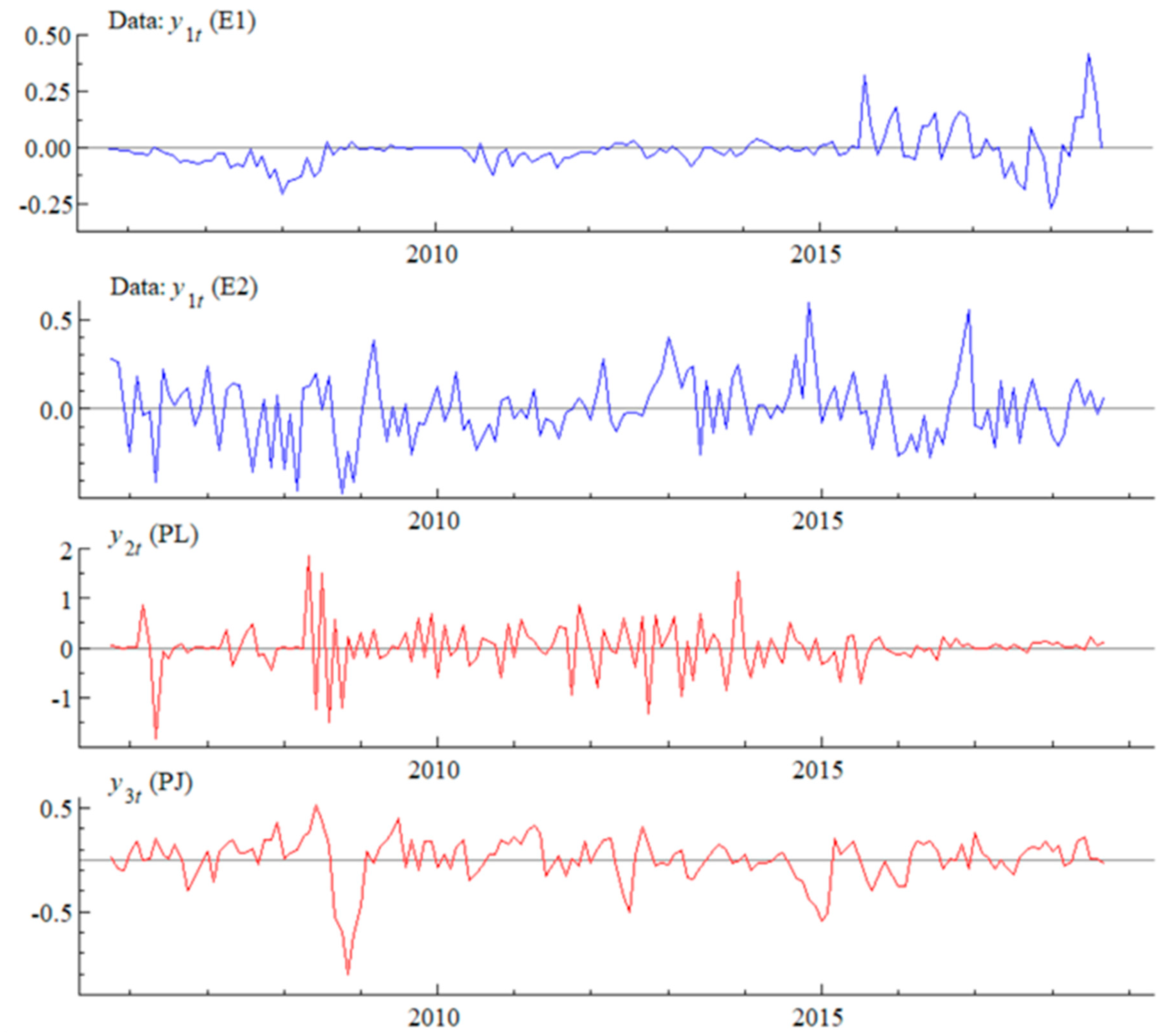
Figure 1 is the plots of the standardized data of our variables calculated from Equation (20). From this figure, we can see that the CNY () is more volatile than the JPY (). It is also discernible from the figure that the China LNG import price () seems to fluctuate along with the Japanese crude oil price ().
4. Results
4.1. Unit Root and Cointegration Tests
Table 2 depicts the results of the unit root tests. The table indicates that all our time series data are non-stationary at their level data but become stationary when first differencing them, suggesting that they are all integrated at order one.
Table 3 and Table 4 show the results of the Johansen test for the CNY and JPY versus the natural gas and crude oil prices. The results of the maximum eigenvalue test suggest that both the CNY and JPY are not cointegrated with the natural gas and crude oil prices based on the 5% significance level. These results point out the validity of using the TVP-VAR model instead of the TVP vector error correction model (VECM).
4.2. MCMC Estimation Results
In the MCMC estimation, we ran 10,000 iterations with a burn-in phase of 1000, and a thinning interval of 10.
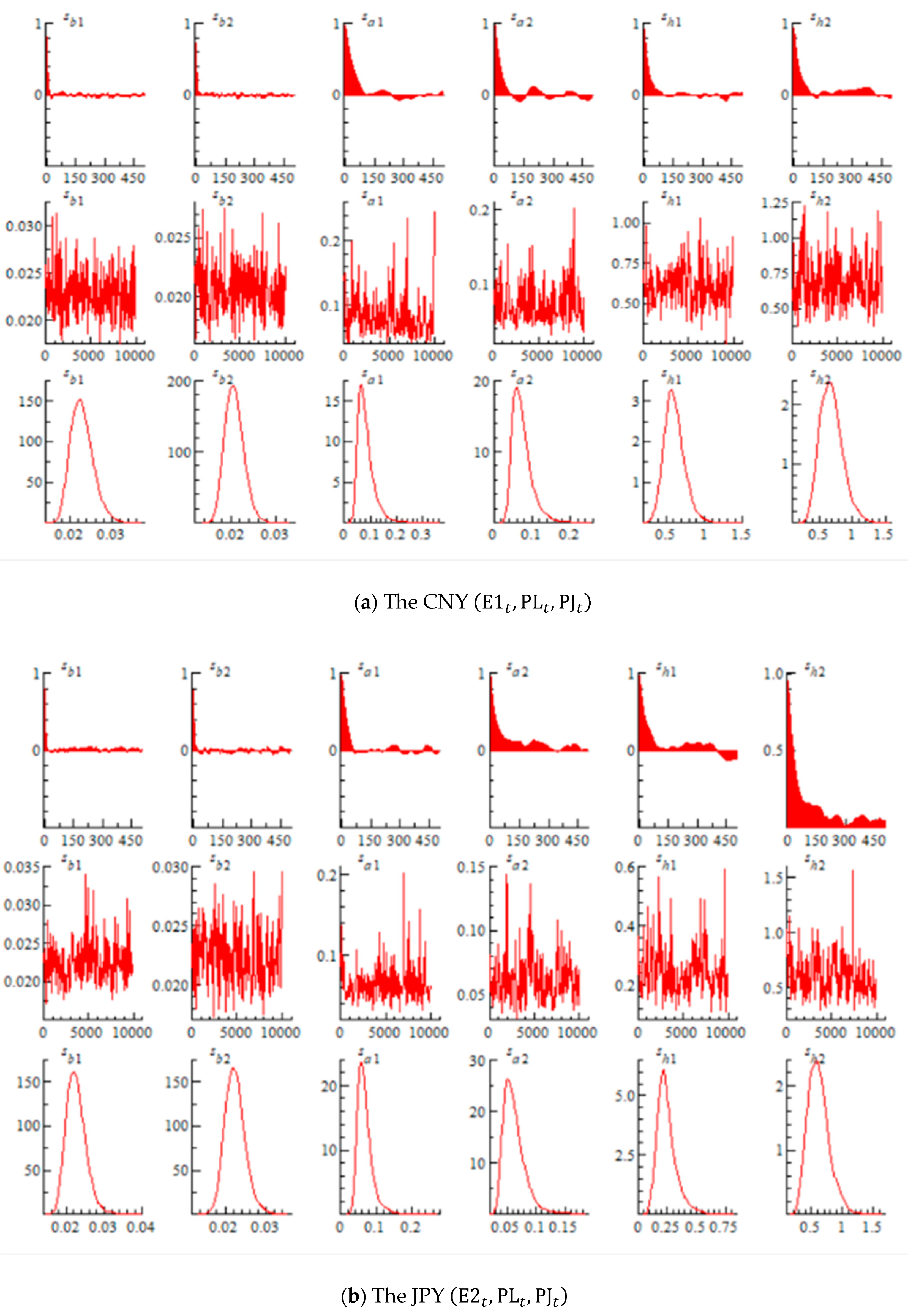
Figure 2 is the sample autocorrelation function (upper), sample path (middle), and posterior probability density function (bottom) of time-varying parameters obtained by the estimation. From the results in Figure 2a,b, both sample paths (middle) converge after 1000 iterations. The sample autocorrelation function shows that both the coefficients (upper) for CNY and JPY were approximately reduced to 0 after 500 iterations. In addition, the results following the normal distribution were obtained for all parameters of the posterior probability density function (bottom).
Table 5 and Table 6 show the posterior mean, standard deviation, 95% confidence interval, Geweke’s convergence decision (CD) statistic (p-value) (Geweke 1991), and the inefficiency factor of the two-sided parameters for the CNY and JPY. Instead of looking directly at the sample path, we used the CD statistics to estimate how many samples were needed to obtain the same variance as the sample mean, which was calculated from the uncorrelated samples. This is called the inefficiency factor. The value of the CD statistics suggests that the model parameters converged to the posterior distribution. As explained before, the CD statistic is the normal distribution statistic of Geweke (1991) for the convergence test and it is known that the Z value of the normal test statistic is 1.6 at the 5% significance level. All the CD test values in Table 5 and Table 6 are above 1.6, indicating that the null hypothesis was not rejected at the 5% significance level. Therefore, the null hypothesis of parameters converging to the posterior distribution was satisfied.
As seen in the tables, the values of the inefficiency factor were all less than 100, which validated the use of the MCMC method (Nakajima and Watanabe 2012). This also confirmed that our posterior distribution sampled 10,000 times from the prior distribution is valid. Based on these results that both of our CNY and JPY samples converge to the posterior distribution, we used the MCMC method for both currencies.
4.3. Results of the Impulse Response Analysis
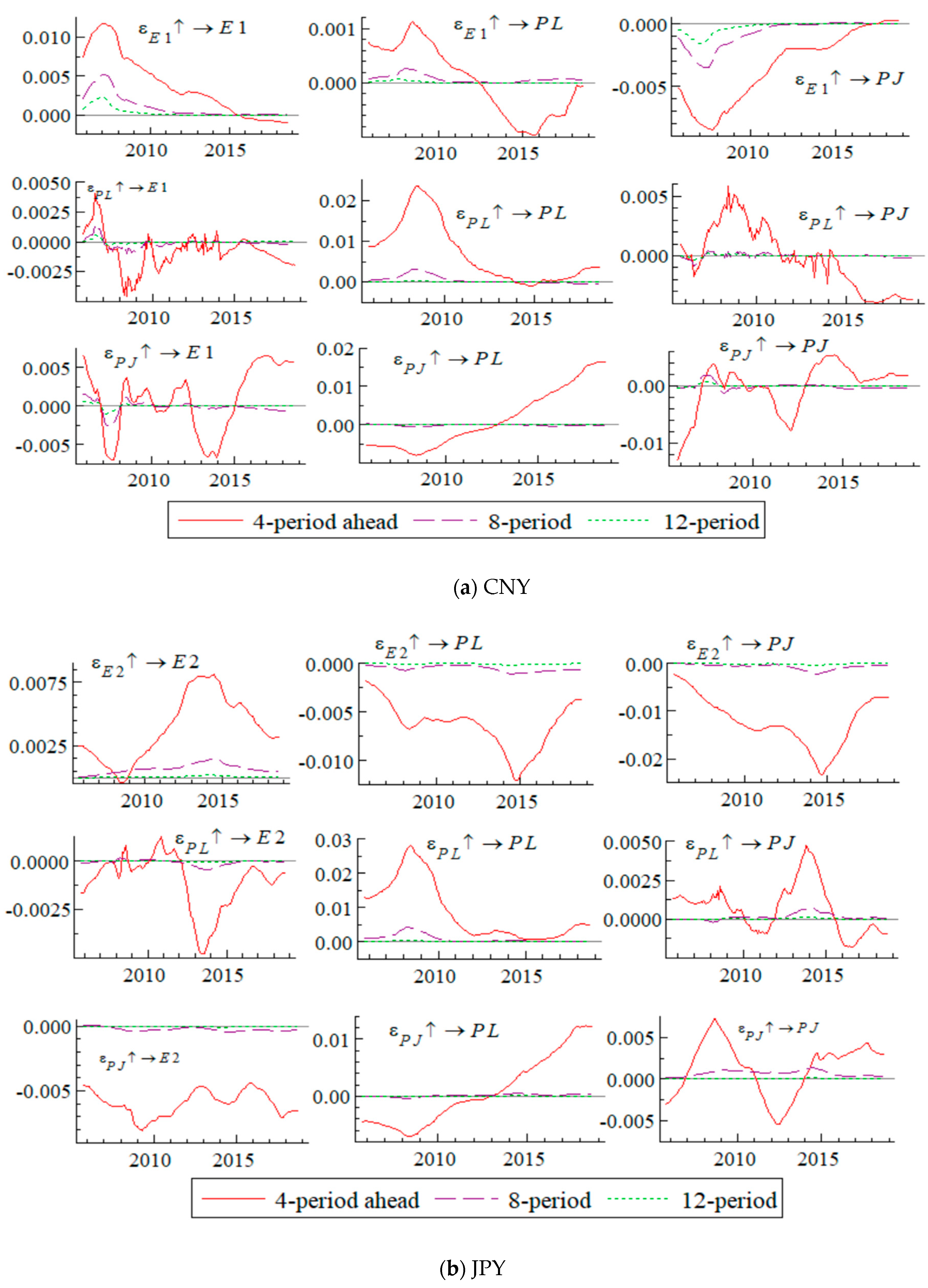
In this section, the impulse response function of the TVP-VAR model is discussed. Since the parameter values of the TVP-VAR model change at each time point, the impulse response function can be drawn in a different diagram at each time period. Figure 3 shows the shock and response of each variable of the time paths from the shock (4th, 8th, and 12th lag periods) at each time period.
According to Figure 3a, the impulse response value of the Chinese LNG import price from the CNY (E1) (4th lag period:) decreased positively from August 2005 to February 2007, but increased in March 2007. As the value of CNY appreciated after the financial crisis, the effects from the CNY on the LNG import price tended to decline from April 2008 to February 2012. However, from March 2012 to September 2018, the value of the Chinese LNG import price from the CNY (4th lag period:) became negative and increased with a negative tendency, and started to decrease toward zero from July 2015. It is discernible from Figure 3a that the CNY negatively affects the JCC crude oil price and the JCC price positively influences the LNG import price, meaning the CNY has negative impacts on the LNG import price.
According to Figure 3b, the impulse response of the Chinese LNG import price against the JPY (E2) for the fourth lag period (4th lag period:) is similar to that of the JCC price against the JPY (E2) (4th lag period:). Both the LNG import price and the JCC crude oil price were negatively correlated with the JPY, suggesting that JPY appreciation may lead to a drop in the Chinese LNG import and JCC crude oil prices. The 4th lag periods for the and between August 2005 to August 2014 have a declining trend, but after September 2014, the impulses from both of the currencies have been increasing toward zero.
Comparing the results of the CNY and JPY in Figure 3, the CNY has a lower impulse response than the JPY on both the LNG import and JCC crude oil prices at the 4th lag period. It is apparent that in both currencies, the impulse response effects at the 4th lag periods are higher than the other lag periods.
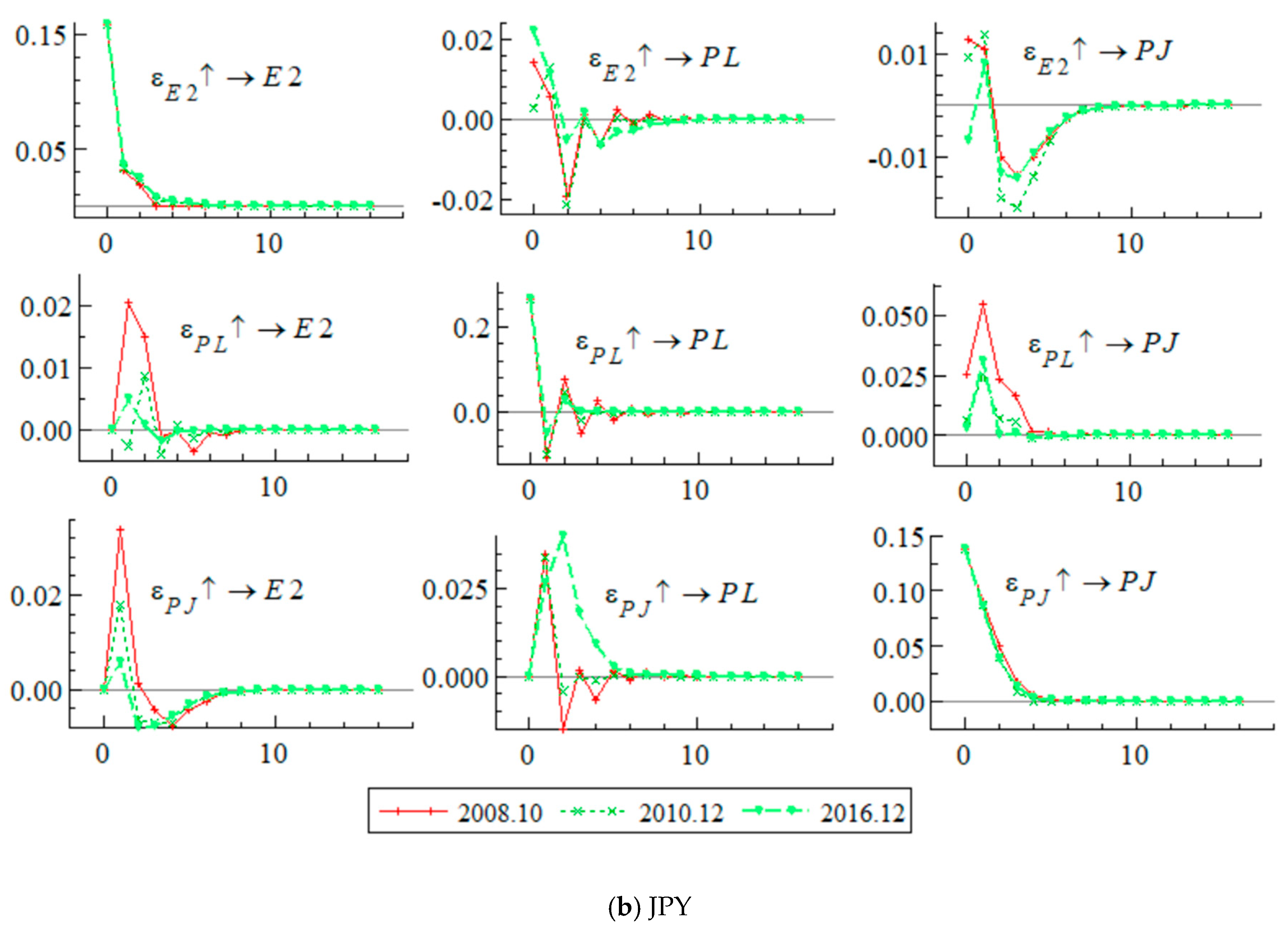
Figure 4 shows the impulse responses of October 2008, December 2010, and December 2016, which are likely to reflect the effects of the CNY monetary reform. According to Figure 4a, the impulse response of the CNY on the Chinese LNG import price () from October 2008 has a higher degree of response than those from December 2010 and December 2016. The reason for this increased impulse from the CNY on the LNG import price might be related to the monetary reform and the shock of the 2008 financial crisis. From Figure 4b, the impulse response of the JPY on the Chinese LNG import price () from 2008 seems lower than those from December 2010 and December 2016. This might be because the JPY had more influence on the LNG import price than the CNY when the 2008 financial crisis occurred. It could be that the JPY was more susceptible to the oil price plummeted after the crisis.
Observing Figure 4 from a comparative viewpoint, the impulse response of JPY to JPY () from October 2008 shows that the impulse stayed relatively stable for December 2010 and December 2016. On the other hand, the impulse response of CNY to CNY () shows that the shock from October 2008 was larger than the shocks from the other two periods. Its lag effect remained up to the 10th examined period. This longer lag effect in the CNY compared to JPY is again likely to be the influence of governmental control regarding the CNY.
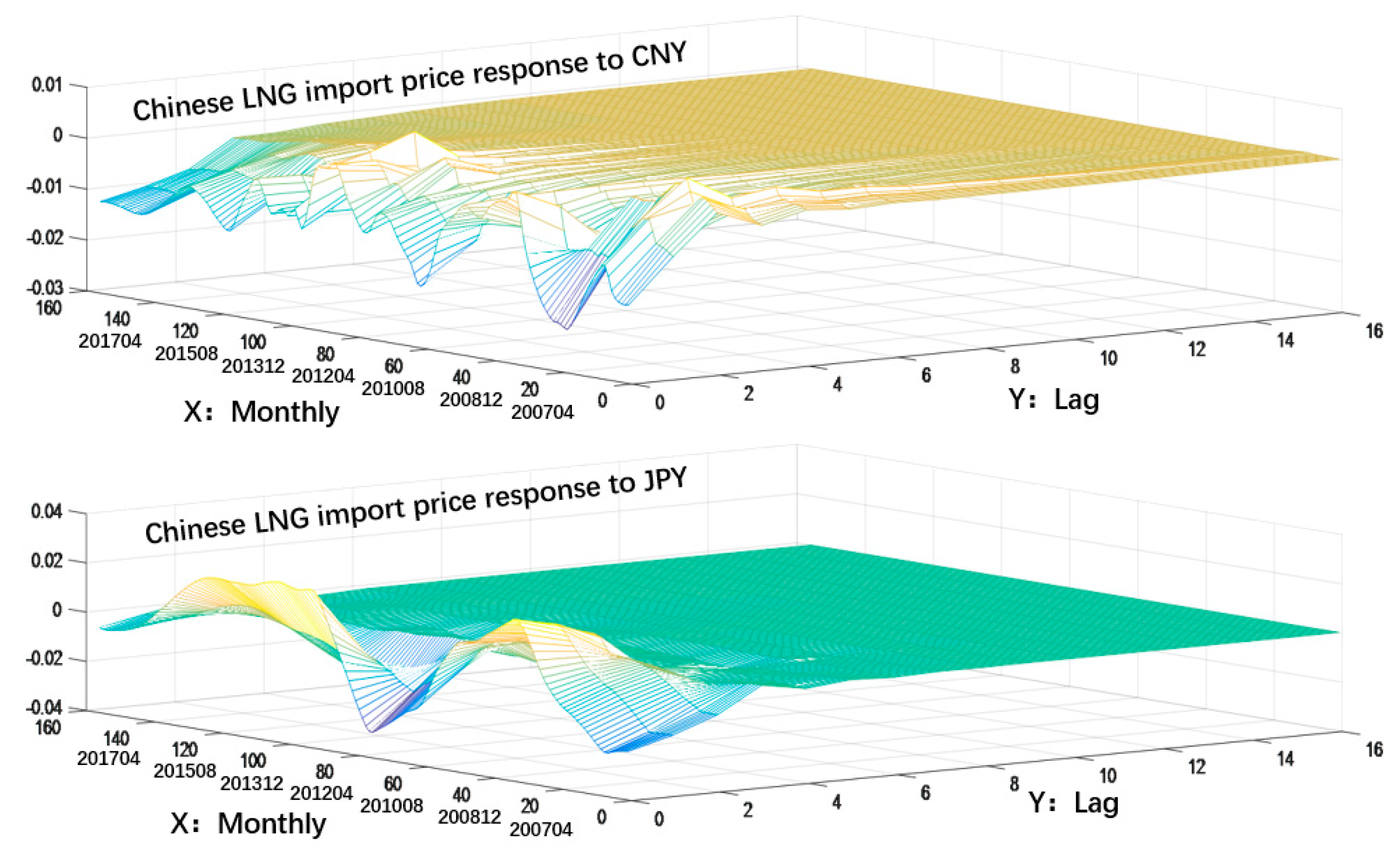
Figure 5 shows the three-dimensional (3D) plot that captures the overall image of the impulse response of the CNY and JPY on the Chinese LNG import price. From the figure, it is observable that the shock from the CNY to the LNG price (upper figure) is stable up until the 6th lag period while the shock from the JPY seems stable only until the 4th lag period. Presumably, the reason for JPY having a shorter time period to absorb the shock is that the JPY is more capable to adjust to the free inflow and outflow of foreign capital while the CNY has been controlled under the regulations imposed by the Chinese government.
4.4. Pass-Through Rate Results
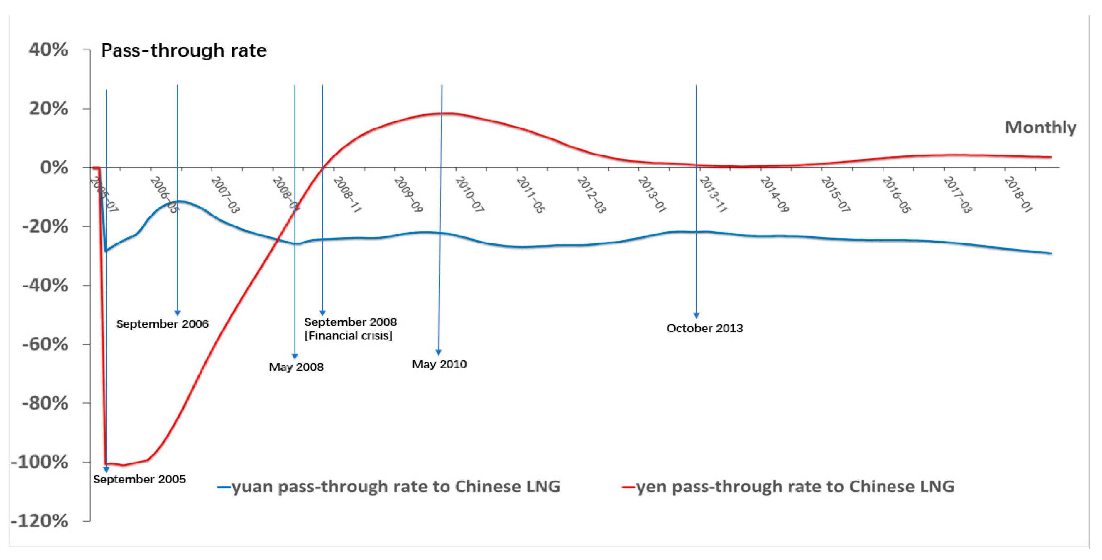
In Figure 6, the pass-through rate was calculated using the cumulative response value of the impulse in the first period from the shock of the CNY and JPY on the Chinese LNG import price.
Let be the pass-through rate of CNY to the Chinese import LNG import price and be the pass-through rate of JPY on the Chinese LNG import price. Then, the figure indicates that from , the pass-through rate of the JPY exceeded −100% in September 2005. On the other hand, the results of the show that the pass-through rate of the CNY in this period was only −25%. The figure illustrates that compared to CNY, the effects of the JPY began to decline after September 2005. decreased to 0% by September 2008, while did not decline by that much and fluctuated at around negative 25% from October 2006 to May 2008.
Then, from September 2008 to May 2010, increased toward a positive direction and reached a maximum of about 20%, while decreased slightly, but then seemed to be stable at around 20%. Besides, decreased to approach 0% from May 2010 to October 2013, while was stable near the 25% level from October 2008 to 2013. However, increased in the negative direction since October 2013, while declined to near zero.
These weakening impacts of JPY on the LNG import price were likely related to the CNY monetary reform. The year 2005 was the year when the Chinese government conducted the monetary reform, so the declining impact of the JPY after 2005 might be indicating that the CNY began to have more influence on the Chinese LNG import market after the monetary reform occurred. It is known that even if the CNY is managed by the government, this reform can be a significant influential factor in import price fluctuations (John et al. 1992). Hence, we conceived that it is reasonable to interpret the fact that the CNY began to play an important role in the Chinse LNG market after 2005 is related to the CNY monetary reform. It is probable that due to the effect of this 2005 CNY reform, the CNY pass-through rate on the LNG import price began to become higher than that of the JPY after 2008 and this higher CNY pass-through rate remained during our investigation period.
5. Discussions
First, the above results of Table 5 and Table 6, and Figure 2 indicate that the parameters of the TVP-VAR model in this study have changed during our test period. This implies that importing companies and suppliers in the international LNG market need to consider the effects of the CNY fluctuations when purchasing LNG. Thus, the study results provide valuable price discovery information for Chinese LNG market stakeholders. Numerous studies indicate that the TVP-VAR model can be applied to analyze macroeconomic data and has its strength in estimating parameters of models that change with time (Primiceri 2005; Nakajima and Watanabe 2012; Shioji and Uchino 2009; Shioji 2010). However, this method has not been applied to understand the relationship between the Chinese LNG import market and the Chinese exchange rate market after monetary reform took place in China. Hence, the current study provides some evidence on how effective the TVP-VAR model can be when analyzing the energy price and currency rate relationship.
Second, Figure 5 revealed that the shock from the CNY to the LNG price (upper figure) was stable up until the 6th lag period, while the shock from the JPY was stable only until the 4th lag period. These results are consistent with the conclusion of Shinkai (2011), Choudhria and Hakura (2015), and Pennings (2017) suggesting that the exchange rate pass-through to import prices is incomplete for a large number of countries. The result of the impulse response analysis indicated that as the volatility of the CNY increased, the exchange rate risk in the LNG trading market gradually transferred from the JPY to the CNY after 2005. The results in Figure 6 also indicate that compared to JPY, the influence of the CNY began to intensify after 2005. These results imply that since the July 2005 currency reform, the impact of the CNY on the LNG import market became stronger. This suggests the importance of considering the effects of monetary reform for understanding the Chinese LNG import and the exchange rate relationship.
6. Conclusions
This paper provided an overview of the empirical methodology of the TVP-VAR model with stochastic volatility, as well as its application to the pass-through rate of the JPY and CNY on the Chinese LNG import price. The empirical application of the TVP regression model revealed the importance of incorporating stochastic volatility into parameter estimation when analyzing the impact of the exchange rate on the LNG import price.
The results of our study indicate that if a new CNY monetary reform takes place in the future, the effects of JPY on the Chinese LNG price will be reduced and those of the CNY on the Chinese LNG price is likely to become stronger. The study suggests the importance of considering the CNY fluctuation range when discovering or forecasting the price of the Chinese LNG import price. These findings imply that the LNG import price will be more stabilized when the CNY is controlled by the Chinese government.
Hence, the study indicates the significance of considering effects of the exchange rate on an energy market when it is likely to be influenced by a monetary reform of the importing country. The study also suggests the importance of applying the TVP-VAR model instead of using the conventional VAR model when the parameters in the VAR model are time-variant.
Finally, our study is limited in a way that it did not consider other factors such as the freight and insurance premiums that could influence the pass-through rate on the LNG import price. Hence, for our future study, we are hoping to investigate the pass-through rate when these factors are considered in the TVP-VAR model
Supplementary Materials
The price data used in this study is available online at https://0-www-mdpi-com.brum.beds.ac.uk/2227-7072/8/4/70/s1, Data S1: data source used in the study.
Author Contributions
Conceptualization, C.T. and K.A.; Data curation, C.T. and K.A.; Formal analysis, C.T.; Investigation, C.T. and K.A.; Methodology, C.T. and K.A.; Software, C.T.; Supervision, K.A.; Writing—original draft, C.T.; Writing—review & editing, K.A. All authors have read and agreed to the published version of the manuscript.
Funding
This research was funded by the 2019-2020 Special Fund from the Research Center for Sustainable Development in East Asia, The Strategic Research Area for Sustainable Development in East Asia, Saitama University, Japan.
Conflicts of Interest
The authors declare no conflict of interest.
References
- British Petroleum (BP). 2014. Statistical Review of World Energy. Available online: http://large.stanford.edu/courses/2014/ph240/milic1/docs/bpreview.pdf (accessed on 7 September 2019).
- British Petroleum (BP). 2015. Statistical Review of World Energy. Available online: http://large.stanford.edu/courses/2015/ph240/zerkalov2/docs/bp2015.pdf (accessed on 5 September 2019).
- British Petroleum (BP). 2019. Statistical Review of World Energy. pp. 20–29. Available online: https://www.bp.com/content/dam/bp/business-sites/en/global/corporate/pdfs/energy-economics/statistical-review/bp-stats-review-2019-full-report.pdf (accessed on 5 December 2019).
- Ceglowski, Janet. 2010. Exchange rate pass-through to bilateral import prices. Journal of International Money and Finance 29: 1637–51. [Google Scholar] [CrossRef]
- Choi, Gobong, and Eunnyeong Heo. 2017. Estimating the price premium of LNG in Korea and Japan: The price formula approach. Energy Policy 109: 676–684. [Google Scholar] [CrossRef]
- Choudhria, Ehsan U., and Dalia S. Hakura. 2015. The exchange rate pass-through to import and export prices: The role of nominal rigidities and monetary choice. Journal of International Money and Finance 51: 1–25. [Google Scholar] [CrossRef] [Green Version]
- Geweke, John. 1991. Evaluating the Accuracy of Sampling-Based Approaches to the Calculation of Posterior Moments. Staff Report 148. Minneapolis: Federal Reserve Bank of Minneapolis. [Google Scholar]
- Hui, Xiao-feng, Yu-hua Wang, and Guang-sen Zhang. 2013. An Empirical Study on the result of the Passthrough of Exchange Rate into Domestic Price Based on VAR Model. Journal of Industrial Engineering/Engineering Management 27: 72–73. (In Chinese). [Google Scholar]
- John, Eatwell, Murray Milgate, and Peter Newman. 1992. The New Palgrave Dictionary of Money and Finance. London: Palgrave Macmillan, vol. 3, pp. 1–61. [Google Scholar]
- Jose, Manuel Campa, and Linda S. Goldberg. 2006. Exchange Rate Pass-Through into Import Prices. Review of Economics and Statistics 87: 1–28. [Google Scholar]
- Kawamoto, Kaoru, and Kenji Tsuzaki. 2007. Market valuation of LNG price formulas. Journal of Japan Society of Energy and Resources 29: 1–7. (In Japanese). [Google Scholar]
- Kosumi, Hideo. 2016. Bayesian Computational Statistics, 4th ed. Tokyo: Asakura Bookstore, pp. 68–100. [Google Scholar]
- Kurtović, Safet, Siljković Boris, Denić Nebojsa, Petković Dalibor, Mladenović Svetlana Sokolov, Igor Mladenovic, and Milovancevic Milos. 2018. Exchange rate pass-through and Southeast European economies. Physica A 503: 400–9. [Google Scholar] [CrossRef]
- Liu, Hai Yue, and Xiao Lan Chen. 2017. The imported price, inflation and exchange rate pass-through in China. Cogent Economics & Finance 5: 1–13. [Google Scholar]
- Marazzi, Mario, Sheets Nathan, Vigfusson Robert, Faust Jon, Gagnon Joseph, Jaime R. Marquez, Martin Rovert, Reeve Trevor, and Rogers John. 2005. Exchange Rate Passthrough to US Import Prices: Some New Evidence. Discussion Paper. Washington, DC: International Finance, vol. 833. [Google Scholar]
- Martono, Jeremia Dwi, and Kentaka Aruga. 2018. Investing the price linkage between Asian LNG spot and East Asian LNG prices and its implications. International Journal of Global Energy Issues 41: 86–97. [Google Scholar] [CrossRef]
- Ministry of Economy. 2015. 2014 Annual Report on Energy (Energy White Paper 2015), Chapter 3, Section 1. Available online: https://www.enecho.meti.go.jp/about/whitepaper/2015html/1-3-1.html (accessed on 8 December 2019).
- Ministry of Economy. 2016. 2015 Annual Report on Energy (Energy White Paper 2016), Chapter 1, Section 3. Available online: https://www.enecho.meti.go.jp/about/whitepaper/2016html/1-1-3.html (accessed on 8 December 2019).
- Nakajima, Jouchi. 2011. Time-Varying Parameter VAR Model with Stochastic Volatility: An Overview of Methodology and Empirical Applications. Institute for Monetary and Economic Studies Bank of Japan E-9: 107–42. [Google Scholar]
- Nakajima, Jouchi, and Toshiaki Watanabe. 2012. Time-Varying Vector Autoregressive Model-Survey and Application to Japanese Macro Data. Kunitachi: Institute of Economic Research, Hitotsubashi University, vol. 62, pp. 193–208. (In Japanese) [Google Scholar]
- National Energy Board (NEB). 2016. The 13th Five-Year Plan for Energy Development. Available online: http://www.nea.gov.cn/2017-01/17/c_135989417.htm (accessed on 15 August 2019). (In Chinese)
- Pennings, Steven. 2017. Pass-through of competitors’ exchange rates to US import and producer prices. Journal of International Economics 105: 41–56. [Google Scholar] [CrossRef]
- Primiceri, Giorgio E. 2005. Time-varying structural vector autoregressions and monetary policy. The Review of Economic Studies 72: 821–52. [Google Scholar] [CrossRef]
- Sasaki, Yuri. 2019. Pass-through effect in which exchange rates are reflected in prices-Is pass-through of Japanese imports declining? Ministry of Finance, Policy Research Institute, Ministry of Finance, Financial Review 136: 118–43. (In Japanese). [Google Scholar]
- Sekine, Toshitaka. 2006. Time-varying Exchange Rate Pass-through: Experiences of Some Industrial Countries. BIS Working Paper. Basel: Bank for International Settlements, vol. 202, pp. 1–34. [Google Scholar]
- Shi, Xunpeng, and Malamakkavu Padinjare Variam Hari. 2016. Gas and LNG trading hubs, hub indexation and destination flexibility in East Asia. Energy Policy 96: 587–96. [Google Scholar] [CrossRef]
- Shinkai, Junichi. 2011. Examination of Pass-through Effect of Exchange Rates in the Pacific Region. Osaka University Economics 61: 37–47. (In Japanese). [Google Scholar]
- Shioji, Etsuro. 2010. Transition of Exchange Rate Pass-Through Rate-Re-Examination with Time-Varying Coefficient VAR. Tokyo: Research Institute of Economy, Trade & Industry, vol. 10, pp. 1–24. (In Japanese) [Google Scholar]
- Shioji, Etsuro, and Taisuke Uchino. 2009. Is the Pass-Through of Exchange Rate and Oil Price Fluctuation Changed? Bank of Japan Working Paper Series; Tokyo: Bank of Japan, vol. 9, p. 1. (In Japanese) [Google Scholar]
- Tong, Xiaoguang, Jiong Zheng, and Bo Fang. 2014. Strategic analysis on establishing a natural gas trading hub in China. Natural Gas Industry B1: 210–20. [Google Scholar] [CrossRef] [Green Version]
- Wind. 2019. Wind Is a Paid Network That Collects Global Economic and Other Data. Available online: https://www.wind.com.cn/en/Default.html (accessed on 5 December 2019).
Figure 1.
The plots of CNY (), JPY ( ), crude oil ( ) and LNG import () prices from August 2005 to September 2018.
Figure 1.
The plots of CNY (), JPY ( ), crude oil ( ) and LNG import () prices from August 2005 to September 2018.

Figure 2.
The sample autocorrelation function (upper), sample path (middle), and posterior probability density function (bottom) of TVP-VAR parameters. , , and are error terms of the original time-varying parameters based on the first sub-samples. , , and are error terms of the original time-varying parameters based on the last sub-samples. The vertical axis of the upper figure is the sample autocorrelation, and the horizontal axis denotes the number of iterations. The vertical axis of the middle figure is the sample path and the horizontal axis is the number of iterations. The vertical axis of the bottom figure is the posterior probability density and the horizontal axis is the deviation from the average.

Figure 3.
Posterior mean of the impulse response functions.

Figure 4.
Posterior mean of impulse response functions.


Figure 5.
3D impulse response functions. This is a 3D diagram created using MATLAB R2016a software. The upper part represents the impulse response function of the Chinese LNG import price for the CNY E1, and the lower part represents the impulse response function of the Chinese LNG import price for the JPY E2. The X-axis (year) represents each time point at the data period, the Y-axis (section) represents the time elapsed from the shock (0–16), and the Z-axis represents the response size (post-shock mean).

Figure 6.
Changes in the pass-through rate for the CNY and JPY .


Table 1.
Sampling steps of the Markov chain Monte Carlo (MCMC) method.
| Steps | Detail of Steps |
|---|---|
| 1 | Set the initial value of . |
| 2 | Sampling from . |
| 3 | Sampling from . |
| 4 | Sampling from . |
| 5 | Sampling from . |
| 6 | Sampling from . |
| 7 | Sampling from . |
| 8 | Back to step 2. |
Table 2.
Unit root tests.
| Variables | Level Data (t-Value) | First Difference Data | ||||
|---|---|---|---|---|---|---|
| ADF | PP | KPSS | ADF | PP | KPSS | |
| E1 | −1.29 | −2.43 | 0.63 | |||
| E2 | −0.16 | −1.34 | 0.18 | |||
| PL | −0.34 | −2.45 | 0.09 | |||
| PJ | −0.46 | −2.19 | 0.07 | |||
* Significant at the 5% significance level.
Table 3.
Results of the Johansen cointegration test for CNY.
| Rank Number | Trace Test Statistic | 0.01 Critical Value | p-Value | Maximum Eigenvalue Test Statistic | 0.01 Critical Value | p-Value |
|---|---|---|---|---|---|---|
| None | 35.46 | 25.86 | ||||
| At most 1 | 19.94 | 18.52 | ||||
| At most 2 | 6.63 | 6.63 |
* Significant at the 5% significance level.
Table 4.
Results of the Johansen cointegration test for JPY.
| Rank Number | Trace Test Statistic | 0.01 Critical Value | p-Value | Maximum Eigenvalue Test Statistic | 0.01 Critical Value | p-Value |
|---|---|---|---|---|---|---|
| None | 35.46 | 12.04 | 25.86 | |||
| At most 1 | 19.94 | 7.29 | 18.52 | |||
| At most 2 | 6.63 | 6.63 |
* Significant at the 5% significance level.
Table 5.
Estimation results of the TVP-VAR model parameters on the CNY.
| Parameter | Average | Standard Deviation | 95%Credit Section | CD | Inefficiency Factor |
|---|---|---|---|---|---|
| 0.023 | 0.003 | [0.018, 0.029] | 9.160 | ||
| 0.021 | 0.002 | [0.017, 0.025] | 6.650 | ||
| 0.082 | 0.032 | [0.043, 0.163] | 70.690 | ||
| 0.074 | 0.026 | [0.040, 0.140] | 51.010 | ||
| 0.610 | 0.132 | [0.385, 0.901] | 41.910 | ||
| 0.686 | 0.168 | [0.397, 1.063] | 56.460 |
* Significant at the 5% significance level. CD is the normal distribution statistic of Geweke’s (1991) convergence test. , , and are error terms of the original time-varying parameters based on the first sub-samples. , , and are error terms of the original time-varying parameters based on the last sub-samples.
Table 6.
Estimation results of the TVP-VAR model parameters on the JPY.
| Parameter | Average | Standard Deviation | 95%Credit Section | CD | Inefficiency Factor |
|---|---|---|---|---|---|
| 0.023 | 0.003 | [0.018, 0.028] | 9.360 | ||
| 0.022 | 0.002 | [0.018, 0.028] | 5.170 | ||
| 0.068 | 0.022 | [0.039, 0.125] | 41.420 | ||
| 0.063 | 0.019 | [0.038, 0.124] | 78.930 | ||
| 0.246 | 0.084 | [0.124, 0.458] | 72.560 | ||
| 0.613 | 0.171 | [0.331, 1.001] | 89.370 |
* Significant at the 5% significance level. CD is the normal distribution statistic of Geweke’s (1991) convergence test. , , and are error terms of the original time-varying parameters based on the first sub-samples. , , and are error terms of the original time-varying parameters based on the last sub-samples.
Publisher’s Note: MDPI stays neutral with regard to jurisdictional claims in published maps and institutional affiliations. |
© 2020 by the authors. Licensee MDPI, Basel, Switzerland. This article is an open access article distributed under the terms and conditions of the Creative Commons Attribution (CC BY) license (http://creativecommons.org/licenses/by/4.0/).
Share and Cite
MDPI and ACS Style
Tang, C.; Aruga, K. A Study on the Pass-Through Rate of the Exchange Rate on the Liquid Natural Gas (LNG) Import Price in China. Int. J. Financial Stud. 2020, 8, 70. https://0-doi-org.brum.beds.ac.uk/10.3390/ijfs8040070
AMA Style
Tang C, Aruga K. A Study on the Pass-Through Rate of the Exchange Rate on the Liquid Natural Gas (LNG) Import Price in China. International Journal of Financial Studies. 2020; 8(4):70. https://0-doi-org.brum.beds.ac.uk/10.3390/ijfs8040070
Chicago/Turabian StyleTang, Chaofeng, and Kentaka Aruga. 2020. "A Study on the Pass-Through Rate of the Exchange Rate on the Liquid Natural Gas (LNG) Import Price in China" International Journal of Financial Studies 8, no. 4: 70. https://0-doi-org.brum.beds.ac.uk/10.3390/ijfs8040070
Note that from the first issue of 2016, this journal uses article numbers instead of page numbers. See further details here.