Analysis of Volatility Volume and Open Interest for Nifty Index Futures Using GARCH Analysis and VAR Model

Abstract

The generalized autoregressive conditional heteroscedastic model (GARCH) is used to estimate volatility for Nifty Index futures on day trades. The purpose is to find out if a contemporaneous or causal relation exists between volatility volume and open interest for Nifty Index futures traded on the National Stock Exchange of India, and the extent and direction of these relationships. A complete absence of bidirectional causality in any particular instance depicts noise trading and empirical analysis according to this study establishes that volume has a stronger impact on volatility compared to open interest. Furthermore, the impulse originating from volatility of volume and open interest is low.

1. Introduction

Futures trading plays an important role in the price discovery process. Volatility in relation to other liquidity variables, such as volume and open interest, is of prime importance to hedgers, arbitrageurs and speculators for developing trading strategies. Volumes traded is a significant parameter as it identifies momentum and confirms a trend. A common observed phenomenon is that if trading volume increases, prices generally move in the same direction. Furthermore, if the Index moves higher in an uptrend, the volume increases as well. Studies suggest that trading volume is positively related to volatility and serves as a proxy for information flow in the market. As new information is received, traders take new positions depending on their judgment of trend and direction. Volatility is an appropriate measure which determines when the market has fully incorporated new information, as it reflects the magnitude of price movements within a stipulated period. Open interest, which represents the number of future contracts outstanding or total number of future contracts that have not been closed out, plays an important role in the prediction of volatility. Bessembinder and Seguin (1993) report an intuitive relation between price volatility and open interest. They study the relations between volume, volatility, and market depth in eight physical and financial futures markets. They suggest that volume shocks have large asymmetric effects on volatility. Furthermore, positive unexpected volume shocks on volatility are larger than the impact of negative shocks, and large open interest lessens volatility. Tseng et al. (2018) state that open interest has significant explanatory power with regard to futures’ realized volatility for CSI 300 Index futures. Ferris et al. (2002) opines that the level of open interest is a good proxy for examining the capital flows into and out of the nearest S&P 500 index futures contract.

As index futures are cash-settled future contracts, they are appropriate for speculation, hedging and arbitrage. However, though previous studies regarding the relationship provides impetus for reasoning and judgement, the relationship between these variables has not reached any consensus and remains intuitive. Girma and Mougoue (2002) opine that factors other than volume affect the persistence of volatility in the futures price they studied, and inefficiency could also be due to the fact that futures traders base their prices on the previous day’s trading volume and open interest as a measure of both market consensus and market depth.

Kumar (2017) is of the view that even though Nifty enjoyed a monopoly, volatility used as a proxy for returns was not resilient due to low trading margins, low availability of credit and a lack of funds available for reinvestment.

High volatility in the underlying index could be attributed to exchange-traded Funds (ETFs), whose demand shock passes on to the underlying index and is a reflection of increased noise trading as suggested by Ben-David et al. (2018). Additionally, cross hedging stock sector risk with Index futures for hedging effectiveness (Hsu and Lee (2018)) has an impact on volatility, and furthermore Chang et al. (2018) document that volatility index (VIX) returns affect ETF returns.

This study focuses on the volatility facet of Nifty Index futures traded on the National Stock Exchange of India (NSE), and analyzes different categories of traders who trade Nifty Index futures.

The first objective is to find a best fit model for the different categories of investors who trade Nifty Index futures so that shocks to the uncertain variance are not firm after considering volume and open interest.

The second objective is to understand the extent to which liquidity factors such as volume and open interest affect volatility.

The third objective is to study whether or not a unidirectional or by directional causality exists between volatility and volume, and between volatility and open interest, and volume and open interest, for the different categories of investors.

The fourth objective is to model unexpected movements in the variables to predict future effects with the help of the impulse response function (IRF).

The literature documents work done with GARCH models on Nifty Index futures. However, this work is unique as we model different trader categories that trade Nifty Index futures. GARCH models are fitted to understand the extent to which previous positive and negative shocks affect the trading dynamics of specific traders by capturing specific details of volatility volume and open interest. Furthermore, the vector autoregressive (VAR) model, the Granger causality effect and Impulse Response Function (IRF) provide additional facets to the core analysis.

Beginning with the introduction, the paper is further organized in the following manner: Section 2 summarizes the literature reviewed; Section 3 provides the data description; Section 4 provides model development and observed findings, and Section 5 concludes.

2. Literature Review

A large proportion of previous studies have documented the relationship between volatility volume and open interesressivet. To a great extent, the literature has documented a positive contemporaneous relation between volatility and volume. Trading volume is affected by returns generated, and is indicative of news percolating in the market. Additionally, volatility is affected by both informed as well as uninformed traders who trade in the market. In accordance to the volatility volume relation documented, evidence is provided by Admati and Pfleiderer (1998), who state that large volumes provide a signal for traders to trade. Hence the effect of price movements depends on volumes traded. Thus, the underlying principle for suggesting this positive relation can be found in the basic supply and demand model, i.e., a change in demand induces a price change.

The causal price relation between volume and volatility is also on account of the mixture of distribution hypothesis (MDH) documented by Clark (1973), Epps and Epps (1976) and Harris (1986). They suggest that the two quantities, volatility (change in stock price) and volume, should be positively correlated because the variance in the price change depending on a single transaction is conditional upon the volume of that transaction. Therefore, the relation between price variability and trading volume is due to the joint dependence of price and volume on the underlying common mixing variable, called the rate of information flow to the market. This implies that price and volume change simultaneously in response to new information.

One line of literature studies the effect on volatility with the introduction of derivative trading. Danthine (1978) suggests that the derivatives market increases the depth of a market and consequently reduces its volatility. In relation to the Indian equity futures markets, T Mallikarjunappa and Afsal (2008) state that the introduction of derivatives does not have any stabilizing (or destabilizing) effect in terms of decreasing (or increasing) volatility. The introduction of derivatives has not brought the desired outcome of a decline in volatility. However, the result of the Chow test for parameter stability clearly indicates structural change in the volatility patterns during the post-futures period. They also opine that a change in the volatility process is not due to the introduction of derivatives, but may be due to many other factors, including better information dissemination and more transparency.

Snehal Bandivadekar and Ghosh (2003) is of a similar view and states that turnover in the derivative market of Bombay Stock Exchange (BSE) constitutes not only a small part of the total derivative segment, but is miniscule as compared to BSE cash turnover. Thus, while BSE Sensex incorporates only the market effects, the reduction in volatility due to the “future’s effect” plays a significant role in the case of S&P CNX Nifty. Manmohan Mall et al. (2011) advocates that volatility in the Indian stock Index futures markets is time-varying with asymmetric effects. Furthermore, bad news on account of the US sub-prime crisis increased volatility substantially.

The sequential arrival information hypothesis proposed by Copeland (1976), and later extended by Jennings et al. (1981), suggests a positive bidirectional causal relationship between the absolute values of price changes and trading volume. As new information that reaches the market is not disseminated to all market participants simultaneously, but to one participant at a time, an initially transitional information equilibrium is established. Only after a sequence of intermediate equilibriums have occurred, is the final information equilibrium established. Therefore, due to the sequence of information flow, lagged absolute returns may have the ability to predict current trading volume, and vice versa. Similarly, the asymmetric information hypothesis has also been suggested by Kyle (1985). Hiemstra and Jones (1994) argued that a sequential information flow results in a lagged trading volume having predictive power for current absolute price changes, and lagged absolute price changes having predictive power for current volume.

De Long et al. (1990) postulate the price–volume relationship in terms of the noise– trader model. Noise traders temporarily miss-price the stock in the short run or base their decisions on past price movements. Hence a positive causal relationship between volume and price changes is consistent with the hypothesis that price changes are caused by the action of noise traders. In the Indian context, Mahajan and Singh (2009) examined the empirical relationship between return, volume and volatility dynamics using daily data from the Indian stock market. They found a positive and a significant positive correlation between volume and return volatility, and evidence of causality flowing from volatility to trading volume. Their study also detected one-way causality from return to volume, which is an indicative of noise trading. In a similar line of study, Deo et al. (2008) found bidirectional causality between returns and volume for Hong Kong, Indonesia, Malaysia and Taiwan stock markets.

As risk is linked to volatility, extensive literature exists which analyzes time series data to analyze the relation between volume volatility and open interest. Susheng and Zhen (2014) used the ARMA-EGARCH model to examine the asymmetric GARCH effect and the impact of volume and open interest on volatility. They found that volume is positively related to volatility and open interest is negatively linked to volatility when lagged volume and lagged open interest is considered.

The most recent literature suggests causality between trading activity and volatility in Nifty Index futures over a multiple time horizon, as studied by Jena et al. (2018).The causality from volatility to open interest signifies the effectiveness of hedging activities. Furthermore, applying the GARCH (1, 1) model, the authors Jena and Dash (2014) confirmed a positive relationship among current open interest and lagged volume inaexgplaining volatility in the Nifty index futures. They opine that short-term future price predictability can lead to effective hedge ratios. Magkonis and Tsouknidis (2017) suggested speculative pressures, as reflected by futures trading volume, and hedging pressures, as reflected by open interest, on account of large and persistent spillovers to the spot and futures volatilities of crude oil and heating oil-gasoline markets, respectively. Floros and Salvador (2016) opined that liquidity variables, namely volume and open interest, account for up to 20% of the variation for some markets, and are important variables causing volatility overall during periods of market stability.

3. Data Description

In this study, we consider two liquidity variables, i.e., trading volume (as a proxy for information arrival) and open interest (to analyze liquidity in the index), and its effect on volatility (the variability of price returns).

Quality data with comprehensive transaction details with respect to volume, volatility and open interest were collected from SEBI on Nifty Index futures. The data span was 1 January 2014 to 31 December 2019, collected from the Securities and Exchange Board of India (SEBI)

We have considered two liquidity variables, volume and open interest, to access the impact on volatility. The majority of future contracts traded in the data are found to be near month contracts, as they are the most liquid. This also shows that the contracts are liquid. The expiration date as specified by NSE is the last Thursday of the month. Furthermore, Nifty, being the benchmark index, has huge volumes traded. Nifty represents 52% of the traded volume of NSE and comprises 63% of the market capitalization of NSE.

To model data for volatility, we assume continuous compounding, and the daily return series are calculated as the first difference in the logarithms of the daily closing prices on Nifty futures index contracts.

Empirical studies have documented three main techniques of assessing volatility, namely, stochastic volatility models, implied volatility using options, or time-series models of returns. In this study we measure volatility (price changes) using a specific class of models based on GARCH specifications (Engle 2001).

To study volume dynamics, a preliminary analysis revealed the demography of the trader, whether domestic or a foreigner, along with the trader category, whether retail or institutional. With this information, the trader category could be split up into six categories, as follows: individuals (Category 1); partnership firms, including Hindu Undivided Families (HUF) (Category 2); public/private companies (Category 3); domestic institutional investors (DII) (Category 4); Non Resident Indians (NRIs), overseas body corporate, foreign direct investments (FDI) (Category 5); foreign institutional investors (FII) (Category 6)

Table 1. Volume traded—index futures.

	Futures	Volume
	Trader Category	All Trades	Percentage
1	Individuals	3,067,836,325	49.583
2	Partnership firms, Hindu Undivided Family, HUF	862,042,950	37.603
3	Public/Private companies	5,049,988,650	18.568
4	Domestic Institutional Investors, DII	82,143,925	4.472
5	NRIs, Overseas Body Corporate, FDI	66,961,850	3.655
6	Foreign Institutional Investors FII	2,671,117,850	0.416
	Full sample	11,800,091,550	23.730

provides details regarding volume traded by the different categories of traders on the NSE (National Stock Exchange of India). We find that individuals constitute the maximum trading volume, and FIIs the least.

Table 2. Descriptive statistics of volatility, open interest and volume in the individual category.

Statistics	Volatility	Volume	Open Interest
Mean	−0.0005	3679578	17340433
Median	−0.0006	3816800	16865106
Maximum	0.0289	8032767	28474865
Minimum	−0.0386	53200	5943600
Standard Deviation	0.0091	2031685	4117847
Skewness	−0.15	−0.28	−0.04
Kurtosis	4.50	2.30	2.71
Jarque-Bera test (p-value)	46.11 (<0.0001) *	15.64 (0.0004) *	1.72 (0.4229) *
ADF (p-value)	−22.74 (<0.0001) *	−1.75 (0.4046) *	−7.01 (0.4046) *
No. of observations	470	470	470

(Figures in parentheses are the p-values).* (The rest of the tables for different categories could be made available on request).

provides descriptive statistics for the volume volatility and the open interest series to get a preliminary understanding of the dynamics between these series.

Each of the six categories of investors is dealt with separately in order to understand the causal relation between the three pairs of variables.

Table 2 represents the summary statistics of the volatility, open interest and volume for individuals. The mean volatility is −0.0005 with a standard deviation of 0.0091. The distribution of volatility is leptokurtic, while volume and open interest show platykurtic distribution. As regards skewness, all series are negatively skewed. The null hypothesis of normal distribution was tested using the Jarque–Bera test, whereby volatility and volume appear statistically significant, indicating non-normal distribution, while open interest accepted the null hypothesis by following normal distribution. ADF statistics of volatility are significant statistically, indicating that volatility is stationary, while volume and open interest series are non-stationary. Index returns are time-varying and highly unrelenting. To verify the stationary state, the Kwiatkowski–Phillips–Schmidt–Shin (KPSS) test was used. The null hypothesis states that data for volatility series are stationary around a mean or linear trend, where mean and variance are constant over time. Analysis revealed that the data were stationary for all categories at level I (0).

4. Model Specification

We fit the best model (symmetric or asymmetric) for different categories of traders. For this purpose, we firstly determine heteroscedasticity and then perform an asymmetric test to determine the best fit GARCH models (Kande Arachchi (2018)).

In order to determine heteroscedasticity, i.e., ARCH effect, we assess the ACF of the squared error term by fitting the ARIMA (1, 1, 2) model. The first lag term of the ACF of the squares of the residual series is significant. Hence heteroscedasticity exists. Additionally, the hypothesis of no ARCH effects up to lag 20 according to the Lagrange multiplier test is rejected. This further confirms the presence of heteroscedasticity.

4.1. GARCH (1, 1) Model:

As heteroscedasticity is confirmed, after a few iterations we find the GARCH (1, 1) model to be the best fit for all categories, except public and private firms.

We fit a GARCH (1, 1) model for all investors. The details of the model specification are depicted in

Table 3. Estimation results of GARCH (1, 1) model for individual investors.

	Parameters	Coefficient	p-Value
Mean Equation	Constant (φ)	0.00069	0.6800
	Volume	0.00000	0.6343
	Open interest	0.00000	0.5156
Variance Equation	constant (ω)	0.00000	0.0319(S)
	ARCH effect (α)	0.09445	0.0013(S)
	GARCH effect (β)	0.86022	<0.0001(S)
	α + β	0.95466
ARCH-LM test for heteroscedasticity
ARCH-LM test statistic (N*R2)	1.5723
p-value	0.2099

S: Significance at 1% level. The empirical results of the GARCH (1, 1) model on volatility in the individual category are accounted for each day. Monthly data were not appropriate for modeling data as the ARCH effect was not present in monthly data as suggested by the heteroscedasticity test with p-value > 0.05 By including both parameters of volume and open interest, the ARCH effect appears in daily data with p-value 0.0001. The sum of the two estimated ARCH and GARCH coefficients (persistence coefficients) in the estimation process is less than one, suggesting that shocks to the conditional variance are not very persistent after taking volume and open interest into account. The ARCH-LM test statistics for all periods did not exhibit an additional ARCH effect (p-value > 0.05). This shows that the variance equations are well specified.

.

Next, we test for asymmetric effects after fitting the symmetric GARCH (1,1) model based on the sign and size bias test (Akpan and Moffat (2017)). The test was run separately for all categories.

The asymmetric effect was found to be significant only for public and private firms.

Table 4. Estimation results of the EGARCH (1, 1) model in public and private firms.

	Parameters	Coefficient	p-Value
Mean Equation	Constant (φ)	−0.00010	0.9516
	Volume	0.00000	0.7949
	Open interest	0.00000	0.6823
Variance Equation	Constant (ω)	−0.51452	0.0178 (S)
	ARCH effect (α)	0.17961	0.0012 (S)
	GARCH effect (β)	−0.07343	0.0333 (S)
	Leverage effect (Υ)	0.96001	<0.0001 (S)
	α + β	0.10618
ARCH-LM test for heteroscedasticity
ARCH-LM test statistic (N*R2)	0.6708
p-value	0.4128

S: Significance at 1% level.

lists the empirical results of the EGARCH (1, 1) model for volatility in public and private firms, as accounted for each day, and monthly data were not appropriate for use modeling data as the ARCH effect was not present in monthly data as suggested by the heteroscedasticity test with p-value > 0.05 by including both parameters volume and open interest. The ARCH effect appears in the daily data with p-value 0.0007. Further, the EGARCH (1, 1) model shows the best fit. The asymmetric (leverage) effect captured by the parameter estimate Υ is positive and statistically significant, suggesting that the positive shocks have a greater impact on volatility than negative shocks after taking both volume and open interest into account. The null hypothesis of no heteroscedasticity in the residuals is accepted, indicating no ARCH effect on residuals (p-value 0.4128).

4.2. VAR Model

In order to understand how volatility responds to volume and open interest, we further analyze our work with a three-variable VAR model of volume, open interest and volatility for individual and all other categories.

As such, we estimate a vector auto regressive model (VAR) model for equations (i) and (ii) when processes are integrated. We test zero-restrictions on a given set of parameters of a VAR specification. First, we check for the order of integration of the time series. Next, we use the Wald test for the unrestricted VAR models, as specified below:

$${\mathsf{\theta }}_{\mathrm{t}}= {\mathsf{\alpha }}_{\mathrm{o}}+{\mathsf{\alpha }}_1{\mathsf{\theta }}_{\mathrm{t}-1}+{\mathsf{\alpha }}_2{\mathsf{\theta }}_{\mathrm{t}-2}+{\mathsf{\alpha }}_3{\mathsf{\theta }}_{\mathrm{t}-\mathrm{p}}+{\mathsf{\beta }}_1{\mathrm{V}}_{\mathrm{t}-1}+{\mathsf{\beta }}_2{\mathrm{V}}_{\mathrm{t}-2}+\cdots +{\mathsf{\beta }}_3{\mathrm{V}}_{\mathrm{t}-\mathrm{p}}+{\mathsf{\epsilon }}_{\mathrm{t}}$$

(1)

$${\mathrm{V}}_{\mathrm{t}}= {\mathsf{\alpha }}_{\mathrm{o}}+{\mathsf{\alpha }}_1{\mathrm{V}}_{\mathrm{t}-1}+{\mathsf{\alpha }}_2{\mathrm{V}}_{\mathrm{t}-2}+{\mathsf{\alpha }}_3{\mathrm{V}}_{\mathrm{t}-\mathrm{p}}+{\mathsf{\beta }}_1{\mathsf{\theta }}_{\mathrm{t}-1}+{\mathsf{\beta }}_2{\mathsf{\theta }}_{\mathrm{t}-2}+\cdots +{\mathsf{\beta }}_3{\mathsf{\theta }}_{\mathrm{t}-\mathrm{p}}+{\mathsf{\epsilon }}_{\mathrm{t}}$$

(2)

where V_t denotes volume, one of the liquidity proxies that is investigated, O_t denotes volatility, p denotes the number of lags and ε_t is an error term. The optimal lag length, p, is determined through an optimization process based on Akaike’s information criterion (AIC).

The null hypothesis of the Granger causality tests is based on non-causality, i.e.,

• “V_t does not Granger-cause θ_t” for the first VAR model and
• “θ_t does not Granger-cause V_t” for the second equation.

This test consists of testing whether all the βi of the model equal 0.

As the Grange causality test is sensitive to lagged differences, we utilize AIC (Akaike information criterion), SC (Schwarz information criterion), HQ (Hannan–Quinn information criterion) statistics to determine the best lagged differences. If the p-value is less than 5% the null hypothesis is rejected.

4.3. Variance Decomposition

We analyze the variance decomposition of the VAR model. A three-variable VAR model of volume, open interest and volatility for the individual group and other categories was built, and the graph of VAR can be provided upon request. An analysis revealed that most variance of volatility (volume or open interest) comes from itself. The impact of volatility on volume is stronger than on open interest, while the impact of open interest on volume is stronger than on volatility.

4.4. Impulse Response

Next, we use the impulse response function to analyze how volatility is affected by volume and open interest for different investors.

The impulse response function (IRF) traces the response of the dependent variable (volatility) in the VAR system to shocks in the error term. Such a shock will change the dependent variable in the current as well as future periods, and also have an impact on the independent variables (volume and open interest). The impacts of the shocks are traced for several periods in the future. The method of decomposition used is the Cholesky decomposition. The impulse response function aids in examining the responsiveness of one standard deviation shock given to the explanatory variable to produce a time path for the dependent variable.

After estimating the VAR, the vector moving average (VMA) is formulated to derive the effects of experimental shocks on the chosen variables over time. The method of decomposition used is the Cholesky decomposition.

Let y_t be a K dimensional vector series given by

$${\mathrm{y}}_{\mathrm{t}}={\mathrm{A}}_1{\mathrm{y}}_{\mathrm{t}-1}+\cdots +{\mathrm{A}}_{\mathrm{p}}{\mathrm{y}}_{\mathrm{t}-\mathrm{p}}+{\mathsf{\mu }}_{\mathrm{t}}=\mathsf{\varphi }\left(\mathrm{B}\right){\mathrm{U}}_{\mathrm{t}}+{\displaystyle \sum }_{\mathrm{t}-1}^{\mathsf{\alpha }}{\mathsf{\varphi }}_{\mathrm{i}}{\mathsf{\mu }}_{\mathrm{t}-1}$$

(3)

$$\mathrm{I}=\left(1-{\mathrm{A}}_1\mathrm{B}-{\mathrm{A}}_2\mathrm{B}\cdots {\mathrm{A}}_{\mathrm{p}}{\mathrm{B}}_{\mathrm{p}}\right)\mathsf{\varphi }\left(\mathrm{B}\right)$$

where the MA coefficient measuring the impulse response is given by covU_t = ∑ ϕ_i.

5. Empirical Findings

The GARCH (1,1) model shows the best model fit. The sum of the two estimated ARCH and GARCH coefficients (persistence coefficients) in the estimation process is less than one (Table 3), suggesting that shocks to the conditional variance are not very persistent after taking volume and open interest into account. The ARCH-LM test statistics for all periods did not exhibit an additional ARCH effect (p-value > 0.05). This shows that the variance equations are well specified.

The Granger causality test explains the relation between volatility volume and open interest for individuals and all categories of traders.

The first column indicates p-values (for causal relations) from volatility to liquidity and vice versa. The second column indicates p-values (for causality) from open interest to volatility and vice versa. The third column indicates the p-value (for causality) from open interest to volume and vice versa for Nifty Index futures.

Table 5. Results of Granger causality test.

	Nifty Index Futures
Causal Relations	Volume—Volatility		Open Interest—Volatility		Open Interest—Volume
Categories	Volume Volatility	Volatility Volume	Open Interest Volatility	Volatility Open Interest	Open Interest Volume	Volume Open Interest
Individuals	0.7532	0.8610	0.9574	0.6424	0.1699	0.4079
Partnership Firms	0.3629	0.2895	0.7016	0.3631	0.2433	0.0411
Public and Private Firms	0.1564	0.0155	0.6522	0.9984	0.2709	0.1002
DII	0.5985	0.7706	0.9692	0.2938	0.4350	0.8465
Overseas Corporate	0.5066	0.6589	0.8557	0.6486	0.6503	0.7458
FIIs	0.2808	0.0801	0.7411	0.0572	0.3886	0.6363

represents the Granger causality test after the VAR model is built between volume, open interest and volatility. Because the Granger causality test is sensitive to lagged differences, we utilize AIC (Akaike information criterion), SC (Schwarz information criterion), and HQ (Hannan–Quinn information criterion) statistics to determine the best lagged differences. The results of Granger causality suggest that, as the p-value is greater than 0.05, we cannot reject any null hypothesis in the above table. Thus, this indicates that for the individual category, volatility cannot be forecasted through volume (and open interest), volume cannot be forecasted through volatility (and open interest), and open interest cannot be forecasted through volatility (and volume)

A unidirectional causality is seen for partnership firms from volume to open interest and for public and private firms from volatility to volume. The Granger causality test reveals the absence of bidirectional causality in any of the above cases. The theoretical explanation for bidirectional causality is that volume, which can be considered as a proxy for information, leads to volatility, i.e., a change in price. Large positive price changes imply higher capital gains, which encourage trade, leading to an increase in volume. However, unidirectional causality implies noise trading.

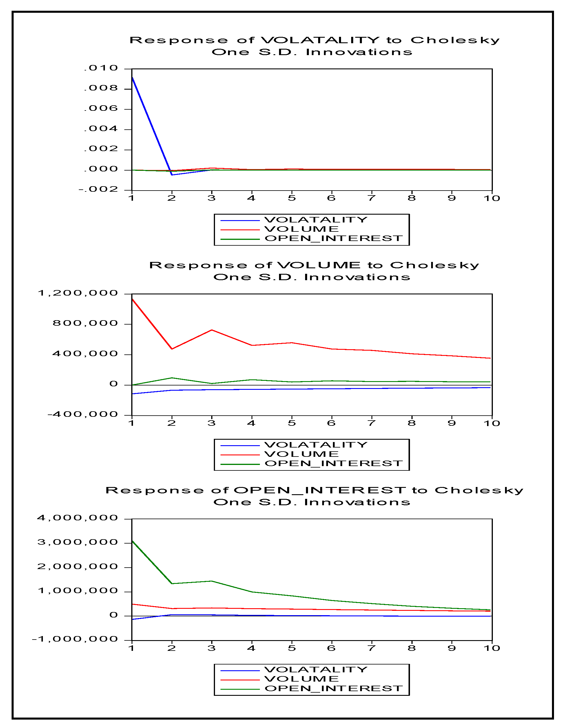
In order to understand the effects on the variables under study of unforeseen conditions, we use the IRF function as depicted in Figure 1.

The time horizon for the impulse response analysis is recorded on the x-axis of each individual graph. The interest of the work is to see the impulse response of a 0.125 unit shock (one standard deviation, SD) innovation to volatility series. The first plot shows the response of volatility to innovation of the volatility series, and the second the response of volume to innovation of the volatility series and the response of open interest to innovation of the volatility series.

When the response of volatility to a one SD innovation is traced (for the individual category), it is found that the volatility series responds negatively to its own innovation. Miniscule negative fluctuations are seen in the second period, and revert to equilibrium by the third period.

In the second graph, volume drops significantly in the second period, then gradually declines and stabilizes by the seventh period.

In the third graph the open interest series is seen declining gradually, and reverts toequilibrium gradually.

The impulse originating from either variable has a tiny effect on the other. Similar to variance decomposition, the impact of the impulse originating from volatility on volume and open interest is low at each period.

6. Conclusions

In this work we have studied the relation between volatility, volume and open interest.

Preliminary investigations revealed that the volatility, volume and open interest data were left skewed. This implies that most futures trades are undertaken for the purpose of hedging. The results show that the GARCH (1,1) model was the best fit for all categories except public and private firms, where an asymmetric EGARCH (1, 1) model is best suited. The sum of the two estimated ARCH and GARCH coefficients (determination coefficients) in the estimation process is less than one, suggesting that shocks to the uncertain variance are not determined after taking volume and open interest into account. As there was no additional arch effect, we state that the model was best fitted to all categories except public and private firms.

To further understand the relationships between volume, open interest and volatility for all investors, we used the VAR model. It was found that most variance of volatility (volume or open interest) comes from itself. Moreover, the impact of volume is stronger than open interest on volatility.

The estimation of Granger causality suggests noise trading, as there is a unidirectional causality only in two cases. A unidirectional causality is seen for partnership firms from volume to open interest, and for public and private firms from volatility to volume. This suggests noise trading.

The absence of bidirectional causality is reported in any particular instance. No bidirectional causal relationships are seen for any of the trader categories between the three pairs of variables.

The impulse response graphs signify that volatility to its own innovation reveals miniscule negative fluctuations. Volume responds more positively compared to open interest to an innovation in the volatility series. For all the categories of traders, volume has a stronger influence on volatility than open interest. The IRF strengthens the direction of the relationships between the three variables, and confirms that volume has a greater influence on volatility than open interest.

These findings from the estimation of the model provide a strong foundation for further non-linear analysis of these relationships. Furthermore, the study reveals that there is market inefficiency in trading Nifty Index futures, and other factors apart from volume traded and open interest should be analyzed in order to understand better the volatility factor.

References

- Admati, Anat R., and Paul Pfleiderer. 1998. A Theory of Intraday Patterns: Volume and Price Variability. The Review of Financial Studies 1: 3–40. [Google Scholar] [CrossRef]
- Akpan, Emmanuel Alphonsus, and Imoh Udo Moffat. 2017. Detection and modeling of asymmetric GARCH effects in a discrete-time series. International Journal of Statistics and Probability 6: 111–19. [Google Scholar] [CrossRef] [Green Version]
- Bandivadekar, S., and S. Ghosh. 2003. Derivatives and volatility on Indian stock markets. Reserve Bank of India Occasional Papers 24: 187–201. [Google Scholar]
- Ben-David, Itzhak, Francesco Franzoni, and Rabih Moussawi. 2018. Do ETFs increase volatility? The Journal of Finance 73: 2471–535. [Google Scholar] [CrossRef] [Green Version]
- Bessembinder, Hendrik, and Paul J. Seguin. 1993. Price volatility, trading volume, and market depth: Evidence from futures markets. Journal of Financial and Quantitative Analysis 28: 21–39. [Google Scholar] [CrossRef]
- Chang, Chia-Lin, Tai-Lin Hsieh, and Michael McAleer. 2018. Connecting VIX and stock index ETF with VAR and diagonal BEKK. Journal of Risk and Financial Management 11: 58. [Google Scholar] [CrossRef] [Green Version]
- Clark, Peter K. 1973. A subordinated stochastic process model with finite variance for speculative prices. Econometrica 41: 135–55. [Google Scholar] [CrossRef]
- Copeland, Thomas E. 1976. A model of asset trading under the assumption of sequential information arrival. Journal of Finance 31: 1149–68. [Google Scholar] [CrossRef]
- Danthine, Jean-Pierre. 1978. Information, futures prices, and stabilizing speculation. Journal of Economic Theory 17: 79–98. [Google Scholar] [CrossRef]
- De Long, J., A. Shleifer, L. Summers, and R. Waldmann. 1990. Positive feedback, investment strategies, and destabilizing rational speculation. Journal of Finance 45: 379–95. [Google Scholar] [CrossRef] [Green Version]
- Deo, Malabika, K. Srinivasan, and K. Devanadhen. 2008. The empirical relationship between stock returns, trading volume, and volatility: Evidence from select Asia–Pacific stock market. European Journal of Economics, Finance and Administrative Sciences 12: 58–68. [Google Scholar]
- Engle, Robert. 2001. GARCH 101: The use of ARCH/GARCH models in applied econometrics. Journal of Economic Perspectives 15: 157–68. [Google Scholar] [CrossRef] [Green Version]
- Epps, Thomas W., and Mary Lee Epps. 1976. The stochastic dependence of security price changes and transaction volumes: Implications for the mixture-of-distributions hypothesis. Econometrica: Journal of the Econometric Society 44: 305–21. [Google Scholar] [CrossRef]
- Ferris, Stephen P., Hun Y. Park, and Kwangwoo Park. 2002. Volatility, open interest, volume, and arbitrage: Evidence from the S&P 500 futures market. Applied Economics Letters 9: 369–72. [Google Scholar]
- Floros, Christos, and Enrique Salvador. 2016. Volatility, trading volume and open interest in futures markets. International Journal of Managerial Finance 12: 629–53. [Google Scholar] [CrossRef]
- Girma, Paul Berhanu, and Mbodja Mougoue. 2002. An empirical examination of the relation between futures spreads volatility, volume, and open interest. Journal of Futures Markets: Futures, Options, and Other Derivative Products 22: 1083–102. [Google Scholar] [CrossRef]
- Harris, Lawrence. 1986. Cross–security tests of the mixture of distributions hypothesis. Journal of Financial and Quantitative Analysis 21: 39–46. [Google Scholar] [CrossRef]
- Hiemstra, Craig, and Jonathan D. Jones. 1994. Testing for Linear and Nonlinear Granger causality in stock price-volume relation. Journal of Finance 49: 1639–64. [Google Scholar] [CrossRef]
- Hsu, Wen-Chung, and Hsiang-Tai Lee. 2018. Cross hedging stock sector risk with index futures by considering the global equity systematic risk. International Journal of Financial Studies 6: 44. [Google Scholar] [CrossRef] [Green Version]
- Jena, Sangram Keshari, and Ashutosh Dash. 2014. Trading activity and Nifty index futures volatility: An empirical analysis. Applied Financial Economics 24: 1167–76. [Google Scholar] [CrossRef]
- Jena, Sangram Keshari, Aviral Kumar Tiwari, David Roubaud, and Muhammad Shahbaz. 2018. Index futures volatility and trading activity: Measuring causality at a multiple horizon. Finance Research Letters 24: 247–55. [Google Scholar] [CrossRef]
- Jennings, Robert H., Laura T. Starks, and John C. Fellingham. 1981. An equilibrium model of asset trading with sequential information arrival. The Journal of Finance 36: 143–61. [Google Scholar] [CrossRef]
- Kande Arachchi, A. K. M. D. P. 2018. Comparison of Symmetric and Asymmetric GARCH Models: Application of Exchange Rate Volatility. American Journal of Mathematics and Statistics 8: 151–59. [Google Scholar]
- Kumar, B. Prasanna. 2017. Derived signals for S & P CNX nifty index futures. Financial Innovation 3: 20. [Google Scholar]
- Kyle, Albert S. 1985. Continuous Auctions and Insider Trading. Econometrica 53: 1315–35. [Google Scholar] [CrossRef] [Green Version]
- Magkonis, Georgios, and Dimitris A. Tsouknidis. 2017. Dynamic spillover effects across petroleum spot and futures volatilities, trading volume and open interest. International Review of Financial Analysis 52: 104–18. [Google Scholar] [CrossRef] [Green Version]
- Mahajan, Sarika, and Balwinder Singh. 2009. The empirical investigation of relationship between return, volume and volatility dynamics in Indian stock market. Eurasian Journal of Business and Economics 2: 113–37. [Google Scholar]
- Mall, Manmohan, B. Pradhan, and P. Mishra. 2011. Volatility of India’s Stock Index Futures Market: An Empiricial Analysis. Researchers World 2: 119. [Google Scholar]
- Mallikarjunappa, T., and E. M. Afsal. 2008. The impact of derivatives on stock market Volatility: A study of the nifty index. Asian Academy of Management Journal of Accounting and Finance 4: 43–65. [Google Scholar]
- Susheng, W. A. N. G., and Y. Zhen. 2014. The dynamic relationship between volatility, volume and open interest in CSI 300 futures market. WSEAS Transactions on Systems 13: 1–11. [Google Scholar]
- Tseng, Tseng-Chan, Hung-Cheng Lai, and Conghua Wen. 2018. The information content of open interest for the realized range-based volatility: Evidence from Chinese futures market. Journal of Economics Finance and Accounting 5: 339–48. [Google Scholar] [CrossRef]
Figure 1.
Impulse response function of volatility, volume and open interest on innovations in the individual category.