Predicting Extreme Daily Regime Shifts in Financial Time Series Exchange/Johannesburg Stock Exchange—All Share Index

Abstract

During the past decades, seasonal autoregressive integrated moving average (SARIMA) had become one of a prevalent linear models in time series and forecasting. Empirical research advocated that forecasting with non-linear models can be an encouraging alternative to traditional linear models. Linear models are often compared to non-linear models with mixed conclusions in terms of superiority in forecasting performance. Therefore, the aim of this study is to build an early warning system (EWS) model for extreme daily losses for financial stock markets. A logistic model tree (LMT) is used in collaboration with a seasonal autoregressive integrated moving average-Markov-Switching exponential generalised autoregressive conditional heteroscedasticity-generalised extreme value distribution (SARIMA-MS-EGARCH-GEVD) estimates. A time series of the study is a five-day financial time series exchange/Johannesburg stock exchange-all share index (FTSE/JSE-ALSI) for the period of 4 January 2010 to 31 July 2020. The study is set into a two-stage framework. Firstly, SARIMA model is fitted to stock returns in order to obtain independently and identically distributed (i.i.d) residuals and fit the MS(k)-EGARCH(p,q)-GEVD to i.i.d residuals; while, in the second stage, we set-up an EWS model. The results of the estimated MS(2)-EGARCH(1,1) -GEVD revealed that the conditional distribution of returns is highly volatile giving the expected duration to approximately 36 months and 4 days in regime one and 58 months and 2 days in regime two. We further found that any degree losses above 25% implies that there will be no further losses. Using the seven statistical loss functions, the estimated $SARIMA(2,1,0)\times {(2,1,0)}_{240}-MS\left(2\right)-EGARCH(1,1)-GEVD$ proved to be the most appropriate model for predicting extreme regimes losses as it was ranked at 71%. Finally, the results of EWS model exhibit reasonably an overall performance of 98%, sensitivity of 79.89% and specificity of 98.40% respectively. The model further indicated a success classification rate of 89% and a prediction rate of 95%. This is a promising technique for EWS. The findings also confirmed 63% and 51% of extreme losses for both training sample and validation sample to be correctly classified. The findings of this study are useful for decision makers and financial sector for future use and planning. Furthermore, a base for future researchers for conducting studies on emerging markets, have been contributed. These results are also important to risk managers and and investors.

1. Introduction

The last decade saw a large number of financial crises in emerging market economies (EMEs) with often devastating economic, social, and political consequences. These financial crises were in many cases not confined to individual economies, but also spread contagiously to other markets. As a result, international financial institutions have developed early warning system (EWS) models, with the aim of identifying economic weaknesses and vulnerabilities among emerging markets and ultimately anticipating such events. As a result, international and private sector institutions have begun to develop EWS models with the aim of anticipating whether and when individual countries may be affected by a financial crisis. The international monetary fund (IMF) has taken a lead in putting significant effort into developing EWS models for EMEs, which has resulted in influential papers by Kaminsky et al. (1998). However, many central banks, such as the United States (US) Federal Reserve and the Bundes bank, academics, and various private sector institutions have also developed models in recent years. Early warning system models can have substantial value to policy-makers by allowing them to detect underlying economic weaknesses and vulnerabilities, and possibly taking pre-emptive steps to reduce the risks of experiencing a crisis. However, the central concern is that these models have been shown to only perform modestly well in predicting crises.

The aim of this paper is to develop a new EWS model for extreme daily losses that significantly improves upon existing models in three ways. First, and most importantly, the paper argues that a key weakness of existing EWS models is that they are subject to what we call a post-crisis bias. This bias implies that these models fail to distinguish between tranquil periods, when the economic fundamentals are largely sound and sustainable, and post-crisis/recovery periods, when economic variables go through an adjustment process before reaching a more sustainable level or growth path. We show that making this distinction using a logistic model tree (LMT) model with two regimes (a pre-crisis regime and post-crisis/recovery regime) constitutes a substantial improvement in the forecasting ability of EWS models.

Second, many financial crises since the 1990’s have been contagious in spreading across the markets. Therefore, another aim of this paper is to apply to EWS models contagion indicators, to measure real contagion channels through trade linkages (direct and indirect) and financial contagion channels via equity market interdependence. We find that, in particular, the financial contagion channel has been an important factor in explaining and anticipating market crises. Third, we uses a data sample of South African stock market with five day frequency, for the period 2010–2020 as the basis for the EWS model estimations. Because the aim of an EWS model is to develop a framework that allows for predicting crises in relatively open economies in the future, it is imperative to use for the in-sample estimation only those crises and country observations that are similar to those that are likely to occur in the future. Therefore, we have started our sample only in 2010, excluding the 1980’s and early 1990’s, during which capital markets were not yet integrated and capital accounts often still closed to foreign investors, also because many countries still experienced hyperinflation in the early 1990’s. Likewise, we have excluded the years immediately following the transition to a free market in Eastern European countries.

To achieve our objective, we propose a hybrid approach to time series forecasting using SARIMA, MS-EGARCH and GEVD. It is often difficult in practice to determine whether a series under study is generated from a linear or non-linear underlying process or whether one particular method is more effective than the other in out-of-sample forecasting. Thus, it is difficult for forecasters to choose the right technique for their unique situations Zhang (2003). Typically, a number of different models are estimated and the one with the most accurate result is selected. However, the final selected model is not necessarily the best for future use due to some potential influencing factors such as sampling variation, model uncertainty, and change in structure. By combining different methods, the problem of model selection can be eased with little extra effort. Second, real-world time series are rarely pure linear or non-linear. They often contain both linear and non-linear patterns. If this is the case, neither SARIMA, MS-EGARCH nor GEVD can be adequate in modelling and forecasting time series since the SARIMA model cannot deal with non-linear relationships while the MS-EGARCH and GEVD alone are not able to handle both linear and non-linear patterns equally well. Hence, by combining SARIMA with MS-EGARCH and GEVD models, will lead us to accurately model complex time series structures. Third, it is almost universally agreed in the forecasting literature that no single method is best in every situation. This is largely due to the fact that a real-world problem is often complex in nature and any single model may not be able to capture different patterns equally well.

lSigauke et al. (2012) used some ARIMA (herein reference autoregressive integrated moving average) model as a benchmark to test the effectiveness of a generalised extreme value distribution with mixed results in order to obtain i.i.d residuals. Many empirical studies including several large-scale competitions suggest that by combining various models, forecasting accuracy can often be improved over individual model without the need to find a ’true’ or ’best’ model Zhang (2003). In addition, the developed hybrid model is more robust with regard to the possible structure change in the data and a basic idea of a hybrid model in forecasting is to use each model’s unique feature to capture various patterns and both theoretical and empirical findings suggest that combining various methods can be an effective and efficient way to improve forecasts.

With the proposed hybrid model, we amalgamate $SARIMA(p,d,q)\times {(P,D,Q)}_S$ to obtain i.i.d residuals while at the same time model seasonally linear structures in a time series. Using the residual of SARIMA, we fit MS-EGARCH-GEVD to model volatility, regime dependence and extreme tail losses. Specifically, we consider a conditional GEVD with a specification that the extreme value sequence comes from an exponential GARCH-type process in the conditional variance structure. The dependence is captured by an appropriate temporal trend in the location and scale parameters of the GEVD. The advantage of a proposed hybrid lies in its ability to capture conditional heteroscedasticity, structural breaks, asymmetric behaviour through an exponential switching GARCH framework, and further models fat-tail and extreme tail behaviour by the use of GEVD. The SARIMA-MS-EGARCH-GEVD modelling approach is believed to perform better in forecasting and it is suited to explain extremes better than the classical MS-EGARCH and SARIMA alone, which cannot capture the tail behaviour adequately with neither normally distributed nor even fatter tailed distributed (e.g., t) innovations as suggested by Calabrese and Giudici (2015). Following Makatjane et al. (2018b), we denote regime classification of SARIMA-MS-EGARCH-GEVD by the following interval [0,1] for low and high regimes in order to develop a dummy variable for the LMT as this model serves as a warning sign model. This study is the first empirical analysis that employs SARIMA, MS-EGARCH in conjunction with the GEVD and LMT models to quantify the likelihood of future extreme daily losses.

Literature Review

The financial chaos that hit developing markets in the latest decades has initiated the need for precise country hazard assessment Fuertes and Kalotychou (2007). In order to explain and predict the crisis of a country, including the currency crises, several models have been developed by a number of studies worldwide. In empirically observing the crisis, it is significant to be indistinct in how a crisis is defined. The models used for determining the early warning signals of extreme daily losses are discussed in this section together with those used for obtaining regime switches of extreme daily losses. Two non-linear models, such as Markov-Switching autoregressive (MS-AR) and Logistic Regression model, have been considered by Cruz and Mapa (2013) with the aim of developing an early warning system model for inflation in the Philippines. The forecasts were combined by the regime switching of inflation and the likelihood of the occurrence of the inflation crisis. However, the results of these authors showed that an outcome of the regime classification appeared to be erratic with regime lasting for a month. By using penalised maximum likelihood methodology, Arias and Erlandsson (2004), in their study of regime switching as an alternative of early warning system of currency crises, found that the method allowed for them to extract smoother transition probabilities than in the standard case, reflecting the need of policy makers to have advance warning in the medium to long term, rather than the short term. See also Abiad (2003).

Two primary issues have been faced by past analysts. Firstly, considerable research has been developed around the significance of precision in deciding the timing and duration of crisis periods. Furthermore, there has been a significant debate by researchers endeavouring to decide the most ideal approach to analyse correlation dynamics before, during, and after these crisis stages Troug and Murray (2020). Scholars, like Forbes and Rigbon (2002), had a problem in accurately determining the crisis. These authors utilised different methods, such as an exogenous and endogenous approach, but all found different results. Moysiadis and Fokianos (2014) noted that a Markov-chain (MC) algorithm has given future states and it is significance while the categorical response variable is lagged. Two reasons arise for the problem caused by a clear categorical time series when it is modelled by Markovian methods. (1) There is a positive non-linear relationship between the order of MC and free parameters, i.e., as the order of the MC accumulates, so does the free parameters. Nonetheless, these free parameters increase exponentially. However, we incorporate the Bayesian approach to restrict these free parameters to increase exponentially, but remain constant over time with non-constant regime switching probabilities (2). The response variable and the covariates that are observed jointly must be a joint flow between them. Of course, this type of determination might be impossible in the stochastic processes of higher time series frequencies. Hence, the proposed Bayesian approach in this study.

Nevertheless, the model that is known as an EWS according to Edison (2002) is engaged for the prediction of crises mainly the financial crises. There are various types of crises, which included the 2008 US financial crises, including currency crises that were studied by Jeanne and Masson (2000), banking crises by Borio and Drehmann (2009), sovereign debt crises and private sector debt crises by Schimmelpfennig et al. (2003), and equity market crises by Bekaert et al. (2014). Therefore, the study extends the current focus of crises to the prediction of extreme daily losses. In developing an EWS for markets crisis, there are three methodologies that are emphasized. These are the bottom-up methodology, the aggregate methodology and the macroeconomic methodology. The odds of extreme market crisis are addressed and the systemic volatility is being activated and signed if the odds become significant. For the second method, the model is applied to data other than individual banking data. On the third method, the focal point is centred in building a relationship between economic variables with the reason that various macroeconomic variables are required to affect the financial system and reflect their own condition.

Davis and Karim (2008) used a multivariate logit model in their comparison study of an early warning system with the aim of relating the likelihood of occurrence or non-occurrence of a crisis to a vector of n explanatory variables. The probability that a dummy variable takes a value of one (crisis occurs) at a point in time was given by the value of a logistic cumulative distribution that was evaluated for the data and parameters at that point in time. Their results showed that the logit model they estimated might be the best model for globally detecting banking crises. Because of small samples and the need to keep the degrees of freedom, Kolari et al. (2002) added to the work of EWS by estimating a stepwise logistic regression in order to identify the subset of covariates that are needed in the model through their power to discriminate. The predefined significance level was set at 10% and the impact of this was that few variables were chosen in the model, hence the need to increase the significance level to 30%, which was used as a threshold to add variables in the model. The main problem that caused the lack of significance of the variables in entering the model is due to the fact that the error term in the regression model followed a cumulative distribution that does not accurately estimate a logit function.

2. Materials and Methods

Let $r_t$ be stock returns at time t, Chinhamu et al. (2015) and Bee (2018) showed that the returns can be modelled by

$$r_t={\mu }_t+{\epsilon }_t,$$

(1)

where ${\mu }_t$ is a time-varying mean and ${\epsilon }_t$ is the error term that can be modelled by

$${\epsilon }_t={\nu }_t{\sigma }_t.$$

(2)

${\sigma }_t$ is the time-varying dynamics, while ${\nu }_t$ is an i.i.d process. The distribution of ${\nu }_t$, specifically its tails, is our focus in this study. We apply block minima (BM) to tails regions of the innovation distribution of Equation (2) and its associated extreme quantiles.

2.1. SARIMA-(p,d,q)(P,D,Q)-MS(K)-EGARCH(p,q)-GEVD

Box et al. (2015) invented two models which are known as SARIMA intervention and SARIMA respectively. Additionally, SARIMA model is proposed in this study to serve as a predecessor that is used to filter a time series in order to obtain i.i.d residuals. According to Makatjane et al. (2018a), a multiplicative SARIMA model denoted by $SARIMA(p,d,q)\times {(P,D,Q)}_S$ follows this mathematical form

$$\Phi \left(\beta \right){\Phi }_S\left({\beta }^S\right){\left(-\beta \right)}^D{r}_t=\Theta \left(\beta \right){\Theta }_S\left({\beta }^S\right){\epsilon }_t$$

(3)

where ${\epsilon }_t\sim i.i.d\left(0,1\right)$ and S is the seasonal length while $\beta$ is the lag operator. Tsay (2014), emphasized that there should be no common factors between the polynomials of seasonal autoregressive (SAR) and seasonal moving average (SMA); if not the order of the model must be in a reduced form. Moreover, SAR polynomials should acquaint with the characteristic equation of SARMA because that is the duty of SAR model Moroke (2014).

Using the residuals of model (3), we fit the MS-EGARCH-GEVD subject to two regimes. The observations fitted on this model comes from the GEVD following an exponential GARCH process that describes a conditional variance of extremes. To account for the leverage effects, we model Equation (2) with respect to a vector ${\theta }_k$ because past negative values have larger stimulus on the conditional volatility than the past positive values of the same magnitude Ardia et al. (2018). Therefore, covariance-stationarity in each regime is accomplished by setting $k>1$ as Ardia et al. (2016) has declared. Hence the MS(k)-EGARCH(p,q)1 is given by

$$ln\left({\sigma }_t^2\right)=\omega +\sum _{i=1}^p\left\{{\alpha }_i\ast \left(\frac{\mid {\epsilon }_{t-i}\mid }{{\sigma }_{t-i}}-\mathbb{E}\left[\frac{\mid {\epsilon }_{t-i}\mid }{{\sigma }_{t-i}}\right]\right)+{\gamma }_i\frac{{\epsilon }_{t-i}}{{\sigma }_{t-i}}\right\}+\sum _j^{q}ln\left({\sigma }_{t-j}^2\right).$$

(4)

Let $S_t$ to be an ergodic homogeneous MC on a finite set, Bauwens et al. (2014) disclosed that $S_t=\left\{1,\dots K\right\}$ and Ardia et al. (2018) defined a transition matrix as $\mathbf{P}\equiv {\left\{p_{ij}\right\}}_{i,j=1}^K$ where $p_{i,j}\equiv P\left[S_t=j\mid S_{t-1}=i\right]$. We initiate the chain at $t=0$ so that ${\left\{S_t\right\}}_{\ge 1}$ is independent from ${\left\{u_t\right\}}_{\ge 1}$. Finally, a time-dependent generalised extreme value distribution is fitted and according to Gagaza et al. (2019) and Coles (2001) this distribution is given by

$$G_{\xi }\left(x\right)=\exp \left\{-{\left[1+\xi \left(\frac{x_i-\mu }{\sigma }\right)\right]}^{-\frac{1}{\xi }}\right\}.$$

(5)

Nonetheless, Equation (5) is valid for $\left\{x:\mu -\frac{\sigma }{\xi }<x<\infty \right\}$, where $\mu$ is the location parameter that ranges from $-\infty <\mu <\infty$ and $\sigma$ is a scale parameter and it must be greater than zero; though $\xi$ is a shape parameter that ranges from $-\infty <\xi <\infty$. When $\xi >0$, a distribution defined in Equation (5) reduces to Fréchet tails, but when $\xi <0$ it corresponds to the Weibull tail type Coles (2001). In order to correct undefined results of distribution (5) when $\xi =0$, we take $\underset{\xi \to \infty }{lim}$ and this results in Gumbel tails.

Once modelling extremes with BM approach, the block size is usually set to one year Nemukula (2018). In this way, the tactic will give only 12 annual maximum or minimum points hereafter, the authors fitted the GEVD to a 30-day (one month) block maxima. But in this study, we use a five-day (five days) blocking to fit the GEVD over a block minima. This is because the stock market data is only observed in a five day period. From each block, the minimas say, $X_i,i=1,\dots ,m$ are selected and this forms a series of m five day minimas to which the GEVD is fitted to. If $X_1,\dots ,X_n$ constitute five day maximum losses that are distributed with the GEVD in model (5), Maposa et al. (2016) showed that in period t, $r_t$ follows $GEVD\left(\mu \left(t\right),\xi ,\sigma \right)$ and Bee (2012) emphasised that $\mu \left(t\right)={\mu }_0+{\mu }_1^t$ for a linear variation in location with an intercept parameter ${\mu }_0$ and a slope parameter ${\mu }_1$, that expresses the rate of change in daily losses. We finally express our proposed hybrid for extreme return losses as $r_t\sim SARIMA\left(p,d,q\right)\times \left(P,D,Q\right)-MS\left(k\right)-EGARCH(p,q)-GEVD\left(xi,{\mu }_t,{\sigma }_t\right)$.

2.2. Logistic Model Tree

The logistic model tree (LMT) is engaged as part of this study to determine an early warning system (EWS) for the extreme daily losses. This method is utilised as a development from the $MS\left(k\right)-EGARCH(p,q)-GEVD$. The regimes are regarded as the binary response variable in an LMT model. The practicality of crises of extreme losses is being assessed through the probabilities that are extracted from the LMT. The logistic model tree is a classification model, which combines decision tree learning methods and logistic regression (LR) Bui et al. (2016). Following Chen et al. (2017), we make use of the LogitBoost algorithm to produce an LR model at every node in the tree, and the tree is pruned using a classification and regression tree (CART) algorithm. The LMT uses cross-validation to find a number of LogitBoost iterations to prevent the over-fitting of training data. The LogitBoost algorithm uses additive least-squares fits of the logistic regression for each $M_i$ class according to Doetsch et al. (2009); it is as follows

$$L_M\left(X\right)=\sum _{i=1}^n{\beta }_i{X}_i+{\beta }_0$$

(6)

where ${\beta }_i$ is the coefficient of the $i^{th}$ component of vector x,whereas n is the number of factors. Furthermore, just as in Chen et al. (2017)’s work, we make use of a linear logistic regression procedure to compute the posterior probabilities of leaf nodes in the LMT model and, according to Agresti (2018) and Stokes et al. (2012), the posteriors are computed by

$$P\left(M\mid X\right)=\frac{\exp \left(L_M\left(X\right)\right)}{{\sum }_{M^{\prime }=1}^D\exp \left(L_{M^{\prime }}\left(X\right)\right)}$$

(7)

where D is the number of classes. For more readings on LogitBoost algorithm, see, for instance, (Pham and Prakash (2019), Pourghasemi et al. (2018), and Kamarudin et al. (2017)), respectively.

2.3. Bayesian Markov-chain-Monte-Carlo Framework

This subsection presents a theoretical overview of the Bayesian Markov-chain-Monte-Carlo (MCMC) on a five day loss frequency modelling. A five day minima $-X_1,\dots ,-X_n$ are i.i.d residuals from the estimated MS (k)-EGARCH (p,q) model for reasonably large n; and, the marginal distribution of each minima is said to be $x_t\sim GEVD\left(xi,{\mu }_t,{\sigma }_t\right)$. For the parametric inference using MCMC, the posterior distribution is computed using the following Bayes’ Theorem 1.

Theorem 1.

$$\pi \left(\theta \mid x\right)=\frac{\pi \left(x\mid \theta \right)\pi \left(\theta \right)}{{\int }_{\Theta }\pi \left(x\mid \theta \right)\pi \left(\theta \right)d\theta }$$

which is usually written as

$$\pi \left(\theta \mid x\right)\propto \pi \left(x\mid \theta \right)\pi \left(\theta \right).$$

Here,xis a vector of observations,$\theta$is a parameter vector, while$\pi \left(\theta \right)$is the prior and$\pi \left(\theta \mid x\right)$is the posterior distribution. Finally,$\pi \left(x\mid \theta \right)$is the likelihood function with the following$\pi \left(x\right)$normalisation constant and$\Theta$is the space parameter.

According to Maposa et al. (2016), a $100\left(1-\alpha \right)\%$ Bayesian credible set C (or, in particular, credible interval) is a subset of the space parameter $\Theta$, such that

$${\int }_C\pi \left(\theta \mid x\right)d\theta =1-\alpha .$$

(8)

If the space parameter $\Theta$ is discrete, the integral in model (8) is replaced by the summation $\left(\sum \right)$. The quantile-based credible interval is such that if ${\theta }_L^{\ast }$ and ${\theta }_U^{\ast }$ are posterior quantiles for $\theta$, where the former is computed by $\frac{\alpha }{2}$ and the latter by $1-\frac{\alpha }{2}$; then, $\left({\theta }_L^{\ast },{\theta }_U^{\ast }\right)$ is a $100\left(1-\alpha \right)\%$ credible interval for $\theta$; hence, the likelihood function for $GEVD\left(xi,{\mu }_t,{\sigma }_t\right)$ is given by

$$\pi \left(x\mid \theta \right)=\prod _{i=1}^k\frac{1}{\sigma }{\left[1+\xi \left(\frac{x_i-\mu }{\sigma }\right)\right]}^{-\frac{1}{\xi }-1}\exp \left\{-{\left[1+\xi \left(\frac{x_i-\mu }{\sigma }\right)\right]}^{-\frac{1}{\xi }}\right\}.$$

(9)

The joint posterior density is

$$\begin{array}{c} \pi \left(\theta \mid x\right)\propto \pi \left(\theta \right)\pi \left(x\mid \theta \right)\\ \pi \left(\theta \mid x\right)\propto \frac{1}{\sigma }\exp \left\{-\frac{1}{2}{\left({\theta }^{\prime }-\vartheta \right)}^T{\sum }^{-1}\left({\theta }^{\prime }-\vartheta \right)\right\}\times {\prod }_{i=1}^K\frac{1}{\sigma }{\left[1+\xi \left(\frac{x_I-\mu }{\sigma }\right)\right]}^{-\frac{1}{\xi }-1}\exp \left\{-{\left[1+\xi \left(\frac{x_i-\mu }{\sigma }\right)\right]}^{-\frac{1}{\xi }}\right\}\\ \pi \left(\theta \mid x\right)\propto \frac{1}{{\sigma }^{k+1}}\exp \left\{-\frac{1}{2}{\left({\theta }^{\prime }-\vartheta \right)}^T{\sum }^{-1}\left({\theta }^{\prime }-\vartheta \right)\right\}\times \exp \left\{{\sum }_{i=1}^k{\left[1+\xi \left(\frac{x_i-\mu }{\sigma }\right)\right]}^{-\frac{1}{\xi }}\right\}\times {\prod }_{i=1}^k\frac{1}{\sigma }{\left[1+\xi \left(\frac{x_i-\mu }{\sigma }\right)\right]}^{-\frac{1}{\xi }-1}\\ \pi \left(\theta \mid x\right)\propto \frac{1}{{\sigma }^{k+1}}\exp \left\{-\frac{1}{2}{\left({\theta }^{\prime }-\vartheta \right)}^T{\sum }^{-1}\left({\theta }^{\prime }-\vartheta \right)-{\sum }_{i=1}^k{\left[1+\xi \left(\frac{x_i-\mu }{\sigma }\right)\right]}^{-\frac{1}{\xi }}\right\}\times {\prod }_{i=1}^k{\left[1+\xi \left(\frac{x_i-\mu }{\sigma }\right)\right]}^{-\frac{1}{\xi }-1}.\end{array}$$

Having the above joint posterior density, a posterior predictive density is used to predict observations of future posterior tail probabilities, $X_0$, as follows

$$Pr\left(X_0>x_0\mid x_1,\dots ,x_n\right)={\int }_{0}Pr\left(X_0>x_0\mid \theta \right)\pi \left(\theta \mid x\right)d\theta .$$

(10)

According to Billio et al. (2018) and Stephenson and Ribatet (2015), Equation (10) becomes

$$Pr\left(X_0>x_0\mid x_1,\dots ,x_n\right)\approx \frac{1}{k-\alpha +1}\sum _{i=1}^{k}Pr\left(X_0>x_0\mid \theta \right),$$

(11)

where $Pr\left(X_0>x_0\mid \theta \right)$ is the GEVD that is evaluated at $t_0$ and $\alpha$ is the burn-in period. Moreover, if $X_N$ is an annual daily maximum losses over some future period of N years, Maposa et al. (2014) showed that a posterior predictive distribution is given by

$$Pr\left(X_0>x_0\mid x_1,\dots ,x_n\right)\approx \frac{1}{k-\alpha +1}\sum _{i=1}^{k}Pr{\left(X_0>x_0\mid {\theta }_i\right)}^N.$$

(12)

2.4. Forecasting Performance and Predictive Accuracy

The forecasting exercise is performed in pseudo-real-time, i.e., the information which is not accessible, is never utilised at the time a forecast is made. For all models, Carriero et al. (2015) utilized the recursive estimation window and assessed their outcomes with root mean squared forecast error (RMSFE). In any case, the present study tails these methods of Carriero et al. (2015) to evaluate the forecasting performance of the proposed models. The root mean square error (RMSE), mean absolute percentage error (MAPE), mean absolute error (MAE), Diebold-Mariano (D-M) and Theil Inequality Coefficient (TIC) are used.

Given the time series ${\mathrm{Y}}_{\mathrm{t}}$ and the estimated ${\widehat{\mathrm{Y}}}_{\mathrm{t}}$, Spyros (1993) defined MAE and MAPE as

$$MAE=\frac{1}{n}\sum _{i=1}^n\left[Y_t-{\widehat{Y}}_t\right]$$

(13)

$$\mathrm{MAPE}=\frac{1}{\mathrm{n}}\sum _{\mathrm{t}=1}^{\mathrm{n}}\left|{\mathrm{Y}}_{\mathrm{t}}-{\widehat{\mathrm{Y}}}_{\mathrm{t}}\right|\ast 100.$$

(14)

Carriero et al. (2015) specified RMSE by

$$RMSE=\sqrt{\frac{1}{n}{\sum }_1^n{\left[Y_t-{\widehat{Y}}_t\right]}^2}$$

(15)

Theil Inequality Coefficient (TIC) has been derived by Theil (1971) as follows

$${\mathrm{U}}_2=\frac{\sqrt{\sum {\left({\mathrm{p}}_{\mathrm{i}}-{\mathrm{A}}_{\mathrm{i}}\right)}^2}}{\sum {\mathrm{A}}_{\mathrm{i}}^2},$$

(16)

where, the P’s and A’s are defined as changes in predictive and actual values, respectively and $0<{\mathrm{U}}_2<1$. By letting ${\mathrm{Y}}_{\left.\mathrm{t}+\mathrm{h}\right|\mathrm{t}}^1$ and ${\mathrm{Y}}_{\left.\mathrm{t}+\mathrm{h}\right|\mathrm{t}}^2$, Diebold (2015) tested the null hypothesis that two or more forecasts have the same accuracy by utilising the following statistic

$$DM=\frac{\overline{d}}{\frac{\sqrt{2\pi {\widehat{f}}_d\left(0\right)}}{T}}$$

(17)

where ${\widehat{f}}_d\left(0\right)$ is a consistent estimate of $f_d\left(0\right)$ which is

$${\widehat{f}}_d\left(0\right)=\frac{1}{2\pi }\sum _{k=-\left(T-1\right)}^{T-1}\Omega \left(\frac{k}{h-1}\right){\widehat{\gamma }}_d\left(k\right).$$

(18)

Note that ${\widehat{\gamma }}_d\left(k\right)=\frac{1}{T}{\sum }_t^T=\left|k\right|+\left(d_t-\overline{d}\right)\left(d_{t-}\left|k\right|-\overline{d}\right)$ and $\Omega \left(\frac{k}{h-1}\right)=\left\{\begin{array}{c}1,for\left|\frac{k}{h-1}\right|\le 1\\ 0,Otherwise\end{array}\right.$. Perceiving that ${\widehat{\gamma }}_d\left(-k\right)=\left(d_t-\overline{d}\right)\left(d_{t-\mid k\mid }-\overline{d}\right)$ and $\Omega \left(\frac{k}{h-1}\right)=0$ for $\mid k\mid >h-1$, Diebold (2015) revealed that

$${\widehat{f}}_d\left(0\right)=\frac{1}{2}\pi \left({\widehat{\gamma }}_d\left(0\right)+2\sum _{k=1}^{h-1}{\widehat{\gamma }}_d\left(k\right)\right).$$

(19)

If $h\ge 1$ then;

$$DM=\frac{\overline{d}}{\frac{\sqrt{{\widehat{\gamma }}_d\left(0\right)}+2{\sum }_{k=1}^{h-1}{\widehat{\gamma }}_d\left(k\right)}{T}}.$$

(20)

Under the null hypothesis, the test statistic DM is asymptotically normally distributed with mean zero and unit variance. The null hypothesis of no difference will be rejected if the computed DM statistic falls outside the range of $-Z_{\alpha }/2$ to $Z_{\alpha }/2$.

3. Results

In this study, we fit $SARIMA(p,d,q)\times {(P,D,Q)}_S-MS\left(K\right)-EGARCH(p,q)-GEVD$ to a five-day FTSE/JSE-ALSI. This is a high frequency time series obtained from the Johannesburg stock exchange for the period of 4 January 2010 to 31 July 2020. This resulted into 2644 observations2. To achieve this task, we use the Bayesian approach to fit a stationary distribution, denoted by $GEVD(\Phi )$. This procedure is executed using various R packages, such as evdbayes of Stephenson and Ribatet (2015), MSGARCH of Ardia et al. (2018), and ismev of Heffernan et al. (2018), among others. As evidenced in

Table 1. Descriptive Statistics for intra-day loses.

	Skewness	Kurtosis	Frosini	Hegazy1	Anderson-Darling
JSE-ALSI	−4.072	5.930	1.357 (0.0002)	0.104 (0.0002)	28.066 (0.0002)

Key: values in () are probability values of Frosini, hegazy1 and Anderson-Darling.

, the distribution of return losses is asymmetric(i.e., negatively skewed); while, on the other hand, kurtosis is above three designating Fat-tailed distribution. A visual inspection of Figure 1 also shows that the largest losses are experienced between the year 2010 and 2018. Nevertheless, Wang et al. (2020) declared that these large losses are caused by a contractionary monetary policy that was implemented by the South African Reserve bank (SARB). In that context, Acharya et al. (2009) also pointed out six events that are linked to these losses. This includes in them and also as commented by the Global Economist

• Repeal of Glass-Steagall act by the Clinton administration. According to Wallison (2011), Glass-Steagall act is one of the biggest post-depression piece of legislations, separating commercial and investment banks. Although this “deregulation” did not repeal the most important section distinguishing the role of commercial and investment banks.
• The surge in a number of sub-prime mortgages as a response to high level of housing speculations and building up of the bubble.
• The creation of new financial instruments which was risky, hard to assess, and shifted the accountability between agents.
• The fall of real interest rate, combined with the Federal Reserves’ expansionary monetary policy.
• Global financial imbalances.

3.1. SARIMA-MS-EGARCH-GEVD Model

To begin our analysis, we first train $SARIMA(p,d,q)\times {(P,D,Q)}_S$ with the ratio of 80% training and 20% validation sets. The aim here is to filter the returns so to obtain i.i.d residuals. Figure 2 shows the plot of residuals demand, the Q-Q plot and their probability density (pd). First and foremost, we applied an augmented Dickey Fuller (ADF) test to a time series with the aim to accommodate the Box-Jenkins methodology. The results of the ADF test provided a sufficient evidence that the FTSE/JSE-ALSI contains unit root with both seasonal and non-seasonal differencing of order one. i.e., $d=1$. The ADF model with intercept plus trend is the one used as its $Pr\left(\tau \right)=0.001$. In this case, a stationary time series is achieved. In model selection, Akaike information criteria (AIC) and Schwartz Bayesian criteria (SBC) congruently advocate that the SARIMA model is of the form $ARIMA(2,1,0)\times {(2,1,0)}_{240}$ which is formulated below as

$$r_t=\left[1-0.498\Phi \ast \ast \ast \left(1\right)(1+0.916\Phi \ast \ast \ast (2\left)\right)(1+0.65\Phi \ast \ast \ast (240\left)\right(1+0.673\Phi \ast \ast \ast \left(241\right)\left)\right)\right]{\epsilon }_t.$$

When diagnosing the estimated SARIMA, all parameter estimates are found significant at 5% level of significance. Additionally, the estimated Q-statistics also gave vast significant evidence that the estimated model is a white noise process with $Pr(Qstatistic=0.1732)$ and ${\epsilon }_t\sim i.i.d(0,0.02978)$. Makatjane et al. (2018a) have suggested that model parameter estimates must be less than one as to deem them to be sufficient and significant.

Using the residuals of the estimated $SARIMA(2,1,0)\times (2,1,0)240$ we fit MS-EGARCH-GEVD subject to two regimes. The results of fitting the MS(2)-EGARCH(1,1) model to the residuals of the SARIMA model using a training data are presented in

Table 2. Naive Bayesian Estimates of MS(2)-EGARCH(1,1).

		Regime 1
Coefficient	Estimate	Std. Error	t-value	p-value
$\widehat{\gamma }$	−0.675	0.003	61.215	0.000
$\widehat{\xi }$	0.039	0.062	91.515	0.000
$\widehat{\alpha }$	−0.148	0.088	147.00	0.000
$\widehat{\beta }$	0.873	0.119	107.29	0.000
$\widehat{\delta }$	1.042	0.198	747.29	0.000
$\widehat{\mu }$	56.10	0.004	37.811	0.000
$\widehat{\nu }$	0.878	0.045	13.025	0.000
		Regime 2
$\widehat{\gamma }$	−0.415	0.004	4.506	0.000
$\widehat{\xi }$	0.132	0.006	6.170	0.000
$\widehat{\alpha }$	−0.165	0.005	30.034	0.000
$\widehat{\beta }$	0.905	0.001	67.067	0.000
$\widehat{\delta }$	6.234	0.002	87.985	0.000
$\widehat{\mu }$	86.24	0.065	60.098	0.000
$\widehat{\nu }$	0.882	0.006	14.056	0.000
$\widehat{\nu }$	0.882	0.006	14.056	0.000
		Transition Probabilities
	Regime 1		Regime 2
	0.9836		0.0164
	0.0306		0.9694

. Setting the number of burns to 10,000 L and the number of MCMC to 510,000 L, we obtained the acceptance rate MCMC sampler of 54.5%. The estimate of a time-invariant mean parameter denoted by $\widehat{\mu }$ is statistically significant. Both the ARCH $\widehat{\alpha }$ and GARCH estimates $\widehat{\beta }$ are significant, indicating the presence of conditional heteroscedasticity effects in each regime. According to Sigauke et al. (2014), this implies that volatility shocks are also persistent. In addition, the estimates of a skewed student-t $\widehat{\delta }$ parameter is positive and statistically significant, signifying non-normal distribution as reported in Table 1; while the estimates of a shape parameter $\widehat{\xi }$ are significant implying dependent volatility in each regime. Finally, the gamma estimate $\widehat{\gamma }$ is statistically significant, meaning that the effect of negative returns’ shocks on the conditional variance is higher returns.

Each of the two regimes identified has a clear economic interpretation. The variance in regime two is higher than that of regime one by 1.42%. This is a clear indication that the conditional distribution is very volatile, and it is subject to regime-shifts with a daily value of 7.36%. Nevertheless, when JSE-ALSI follows the second regime, on daily average, it falls to 9.67%. This means that when the series is in the second regime, its probability to switch to regime one is $P\left(S_t=2\mid S_t=1\right)=0.0164$. 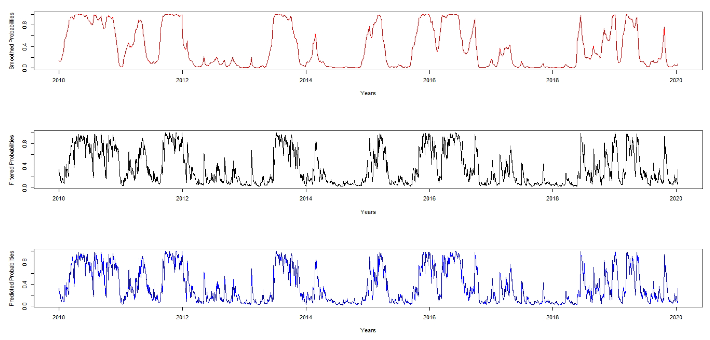The average duration of each regime also supports this behaviour. Based on the expected duration, regime one has approximately 36 months and four days in regime one and 58 months and two days in regime two. Therefore, we conclude that there is a significant regime shifts in JSE-ALI and it can be shown using the filtered and smoothed probabilities in Figure 3.

3.2. Generalised Extreme Value Distribution Framework

Finally, we establish a generalised extreme value distribution. Reported in

Table 3. Naive Bayesian Estimates for Generalised Extreme Value Distribution (GEVD).

	Block	Minima	$\widehat{\mathit{\xi }}$	$\mathit{se}\left(\widehat{\mathit{\xi }}\right)$	$\widehat{\mathit{\sigma }}$	$\mathit{se}\left(\widehat{\mathit{\sigma }}\right)$	${\widehat{\mathit{\mu }}}_0$	$\mathit{se}\left({\widehat{\mathit{\mu }}}_0\right)$	95% CI for $\widehat{\mathit{\xi }}$
JSE-ALSI	2400	482	−0.411	0.024	0.053	0.018	0.071	0.026	( −0.459, −0.363 )

are the MCMC results of the fitted GEVD. As emphasised by Stephenson and Ribatet (2015) and Maposa (2016), näive standard errors are given by dividing the actual standard deviation by the number of iterations. This is due to the fact that Bayesian approach allows for an additional source of variation; probability distributions with hyper parameters and small standard errors. Also, Droumaguet (2012) emphasised that Bayesian methods have densities that solves the problem of confidence interval and allow for model estimation with higher dimensions because some models have complex likelihood function and in practice it becomes difficult to estimate with classical algorithms. Moreover, lSigauke et al. (2012) declared that ambiguity about the parameters is very minimal when using Bayesian approach to model estimation.

The estimate of a shape parameter $\widehat{\xi }$, as shown in Table 3, is negative indicating that FTSE/JSE-ALSI returns conforms to a Weibull class of distribution. The same negative value of the shape parameter is also found in the study of Gagaza et al. (2019) and Sigauke et al. (2014), who found Weibull class in their respective studies. The contrast is in the empirical analysis of Chan (2016) and Coles (2001), where the authors found positive shape parameters in their studies. In-addition, the 95% confidence interval for $\widehat{\xi }$ which is estimated using $\widehat{\xi }\pm z_{\alpha /2}\times \left(standarderror\right)$ has negative interval limits that enclose the estimated shape parameter, hence confirming that the Weibull is an appropriate distribution for FTSE/JSE-ALSI. Gagaza et al. (2019) in their study of modelling non-stationary temperature extremes in KwaZulu-Natal, using the generalised extreme value distribution, found the same negative limits. Furthermore, the right end point is $\mu -\frac{\sigma }{\xi }=1.377113$, which implies that, with any degree losses above 25%, there is unlikely to be any further decrease in JSE-ALSI losses.

3.3. Comparative Analysis

The purpose of this section is to determine the model which best mimics the data and produces fewer forecasts. We therefore, use Akaike information criteria (AIC), Schwartz Bayesian criteria (SBC), mean square error (MSE), mean absolute error (MAE) log-likelihood (LL), mean absolute percentage error (MAPE) and Theil inequality (TIC) which are defined as statistical loss function. The well-known information criterion that are usually used for model selection remain as the criterion used for prediction ability of the estimated models, that is, they are used here to select the model that best predicts the extreme losses. While on the other hand error metrics are used for the forecasting performance. For instance, the log-likelihood selected the best model as SARIMA-MS-EGARCH-GEVD while looking at AIC; the best performing model was also selected as SARIMA-MS-EGARCH-GEVD while MAE and RMSE selected GEVD model as the best model. Therefore, Raihan (2017) in his study, ranked the models according to their statistical loss functions to overcome contradicting results. The author used 10 statistical loss functions. Following this author, we only used seven statistical loss functions and the models were ranked from 1 to 4. On that note, rank 1 denoted the best model while 3 denoted the poorest model.

Table 4. Comparative Analysis.

Test	SARIMA	MS-EGARCH	GEVD	SARIMA-MS-EGARCH-GEVD
LL	708	742	781	622
Rank	2	3	4	1
AIC	−1312	−1455	−1535	−1571
Rank	4	3	2	1
BIC	−1794	−1573	−1653	−1889
Rank	2	4	3	1
MAE	0.9023	0.7988	0.7777	0.7930
Rank	4	3	1	2
MAPE	1.247	1.004	1.002	0.879
Rank	4	3	2	1
RMSE	1.377	1.0016	0.9908	0.9947
Rank	4	3	1	2
TIC	0.6755	0.4155	0.4363	0.4145
Rank	4	2	3	1

gave much evidence that SARIMA model has the poorest performance, as the frequency of rank 4 is higher than the other three models by looking at their statistical loss functions. Nevertheless, the SARIMA-MS-EGARCH-GEVD model outperformed all the models, as the frequency of rank 1 was higher than the other three models as it recorded 5 out of 7 statistical loss functions.

3.4. Evaluation of the Performance of the Logit-Based EWS Model

Several measures are used to evaluate the outcomes of classification algorithms relying on the classified instances Ghatasheh (2014). After processing the input instances, each one is classified into one of four the possibilities that are visually presented in a matrix, by confronting the actual and predicted instances.

Table 5. Probabilities of correct and incorrect predicted Extreme daily.

	High Extreme Losses	Low Extreme Losses
Signal Issued	$P\left(1,1\right)$ Correct call of Losses [A]	$P\left(1,2\right)$ Type II Error or Wrong Signal [B]
No Signal Issued	$P\left(2,1\right)$ Type I error or Missing Signal [C]	$P\left(2,2\right)$ Correct call for non-event [D]

represents the matrix that is called the “Confusion or Contingency Matrix” to perform this task.

In Table 5, event A epitomizes the occasion when the model indicates a crisis when a high inflation event indeed occurs. Event B refers to an event when a signal that is issued by the model is not followed by the occurrence of high inflation, i.e., wrong signal. It is also possible that the model does not signal a crisis (low estimated probability), but a crisis, in fact, occurs, i.e., missing signal, event C. Finally, Event D indicates a situation in which the model does not predict a crisis and no crisis occurs. In this paper, a threshold value of 0.5 is used to indicate whether the probabilities can already be interpreted as crisis signals. To evaluate the EWS model performance, we make use of the following performance criteria that were recommended by Kaminsky et al. (1998).

• Probability of extremes correctly called (PECC):$\frac{A}{B+C}$
• Probability of non-extremes correctly called (PNECC):$\frac{D}{B+D}$
• Probability of observations correctly called (POCC): $\frac{A+D}{A+B+C+D}$
• Adjusted noise-to-signal ratio (ANSR): $\frac{B}{B+D}/\frac{A}{A+C}$
• Probability of an event of high extremes given a signal (PRGS): $\frac{A}{A+B}$
• Probability of an event of high extremes given no signal (PRGNS): $\frac{C}{C+D}$
• Probability of false extremes to total extremes (PFE): $\frac{B}{A+B}$

The performance assessment results of the Logit based EWS model are given as a summary in

Table 6. Probabilities of correct and incorrect predicted Extreme daily.

Training Data	High Extreme Losses			Low Extreme Losses		Total
Predicted	High Extremes	1200	(63% )	398		1598
	Low Extremes	703		106	(21%)	809
Total		1903		504		2407
Validation data	High Extreme Losses			Low Extreme Losses		Total
Predicted	High Extreme Losses	210	(51%)	99		309
	Low extreme Losses	204		16	(14%)	220
Total		414		115		529

The first set of numbers represents counts while figures in parentheses represent percentages of correctly predicted extreme losses.

and

Table 7. Performance of the EWS.

	Training Data	Validation Data
PECC	63%	51%
PNECC	85%	98%
POCC	67%	86%
ANSR	78%	99%
PRGS	43 %	57%
PRGNS	29%	48%
PFE	21%	14%

. We further adopt the following scenarios, as presented by Kaminsky et al. (1998).

The results in Table 6 infer that the model has some EWS potential. In view of the training set estimates, the model has a capacity to accurately predict 63% of high extreme losses and 21% of low extreme losses. As it is, the proportion of high extreme losses, given a signal, is relatively high at 43% in the training sample while the validation sample is at 57%. The proportion of false extremes to total extremes shown in Table 7 is relatively low, at 21% for the training data and 14% for validation data.

The results in Table 7 indicate that there is 51% chance of high extreme losses in the next five years and this probability is about 12% lower than the current situation. The implication here is that the countries’ financial markets could expect investment losses in the future. This inference is made based on the presented validation data estimates. In addition, the proportion of expected false alarm (PFE) to the total alarm is premeditated as 21% which is higher than that of the validation data by 7%. The validation data percent of the non-extremes correctly called is 98%, which 13% higher than that of the training sample. One could conclude that, after all, extreme losses could be low in future.

3.5. Model Performance Evaluation

Ideally, the model-calculated-probability-scores of all actual positives (also known as Ones) should be greater than the model-calculated-probability-scores of all the negatives (also known as Zeroes). Such a model is said to be perfectly concordant and a highly reliable one. This phenomenon can be measured by concordance and discordance. In simpler terms, of all combinations of 1–0 pairs (actuals), concordance is the percentage of pairs, whose scores of actual positives are greater than the scores of actual negatives. For a perfect model, this will be 100%. Accordingly, the higher the concordance, the better the quality of model. In this case, our EWS model is found to be a good model for predicting extreme losses in FTSE/JSE-ALSI with a concordance of 89.15% and the area under curve (AUC) being 88.78%. All of the numbers in

Table 8. Sensitivity Performance of EWS.

	Validation Data
Concordance	89.15%
AUC	88.78%
Sensitivity	79.89%
Specificity	98.40%

are computed using validation data that were not used in the training model Hence, a truth detection rate of 79% on validation data is good, hence our model is a good EWS model for extreme losses.

4. Conclusions and Recommendations

This paper makes use of a stochastic econometric model and extreme value theory (EVT) procedures to establish an early warning system for extreme daily losses stock markets. The statistical input of this work lies in establishing a hybrid model MS(2)-EGARCH(1,1)-GEVD for predicting the extreme losses and to implement the estimated regimes in LMT. To achieve our objective, we set-up a two stage procedure. In the first stage, we train the MS(k)-EGARCH(p,q)-GEVD with 80% training set and 20% validation set. Therefore, we finally use the regime switching of this model to establish the logistic model tree in order to set-up an early warning system. Robust parameter estimates were achieved by using Bayesian MCMC procedure and setting number of burns (nburn) and number of MCMC replicate to $nburn$ = 100,000 L and $nmcmc$ = 510,000 L, respectively. This gave us an overall acceptance rate sampler of 55%; an acceptance rate for the location parameter to be 46.3% and, for the shape parameter, we had a 51.61% acceptance rate.

This study is innovative in a sense that no similar study has used the $SARIMA(p,d,q)\times (P,D,Q)MS\left(k\right)-EGARCH(p,q)-GEVD$ together with the LMT in predicting the possibility of extreme daily losses; and to our knowledge thus far, this study is the first to use the proposed models. Estimation of these models has delivered enhanced understanding of prediction and classification of extreme daily losses. In particular, the study is unique in terms of uniting univariate methods in predicting periods of high and low extreme daily losses. Jointly, the results can be useful in guiding policy-makers in identifying episodes of high extreme losses and safeguard the extreme crisis well ahead of time. In order to optimally classify extreme crises, the LMT is estimated. The two regime probabilities from the $SARIMA(p,d,q)\times (P,D,Q)MS\left(k\right)-EGARCH(p,q)-GEVD$ model are incorporated in the logistic model tree as the binary dependent variable. The low extreme regime was denoted as zero and high extreme regime denoted as one. The study here addresses the events of high and low extreme losses accordingly and found that for the training set, the model has indicated that probability of high extreme losses is 63% while using a validation set was found to be 51% for the next five years.

Stock market participants can use these results to quantify daily operational losses and further predict the probability of default in stock markets. It would be interesting to see what sort of results we get if more sophisticated machine learning methods are used to filter the series and quantify the possibility extreme losses and undertake a comparative analysis with the hybrid MS(k)-EGARCH(p,q)-GPD through the use of MCMC and bootstrapping of the credible confidence interval for returns losses. A probabilistic description and modelling of extreme peak loads using Poison point process is another area that requires future research. This approach helps in estimating the frequency of occurrence of peak losses. A sensitivity analysis with respect to daily losses performed and the development of a two-stage stochastic integer recourse models with the objective of optimising returns’ distribution is an interesting future research direction with stock market data. This will be studied elsewhere.