Assessing Market Risk in BRICS and Oil Markets: An Application of Markov Switching and Vine Copula

Abstract

This paper investigates the dynamic tail dependence risk between BRICS economies and the world energy market, in the context of the COVID-19 financial crisis of 2020, in order to determine optimal investment decisions based on risk metrics. For this purpose, we employ a combination of novel statistical techniques, including Vector Autoregressive (VAR), Markov-switching GJR-GARCH, and vine copula methods. Using a data set consisting of daily stock and world crude oil prices, we find evidence of a structure break in the volatility process, consisting of high and low persistence volatility processes, with a high persistence in the probabilities of transition between lower and higher volatility regimes, as well as the presence of leverage effects. Furthermore, our results based on the C-vine copula confirm the existence of two types of tail dependence: symmetric tail dependence between South Africa and China, South Africa and Russia, and South Africa and India, and asymmetric lower tail dependence between South Africa and Brazil, and South Africa and crude oil. For the purpose of diversification in these markets, we formulate an asset allocation problem using raw returns, MS GARCH returns, and C-vine and R-vine copula-based returns, and optimize it using a Particle Swarm optimization algorithm with a rebalancing strategy. The results demonstrate an inverse relationship between the risk contribution and asset allocation of South Africa and the crude oil market, supporting the existence of a lower tail dependence between them. This suggests that, when South African stocks are in distress, investors tend to shift their holdings in the oil market. Similar results are found between Russia and crude oil, as well as Brazil and crude oil. In the symmetric tail, South African asset allocation is found to have a well-diversified relationship with that of China, Russia, and India, suggesting that these three markets might be good investment destinations when things are not good in South Africa, and vice versa.

1. Introduction

Understanding the complex dependence structure and marginal risk characteristics between BRICS stock indices (Brazil, Russia, India, China and South Africa) and the crude oil/energy market (e.g.,West Texas Intermediate (WTI) crude oil) is central in empirical finance primarily for risk management. For international investors, researchers and policymakers, this could provide crucial information to construct and allocate wealth to well-diversified asset portfolios. While a number of studies have analyzed this relationship and the impact of oil price changes on equity markets (see, for example, Lin et al. (2021); Umar (2017); Apergis and Miller (2009)), the literature on investigating the combined impact of regime-switching volatility and multivariate copula dependence relationship remains sparse.

By the same token, government regulatory institutions and policymakers have the responsibility of ensuring the financial sustainability of the economy, where crude oil is one of the most essential global traded commodities driving economic growth. Crude oil functions as the underlying asset class in the pricing of other financial assets. For instance, the current global food supply chain is highly dependent on fuel and the logistics transport systems. Hence, from an economic standpoint, volatility in crude oil prices can have a major impact on the global economy, with the potential to drive food prices higher, thereby inducing inflation and increased volatility in financial markets (see, for example, Nguyen and Bhatti (2012)).

In wealth allocation and risk diversification strategies, investors are more sensitive to portfolio downside risk than the upside risk. Hence, they are more risk-averse to extreme negative returns and negative market sentiments, which induces herd behavior in stock markets, consequently driving market volatility. The current global pandemic caused by the coronavirus (aka COVID-19), coupled with oil price wars, has increased market volatility, impacting portfolio performance and balance sheets gearing (leverage) ratios. Furthermore, this has led to increased uncertainty about the dependence structure between the recent oil price shocks and their impact on stock market performance in developing economies, primarily due to their heavy reliance on oil as a commodity.

It has been well-documented that portfolio embedded risk measures are directly associated with the dependence structure of portfolio risk factors (see, Brechmann and Czado (2013); Kole et al. (2007)). For example, Junker and May (2005) alluded to the fact that, when aggregating financial risk on a portfolio, it is important to understand the dependence structure among risk factors. Since the establishment of BRICS group economies in 2009, several empirical studies have been conducted using novel methodological approaches, to understand the contagion and spillover effects in BRICS economies with other financial markets and, in particular, other alternative asset classes such as precious metals and cryptocurrencies (see, Jiang et al. (2019); Peng (2020); Thampanya et al. (2020)).

At the center of these lie the multivariate generalizations of GARCH models, first introduced by Bollerslev (1990) and Engle (2002), along with a number of other researchers in the field, who have attempted to address the existence and persistence of the conditional volatility problem in financial assets and how it helps in portfolio diversification and asset allocation. These models have undoubtedly emerged as the most popular tools that offer flexibility for capturing the dynamics of conditional variance and covariance between markets and, in turn aid with the interpretation of the multifaceted dependence structure.

For instance, a study by Morema and Bonga-Bonga (2020) used a vector autoregression asymmetric and dynamic conditional correlation generalised autoregressive conditional heteroskedasticity (VAR-ADCC- GARCH) method to assess volatility spillovers and hedge effectiveness between gold, oil, and stock markets. They find significant volatility spillover between the gold and stock markets, oil and stock markets. Salisu and Gupta (2020) employed the GARCH–MIDAS (Generalized Autoregressive Conditional Heteroskedasticity variant of Mixed Data Sampling) model to investigate volatility transmission from BRICS to oil shocks, and found mixed responses of stock volatility to oil shocks. Meanwhile, Bonga-Bonga (2018) assessed the extent of financial contagion between South Africa and other BRICS countries with VAR-DCC-GARCH, and found evidence of cross-transmission and dependence between South Africa and Brazil. Hassan et al. (2020) estimated volatility spillover in Islamic and conventional stock indices and crude oil in BRICS, using Threshold GARCH (TGARCH) and generalized forecast error variance decomposition. They found that significant volatility spillover exists among crude oil, conventional, and Islamic stock, and suggested that investors rebalance portfolios regularly.

Contrary to what others have done, our study contributes to the existing literature on BRICS and oil markets by using novel approaches, in order to overcome some of the weaknesses of traditional methods. These include methods, such as the multivariate-GARCH models which postulate that assets returns follow a multivariate Gaussian distribution or multivariate-Student t distribution (see, for example, Weiß (2013); Aas and Berg (2009)). Multivariate data sets typically presents complex dependence structure, mostly in the lower and upper tails combined with possible structural breaks which cannot simply be accounted for by the traditional multivariate Student t and Gaussian distributions. Furthermore, our approach models portfolio risk by incorporating asset dependence structure under specific market conditions.

Hence, in this study, we employ a Vector Auto Regressive (VAR) model to account for the joint dependence in the mean returns followed by a Markov switching GJR-GARCH to account for regime changing parameters in the volatility dynamics. In addition, we use multivariate vine copula models to account for various dependence patterns in the tail distributions that exist between BRICS economies and the world energy market. The results are then applied to a portfolio optimization problem. Copula models have recently been applied in portfolio optimization (see, for example, Gatfaoui (2019); Bekiros et al. (2015); Sahamkhadam et al. (2018); Low et al. (2013); de Melo Mendes and Marques (2012)).

Given the limitations of the standard symmetric GARCH model which assumes that the variance only depends on the magnitude and not the impact of positive or negative sign of past innovations, we adopt an asymmetric conditional volatility specification. Nelson (1991) proposed the most popular Exponential GARCH (EGARCH) model to capture the asymmetric effects in time-series data. Portfolio asset allocation for risk-averse investors is conducted by minimizing the Conditional Value-at-Risk (CVaR). To achieve optimal asset allocations and risk contribution, a Monte Carlo simulation is performed to forecast asset returns. Portfolio optimization is then achieved by a Particle Swam Optimization (PSO), a nature inspired evolutionary algorithm adapted from social swarm behaviour which offers the advantage of simplicity and non-derivative (for details, see for example, Boussaïd et al. (2013) and the references therein).

Our combined VAR-MS-GJR-GARCH-vine copula modeling strategy is flexible and is able to account for leverage effects (asymmetry), regime-switching volatility, and the pairwise dependence structure in asset returns. This empirical study also provides a degree of robustness to capture outliers in the return series. Hence, the resulting information obtained could be used to drive policy recommendations, as well as to improve hedging strategies, portfolio risk management, and portfolio rebalancing strategies (see, for example, Ji et al. (2018); Bouri et al. (2018); Hernandez (2014) and Salisu and Gupta (2020)).

There is an abundance of literature that has discussed the theory of short and long run volatilities of stock market returns and the corresponding correlations (see, for example, the study of Sensoy et al. (2015)). A few such studies include the most recent study in McIver and Kang (2020), who proposed a multivariate dynamic equicorrelation model (DECO-GJR-GARCH), introduced by Engle and Kelly (2012) in order to overcome the curse of dimensionality of the Dynamic Conditional Correlation (DCC) GARCH. This study examined the dynamics of spillovers between BRICS and U.S. stock markets, and conclude that the U.S., Brazilian, and Chinese markets are major sources of volatility, whereas the Russian, Indian, and South African markets are mostly on the receiving end.

A different approach has been conducted in Kocaarslan et al. (2017), in which the authors investigated the impact of volatility between BRIC and U.S. stock markets with a combination of quantile regressions and time-varying asymmetric dynamic conditional correlation (aDCC) GARCH, and found volatility asymmetries between BRIC and U.S. equity markets. Mensi et al. (2016) examined the dynamics of spillovers between the BRICS and U.S. stock markets using multivariate Dynamic Conditional Correlation Fractionally Integrated Asymmetric Power ARCH (DCC-FIAPARCH), which features a long-memory property in time-series data, and found that Brazil and China are the major sources of spillover effects. Bhar and Nikolova (2009) found a negative interdependence between the BRICS and other markets.

Since the seminal paper of Sklar (1959), copula models have recently gained popularity as robust tools with which to quantify non-linear dependencies and non-Gaussian returns in financial markets, due to their flexibility in capturing and modeling the dependence structure separately from the distribution margins, without loss of information in the joint distribution. In particular, vine copulas, which are a class of copulas, also known as pairwise copula constructions (PCCs), were first introduced in Aas et al. (2009) as more efficient techniques built from graph theory, in order to model high-dimensional dependence structures. An early application to financial economics using a GARCH filter can be found in Brechmann and Czado (2013). A study by Kumar et al. (2019) examined the dependence structure between the BRICS stock and foreign exchange markets using dependence-switching copula. They found symmetric tail dependence during negative correlation regimes for all countries (with the exception of Russia) and found asymmetric dependencies for all countries during positive correlation regimes. An application utilizing a combination of GARCH and copula models can be found in Hou et al. (2019), where evidence on the volatility spillover between fuel oil and stock index futures markets in China was examined, using a DCC-GARCH model to quantify the non-linear interdependences.

Another recent similar studies was BenSaïda (2018), in which the authors investigated the contagion effect in European sovereign debt markets and demonstrated the better performance of regime-switching copula models, in comparison to the single-regime copula. Meanwhile, Sui and Sun (2016) used a Vector Autoregressive model (VAR) without the volatility structure to test spillover effects. They found U.S. shocks to significantly influence stock markets in Brazil, China, and South Africa. Chkili and Nguyen (2014) complimented this study by adopting a Markov-switching VAR framework with regime shifts in both the mean and variance models. Their model choice allows for the detection of probable regime shifts in stock market returns, and also assess the impact of financial crises on the stock market volatility.

More copula approaches can be found in Kenourgios et al. (2011), where financial contagion in (BRIC) and two developed markets (U.S. and U.K.) were investigated using a regime-switching copula combined with a GARCH model. This study used a multivariate time-varying asymmetric regime-switching copula model, with marginals assumed to follow a GJR-GARCH framework. In another setting, Mba and Mwambi (2020) employed Markov-switching GARCH to quantify risk in a cryptocurrency portfolio selection and optimization problem.

Clearly, there is a vast literature detailing innovative methodological approaches, with mixed findings on the direction and interdependence between BRICS and crude oil markets. However, few studies have taken into account the impact of regime-switching volatility markets and accounted for the joint dependency structure of BRICS and oil markets, in order to assess portfolio diversification benefits and marginal risk contributions. Hence, this study addresses a research gap as an opportunity to contribute to the existing literature, by exploring the construction of an alternative model, which can capture complex dependence structures and correctly account for downside risk in asset portfolios.

The remainder of this paper is organized as follows: Section 2 provides the adopted methodological background. Section 3 outlines the data descriptive statistics of BRICS and crude oil market indices, together with a detailed summary of the empirical findings. Finally, Section 4 concludes the paper.

2. Econometric Modeling Framework

In this section, we present a combination of three econometric methodological approaches to achieve our main objectives of this study. Section 2.1 begins with the theoretical construction of a vector autoregression model (VAR(2)) for the mean equation. This allows us to investigate the return transmission effects between the BRICS and crude oil return series. Section 2.2 builds on the results obtained from the VAR(2) model and specifies the univariate conditional volatility model, based on a two-state Markov-switching GJR-GARCH process to account for series asymmetries, leverage effects and regime changes in the conditional variance thus, relaxing the strict assumption of fitting constant GJR-GARCH parameters. Section 2.4 uses the filtered returns obtained from the MS-GJR-GARCH process to construct the multivariate copula model, which is useful to model the dependence structure (inter-linkages) between asset returns.

2.1. Specification of VAR(2) Model

In the first step of the estimation process, we consider a d-dimensional random vector of asset log-returns, $r_{i,t}=ln\frac{P_{i,t}}{P_{i,t-1}}$, where $r_{i,t}$ is the return of asset i at time t and $P_{i,t}$ is asset closing price at time t. Then, the vector autoregression model, VAR(2), is a multivariate time-series model that specifies the linear dynamical relationship among assets and satisfies the following equation:

$$\begin{array}{c}\hfill \begin{array}{cc}{r}_{1,t}& ={\alpha }_1+{\beta }_{11,1}{r}_{1,t-1}+\cdots +{\beta }_{1d,1}{r}_{d,t-1}+{\beta }_{11,2}{r}_{1,t-2}+\cdots +{\beta }_{1d,2}{r}_{d,t-2}+{\epsilon }_{1,t}\\ r_{2,t}& ={\alpha }_2+{\beta }_{21,1}{r}_{1,t-1}+\cdots +{\beta }_{2d,1}{r}_{d,t-1}+{\beta }_{21,2}{r}_{1,t-2}+\cdots +{\beta }_{2d,2}{r}_{d,t-2}+{\epsilon }_{2,t}\\ ⋮& ⋮\\ r_{d,t}& ={\alpha }_d+{\beta }_{d1,1}{r}_{1,t-1}+\cdots +{\beta }_{dd,1}{r}_{d,t-1}+{\beta }_{d1,2}{r}_{1,t-2}+\cdots +{\beta }_{dd,2}{r}_{d,t-2}+{\epsilon }_{d,t},\end{array}\end{array}$$

(1)

where $t\in T$ is the number of observations; T is called the sample size or time-series length; the parameters ${\beta }_{ij,p}(i=1,\cdots ,d),j=(1,\cdots ,d),p=1,2)$ are fixed model coefficients, where p denotes the lag length; ${\alpha }_i={(1,\cdots ,d)}^{\prime }$ forms a fixed $(d\times 1)$ vector of intercepts; and ${\epsilon }_t={({\epsilon }_{1t},\cdots ,{\epsilon }_{dt})}^{\prime }$ is a d-dimensional vector of white noise or innovation process, such that $\mathbb{E}\left({\epsilon }_t\right)=0$ and the covariance $\mathbb{E}({\epsilon }_t,{\epsilon }_t^{\prime })={\mathsf{\Sigma }}_{{\epsilon }_t}$ and $\mathbb{E}({\epsilon }_s,{\epsilon }_t^{\prime })=0,t\ne s$. The covariance matrix ${\mathsf{\Sigma }}_{{\epsilon }_t}$ is assumed to be non-singular, if not otherwise stated. All variables in the system are simultaneously estimated and each variable $r_{it}$ is a expressed as a linear function of the lag 1 and lag 2 values of all other variables in the system.

2.2. Markov-Switching-GJR-GARCH Models

In the second step of estimation, we use the filtered residuals obtained from the VAR(2) model described in Section 2.1 to model the unconditional volatility using an asymmetric time-varying GJR-GARCH process, proposed by Glosten et al. (1993)1, with skewed Student’s t innovations proposed by Hansen (1994). Another popular choice is the fat tailed generalized error distribution (GED) proposed by Nelson (1991) and a standardized skewed Student t distribution proposed by Lambert and Laurent (2001). Specifically, we adopted a two-state Markov-switching GJR-GARCH(1,1) with skewed Student’s t innovations to account for regime-switching volatility, fat tails, and skewness (see Ardia et al. (2019); Ardia et al. (2018); Haas et al. (2004)). Thus, the model specification for the conditional variance satisfies the following equation:

$$\begin{array}{cc}\hfill r_{k;i,t}|s_{it},I_{k;i,t-l}& ={\sigma }_{k;i,t}{z}_{k;i,t}\hfill \\ \hfill z_{k;i,t}& \sim sstd(0,1,{\nu }_{k,i},{\xi }_{k,i})\hfill \\ \hfill {\sigma }_{k;i,t}^2& ={\omega }_{k;i}+\left({\alpha }_{k;i,1}+{\alpha }_{k;i,2}{\mathbb{I}}_{r_{k;i,t-1}}\right)r_{k;i,t-1}^2+{\beta }_{k;i}{\sigma }_{k;i,t-1}^2,i=1,\cdots ,d;k=1,2\hfill \\ \hfill & \mathrm{where}{\mathbb{I}}_{r_{k;i,t-1}}=\left\{\begin{array}{cc}0\hfill & \mathrm{if}{r}_{k;i,t-1}\ge 0\left(\mathrm{good}\mathrm{news}\right)\hfill \\ 1\hfill & \mathrm{if}{r}_{k;i,t-1}<0\left(\mathrm{bad}\mathrm{news}\right)\hfill \end{array}\right.,\hfill \end{array}$$

(2)

where $r_{k;i,t}$ are pre-filtered residuals (marginals) obtained from the VAR(2) conditional mean Equation (1), ${\sigma }_{k;i,t}$ is the conditional volatility at time t, the innovations $\left\{z_{k;i,t}\right\}$ are i.i.d. random variables distributed according to the skew Student’s t distribution with zero mean and unit variance, and ${\nu }_{k,i},{\xi }_{k,i}$ are shape (degrees of freedom) and scale parameters, respectively. The assumption of skewed Student’s t is flexible and suitable when capturing fat tails and skewness (refer to Hansen (1994); Trottier and Ardia (2016)). $I_{k;i,t-l},l>0$ is the information set observed at time $t-1$, the parameters satisfy ${\omega }_{k;i}>0,{\alpha }_{k;i,j}>0,j=1,2$ and ${\beta }_{k;i}>0$, in order to guarantee positive variance. The condition for covariance stationarity in each regime is satisfied by ensuring that ${\alpha }_{k;i,1}+\frac{1}{2}{\alpha }_{k;i,2}+{\beta }_{k;i}<1$ (k = 1, 2). ${\mathbb{I}}_{r_{k;i,t-1}}$ is an indicator function, which controls the leverage effect and takes a value of 1 if the conditions hold, being zero otherwise. The coefficient ${\alpha }_{k;i,2}$ is a state-dependent variable which captures the degree of asymmetry in the conditional volatility, due to the impact of positive and negative shocks.

Hence, the flexibility of the MS-GJR-GARCH model allows for both good news $r_{k;i,t-1}>0$ and bad news $r_{k;i,t-1}<0$ to have different volatility effects on the conditional variance of returns. Thus, good news in the market will have ${\alpha }_{k;i,1}$ impact on volatility, whereas, bad news will have a combined impact of ${\alpha }_{k;i,1}+{\alpha }_{k;i,2}$ and, when ${\alpha }_{k;i,2}>0$, a leverage effect exists; hence, negative shocks will increase volatility more than positive shocks and the leverage will increase. When ${\alpha }_{k;i,2}<0$, positive shocks will increase volatility more than negative shocks. The model remains acceptable even when ${\alpha }_{k;i,2}<0$.

2.3. Transition Probabilities

As we do not know which state the process is in at any given time, we can estimate the probabilities of a series transitioning from one state to another. Using a two-state regime, the Markov probability of switching regime at time t can be formulated as follows:

$$\begin{array}{cc}\hfill p_{ij}& =Pr\left(s_t=j|s_{t-1}=i\right),\mathrm{for}i,j\in s,t=0,1,2,\cdots \hfill \\ \hfill P& =\left[\begin{array}{cc}{p}_{11}& p_{12}\\ p_{21}& q_{22}\end{array}\right]=\left[\begin{array}{cc}p& 1-p\\ 1-q& q\end{array}\right],\hfill \end{array}$$

(3)

where the distribution of $s_t$ depends on the distribution of $s_{t-1}$ and $P=\left(p_{ij}\right)$ denotes a square matrix of transition probabilities, where each row sums to 1. The entry $\left(p_{i,j}\right)$ is the conditional probability that a series is in state i (regime i) at time t and transitions to state j at time $(t+1)$.

2.4. Copula Models

In this last step of model specification, we use the standardized filtered innovations, obtained from the univariate Markov-switching MS-GJR-GARCH(1,1) process in Equation (2), to model the joint distribution. Define a d-dimensional random vector $\mathit{x}=(x_1,\cdots ,x_d)$ having n independent and identically distributed random samples, such that ${\mathit{x}}_1=(x_{11},\cdots ,x_{1d}),\cdots ,{\mathit{x}}_n=(x_{n1},\cdots ,x_{nd})$. We use the first part of Sklar’s theorem (Sklar (1959)), which states that any multivariate joint distribution function can be decomposed in terms of cumulative univariate marginal distribution functions and a copula function, such that

$$\begin{array}{c}\hfill F\left(\mathit{x}\right):=F(x_1,\cdots ,x_d)=C(F_1\left(x_1\right),\cdots ,F_d\left(x_d\right)),\mathit{x}\in {\mathbb{R}}^d,\end{array}$$

(4)

where the function $C:{[0,1]}^d\mapsto [0,1]$ defines the copula of the distribution function $F(.)$, which connects (couples) the marginals $F_1,\cdots ,F_d$ and $F_i\left(x_i\right)=F(\infty ,\cdots ,x_i,\cdots ,\infty )$, $x_i\in \mathbb{R}$. Hence, a copula model contains all the necessary information to describe the dependency structure of a set of random variables. This copula representation allows us to model the marginal distribution and the dependency structure in separate ways. The corresponding density, $f(.)$, with univariate densities $f_1\left(x_1\right),f_2\left(x_2\right),\cdots ,f_d\left(x_d\right)$ can be written as follows:

$$\begin{array}{c}\hfill f\left(\mathit{x}\right):=f(x_1,\cdots ,x_d)=c(F_1\left(x_1\right),\cdots ,F_d\left(x_d\right))\prod _{i=1}^d{f}_i\left(x_i\right),\mathit{x}\in {\mathbb{R}}^d,\end{array}$$

(5)

where $c(u_1,\cdots ,u_d)={\displaystyle \frac{{\partial }^{d}C(u_1,\cdots ,u_d)}{\partial u_1,\partial u_2\cdots \partial u_d)}}$ is the density of the d-dimensional copula $C(u_1,\cdots ,u_d)$ and $u_i=F_i\left(x_i\right)$.

Conversely, given a d-dimensional copula $C(.)$ and univariate distribution functions (dfs) $F_1,\cdots ,F_d$, $F(.)$ defined by Equation (4) is a d-dimensional df with margins $F_1,\cdots ,F_d$, expressed as follows:

$$\begin{array}{c}\hfill C\left(\mathit{u}\right):=C(u_1,\cdots ,u_d)=F\left(F_1^{-1}\left(u_1\right),\cdots ,F_d^{-1}\left(u_d\right)\right),\mathit{u}\in {[0,1]}^d.\end{array}$$

(6)

It is the second part of the theorem that is more attractive in many applications of financial economics, which quantifies the dependency structure. For a complete theoretical treatment of copulas, the reader is referred to the references in Nelsen (2007) and Cherubini et al. (2004).

2.5. Measure of Correlation and Tail Dependence Coefficients

Kendall’s tau $(\tau \in [-1,1]$) and Spearman’s rho (${\rho }_s\in [-1,1]$) are dependence measures which are rank-based and, therefore, invariant with respect to monotone transformations of the marginals (see, Czado (2019)). Let $x_1,x_2$ denote arbitrary continuous random variables. Then, Kendall’s $(\tau$) and Spearman’s (${\rho }_s$) dependence measures can be expressed in terms of the copula as follows,

$$\begin{array}{c}\hfill \tau =4{\int }_{{[0,1]}^2}C(u_1,u_2)dC(u_1,u_2)-1\mathrm{and}{\rho }_s=12{\int }_{{[0,1]}^2}{u}_1,u_{2}dC(u_1,u_2)-3.\end{array}$$

(7)

The coefficients of lower ${\lambda }_l$ and upper ${\lambda }_u$ tail dependence for $x_1,x_2$ captures the dependence structure in the (joint) tails of a bivariate distribution with a copula $C(.)$ distribution defined as follows,

$$\begin{array}{cc}\hfill {\lambda }_u& =\underset{t\to 1^{-}}{lim}Pr\left(x_1>F_1^{-1}\left(t\right)|x_2>F_2^{-1}\left(t\right)\right)=\underset{t\to 1^{-}}{lim}{\displaystyle \frac{1-2t+C(t,t)}{1-t}}\hfill \\ \hfill {\lambda }_l& =\underset{t\to 0^{+}}{lim}Pr\left(x_1\le F_1^{-1}\left(t\right)|x_2\le F_2^{-1}\left(t\right)\right)=\underset{t\to 0^{+}}{lim}{\displaystyle \frac{C(t,t)}{t}}.\hfill \end{array}$$

(8)

2.6. Vine Copula Models

This section follows from Section 2.4 and presents the construction of vine copulas, which are a special type of multivariate copula that describes the dependence structure between a set of random variables. They use bivariate copulas, also known as pair-construction copulas (PCC), to construct multivariate distributions, as well as to specify the dependence and conditional dependence of selected pairs of random variables and all marginal distribution functions (see, for example, Joe (1996); Aas et al. (2009); Bedford and Cooke (2001)). Hence, the standardized residuals for each marginal distribution estimated from Equation (2) are now considered as independent and identically distributed (i.i.d.) samples generated over time.

Following Bedford and Cooke (2002), let $\mathit{x}=(x_1,\cdots ,x_d)\sim F\left(\mathit{x}\right)$ with joint density function $f(x_1,\cdots ,x_d)$. Then, from elementary distribution theory and performing recursive conditioning, Equation (5) can be decomposed (factorized) into products of conditional densities, as follows:

$$\begin{array}{c}\hfill f\left(\mathit{x}\right):=f(x_1,\cdots ,x_d)=f_1\left(x_1\right).f_{2|1}\left(x_2\right|x_1).f_{3|2,1}\left(x_3\right|x_1,x_2)\cdots f_{d|1:(d-1)}\left(x_d\right|x_1\cdots x_{d-1}).\end{array}$$

(9)

For the vine copula approach, Bedford and Cooke (2001) proposed graphical models, known as Canonical vine (C-vine) and Drawable vine (D-vine) trees. In a C-vine tree, each variable is represented by a node and nodes are connected by edges. The collection of all connected nodes forms a tree, with the tree structure containing all of the information about the dependency between each variable, where each root node is modeled by a particular type of bivariate copula. The joint distribution of a regular vine is briefly outlined in Appendix A.

3. Empirical Analysis

3.1. Data

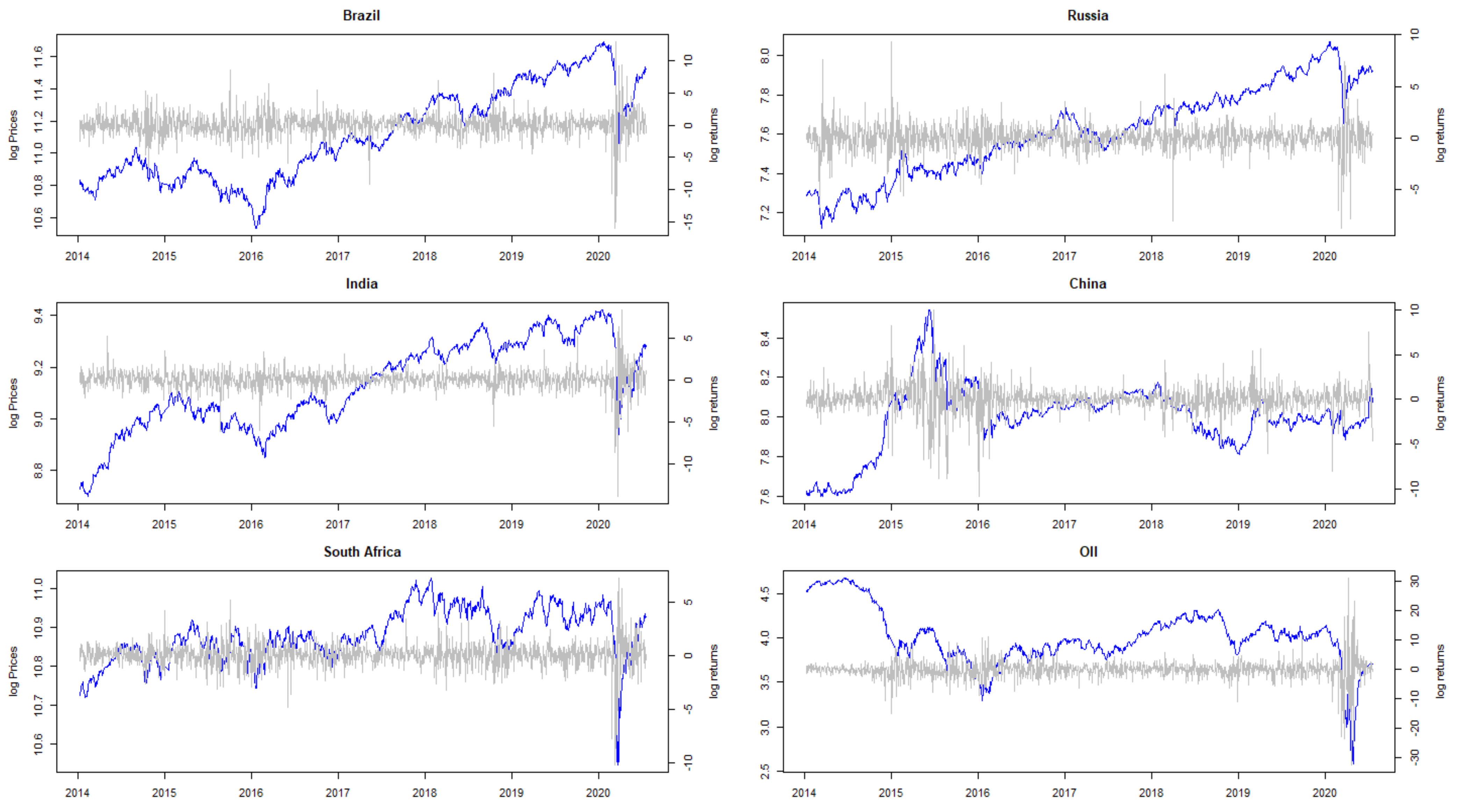
We used a data set consisting of daily stock prices, including stock indices for Brazil, Russia, India, China, South Africa, and crude oil, sourced from Yahoo finance and the Eikon Thomson Reuters database. The data samples ranged from 1 January 2014, to 17 July 2020, giving a total of 1300 daily observations for each asset. This sample period included the 2020 period featuring the current coronavirus-related stock and oil market crashes. Prices were converted to continuous compounded returns using the following relationship: $r_{i,t}=ln\frac{P_{i,t}}{P_{i,t-1}}\times 100,t=1,\cdots ,T=1300$, where $r_{i,t}$ is return of stock i and $P_{i,t}$ is the closing price of stock i at time t.

Table 1. Descriptive statistics.

	Brazil	Russia	India	China	South Africa	Crude Oil
Mean%	$0.0522$	$0.0487$	$0.0423$	$0.0346$	$0.0149$	$-0.0638$
Min%	$-15.99$	$-8.70$	$-13.90$	$-10.83$	$-10.23$	$-32.44$
Max%	$13.02$	$9.36$	$8.40$	$10.05$	$7.2610$	$31.33$
STD%	$1.9250$	$1.34$	$1.22$	$1.62$	$1.2220$	$3.48$
Ann SD	$30.43$	$21.31$	$19.44$	$25.61$	$19.33$	$55.08$
Kurtosis	$13.02$	$9.32$	$20.37$	$8.01$	$10.69$	$20.85$
Skewness	$-0.8886$	$-0.4062$	$-1.5740$	$-0.6850$	$-0.8625$	$-0.5184$
JB	9393	4764	23,120	3595	6377	23,700
$Q\left(10\right)$	$42.92$	$30.87$	$59.44$	$10.03$	$10.46$	$35.82$
$Q^2\left(10\right)$	$1251.0$	$316.5$	$798.5$	$298.9$	1374	1196
acf	$0.5520$	$0.2234$	$0.2038$	$0.2130$	$0.2731$	$0.3166$
Kendall’s Tau Correlation Matrix
Brazil	1	$0.223$	$0.124$	$0.072$	$0.212$	$0.217$
Russia	$0.223$	1	$0.202$	$0.116$	$0.317$	$0.177$
India	$0.124$	$0.202$	1	$0.140$	$0.286$	$0.044$
China	$0.072$	$0.116$	$0.140$	1	$0.195$	$0.056$
South Africa	$0.212$	$0.317$	$0.286$	$0.195$	1	$0.122$
Crude Oil	$0.217$	$0.177$	$0.044$	$0.056$	$0.122$	1

Notes: Both the Jarque–Bera (JB) test for normality and Box–Ljung (LJ) test for autocorrelation at lag 10, (Q(10 ), and squared returns $Q^2\left(10\right)$ test statistics were rejected at the 5% significance level. SD stands for standard deviation, Ann SD stands for annualized standard deviation, and acf represents the autocorrelation function at lag 1.

provides a summary of descriptive statistics based on continuous compounded returns. The sample means are all positive, except for crude oil (−0.0638%), and tall return series exhibit negative skewness and excess kurtosis, indicating a lack of symmetry in the underlying data distribution. This implies a higher probability of incurring extreme losses on the left tail during market downturns. This observation is supported by the small p-values < 5% significance level obtained from the Jarque–Bera test statistic, which leads us to reject the null hypothesis of normality. This indicates the presence asymmetry in asset returns and higher kurtosis in the tails more than the normal distribution (skewness = 0, kurtosis = 3). Our modeling strategy aims to account for this asymmetry by using a skewed Student’s t distribution for the innovations in our Markov-Switching GJR-GARCH modeling framework.

Figure 1 provides basic insight into the BRICS and world oil markets. They all provide further evidence of asymmetric behavior and dependence structures that need further investigation, through use of our proposed framework.

3.2. Estimation Results of VAR(2) Model

Table 2. Estimation results of VAR(2) model.

	Dependent Variable
	Brazil	Russia	India	China	South Africa	Crude Oil
${\mathrm{Brazil}}_{t-1}$	−0.084 ***	0.083 ***	0.092 ***	0.057	0.064 ***	−0.028
	(0.012)	(0.0003)	(0.00001)	(0.041)	(0.002)	(0.640)
${\mathrm{Russia}}_{t-1}$	0.033	−0.036	0.068 ***	−0.033	0.029	−0.043
	(0.484)	(0.284)	(0.023)	(0.414)	(0.322)	(0.620)
${\mathrm{India}}_{t-1}$	−0.112 ***	−0.124 ***	−0.093 ***	−0.041	−0.135 ***	0.061
	(0.037)	(0.001)	(0.005)	(0.358)	(0.00005)	(0.530)
${\mathrm{China}}_{t-1}$	−0.032	−0.021	−0.029	0.012	−0.037	−0.048
	(0.358)	(0.375)	(0.177)	(0.676)	(0.082)	(0.448)
${\mathrm{S}.\mathrm{Africa}}_{t-1}$	0.046	0.059	0.039	0.105 ***	0.005	0.066
	(0.442)	(0.152)	(0.289)	(0.035)	(0.902)	(0.541)
${\mathrm{Crude}.\mathrm{oil}}_{t-1}$	0.044 ***	0.035 ***	0.043 ***	0.038 ***	0.066 ***	−0.017
	(0.007)	(0.002)	(0.00003)	(0.006)	(0.000)	(0.564)
${\mathrm{Brazil}}_{t-2}$	−0.021	−0.001	0.041	0.016	0.043	0.066
	(0.526)	(0.980)	(0.047)	(0.578)	(0.040)	(0.283)
${\mathrm{Russia}}_{t-2}$	−0.040	0.008	−0.105 ***	0.011	−0.017	0.141
	(0.405)	(0.814)	(0.0004)	(0.783)	(0.563)	(0.107)
${\mathrm{India}}_{t-2}$	0.015	−0.038	0.005	0.005	0.033	−0.058
	(0.782)	(0.300)	(0.869)	(0.911)	(0.322)	(0.549)
${\mathrm{China}}_{t-2}$	−0.056	−0.013	−0.018	−0.005	−0.011	−0.036
	(0.107)	(0.595)	(0.392)	(0.864)	(0.595)	(0.564)
${\mathrm{S}.\mathrm{Africa}}_{t-2}$	0.105	0.131 ***	0.100 ***	0.048	0.015	0.136
	(0.075)	(0.001)	(0.006)	(0.336)	(0.684)	(0.205)
${\mathrm{Crude}.\mathrm{oil}}_{t-2}$	0.035	−0.029 **	−0.024	−0.035 ***	−0.003	−0.048
	(0.034)	(0.012)	(0.022)	(0.011)	(0.740)	(0.115)
Intercept	0.071	0.051	0.042	0.032	0.019	−0.073
	(0.182)	(0.165)	(0.203)	(0.481)	(0.560)	(0.451)

Notes: p-Values are reported in brackets. ** significant at 5% level; *** significant at 1% level. Portmanteau test: The null hypothesis of no autocorrelation was rejected, as the p-value of 0.000 < 0.05 was lower than the significance level.

reports the initial estimation from the vector autoregression VAR(2) model with lag length based on the BIC and AIC information criteria. The results show that the variables were bidirectional in some of the coefficients of the time-series, indicating a strong influence on current values of the dependent variables through lag 1 and lag 2 past values. In summary,

• Brazil’s current values were linearly dependent on lag 1 past values of Brazil, India, and crude oil, with p-values statistically significant at the 5% level.
• Russia’s current values were linearly dependent on lag 1 past values of Brazil, India, and crude oil and lag 2 values of Russia and South Africa, with p-values statistically significant at the 5% level.
• India’s current values were linearly dependent on lag 1 past values of Brazil, Russia, India, and crude oil as well as lag 2 values of Russia and South Africa, with p-values statistically significant at the 5% level.
• China’s current values were linearly dependent on lag 1 and lag 2 past values of crude oil, with p-values statistically significant at the 5% level.
• Crude Oil’s current values were not linearly dependent on the other BRICS stock returns, with p-values not statistically significant at the 5% level.

These results further highlight that the current BRICS returns are influenced by the past values of crude oil. These findings were also supported by the values of the correlation matrix on residuals, which motivates us to further investigate the overall dependence structure of crude oil with BRICS stock returns.

3.3. Results of Marginal Models Using MS-GJR-GARCH

Table 3. Parameter estimates of a two-state MS-GJR-GARCH(1,1) model with skewed Student’s t innovations.

	Brazil	Russia	India	China	South Africa	Crude Oil
	Regime 1
${\alpha }_{01}$	0.124 ***	0.016	0.008	0.012	0.026 ***	0.023 ***
	(0.002)	(0.094)	(0.188)	(0.024)	(0.001)	(0.000)
${\alpha }_{11}$	0.023	0.046	0.010	0.031	0.00000	0.00002 ***
	(0.141)	(0.102)	(0.201)	(0.081)	(0.493)	(0.000)
${\alpha }_{21}$	0.046	0.0001	0.006	0.019	0.105 ***	0.050 ***
	(0.085)	(0.481)	(0.387)	(0.265)	(0.0005)	(0.000)
${\beta }_1$	0.913 ***	0.931 ***	0.977 ***	0.950 ***	0.913 ***	0.966 ***
	(0.000)	(0.000)	(0.000)	(0.000)	(0.000)	(0.000)
${\nu }_1$	8.890 ***	99.800 ***	100.000 ***	3.670 ***	19.200 ***	5.550 ***
	(0.001)	(0.000)	(0.000)	(0.000)	(0.061)	(0.000)
${\xi }_1$	1.110 ***	0.436 ***	0.708 ***	1.010 ***	0.848 ***	0.869 ***
	(0.000)	(0.003)	(0.000)	(0.000)	(0.000)	(0.000)
	Regime 2
${\alpha }_{02}$	0.272 ***	0.110 **	0.059 **	3.580 ***	0.734 **	0.424 ***
	(0.001)	(0.050)	(0.029)	(0.003)	(0.358)	(0.000)
${\alpha }_{12}$	0.00000	0.0004	0.004	0.0001	0.0002	0.00002 ***
	(0.495)	(0.496)	(0.448)	(0.495)	(0.384)	(0.000)
${\alpha }_{22}$	0.246 ***	0.152${}^{*}$	0.470 ***	0.728 ***	0.056	0.385 ***
	(0.012)	(0.083)	(0.041)	(0.044)	(0.419)	(0.000)
${\beta }_2$	0.773 ***	0.870 ***	0.746 ***	0.312 ***	0.940 ***	0.807 ***
	(0.000)	(0.000)	(0.000)	(0.011)	(0.000)	(0.000)
${\nu }_2$	4.320 ***	3.710 ***	4.420 ***	5.300 ***	100.000 ***	99.800 ***
	(0.00000)	(0.00000)	(0.000)	(0.017)	(0.000)	(0.000)
${\xi }_2$	0.870 ***	1.110 ***	0.988 ***	0.866 ***	0.402 ***	0.994 ***
	(0.000)	(0.000)	(0.000)	(0.000)	(0.011)	(0.000)
	Transition probabilities
$p_{11}$	0.996 ***	0.424 ***	0.487 ***	0.996 ***	0.990 ***	0.992 ***
	(0.000)	(0.024)	(0.011)	(0.000)	(0.000)	(0.000)
$p_{21}$	0.005	0.399 ***	0.433 ***	0.021 ***	1.000 ***	0.027 ***
	(0.023)	(0.002)	(0.002)	(0.00000)	(0.091)	(0.000)
	Long run stable probabilities
Regime 1	$0.604$	$0.409$	$0.457$	$0.832$	$0.990$	$0.763$
Regime 2	$0.396$	$0.591$	$0.543$	$0.168$	$0.010$	$0.237$
	Unconditional volatility
Regime 1	26.91	13.03	13.52	17.83	14.78	30.24
Regime 2	26.93	20.77	21.11	53.65	85.66	110.1
	Volatility persistence
Regime 1	0.9590	0.9771	0.9900	0.9905	0.9655	0.9910
Regime 2	0.8960	0.9464	0.9850	0.6761	0.9682	0.9995
	Mean recurrence time (days)
Regime 1	$1.656$	$2.445$	$2.186$	$1.202$	$1.010$	$1.311$
Regime 2	$2.524$	$1.692$	$1.843$	$5.940$	$101.200$	$4.211$

Notes: p-Values are reported in brackets. ** significant at the 5% level. *** significant at the 1% level. Volatility persistence in the two regimes was calculated as ${\alpha }_{k;i,1}+\frac{1}{2}{\alpha }_{k;i,2}+{\beta }_{k;i}$, for regimes $k=1,2,i=1,2$. Unconditional variance in the two regimes was calculated as $\frac{{\alpha }_{k;0,i}}{\left[1-\left({\alpha }_{k;i,1}+\frac{1}{2}{\alpha }_{k;i,2}+{\beta }_{k;i}\right)\right]}$, for regimes $k=1,2;i=1,2$. The corresponding probabilities were computed as follows: $p_{22}=1-p_{21}$ and $p_{12}=1-p_{11}$.

presents in-sample parameter estimates for the MS-GJR-GARCH model with Skew Student’s t innovations and structural breaks (regime-switching). The table highlights interesting findings, where not all parameter estimates were statistically significant. The results also indicated that the evolution of the volatility process was not homogeneous across the two regimes. The estimated coefficient for the leverage effects, ${\alpha }_{2,i},i=1,2$, was not statistically significant in regime 1 for Brazil, Russia, India, and China. This indicates a lack of leverage effects, which implies the symmetric impact of bad news (negative news) and good news (positive news). Good news had an effect ${\alpha }_{1,i},i=1,2$, while bad news had an impact of ${\alpha }_{1,i}+{\alpha }_{2,i},i=1,2$. Furthermore, regime 1 was characterized by low unconditional volatility, while regime 2 was characterized by high unconditional volatility. The large degrees of freedom (${\nu }_1,{\nu }_2$) suggest that Russia, South Africa, and India could be modeled by normally distributed innovations.

Thus, each stock market can be summarized as follows:

• Brazil: Regime 1 was characterized by (i) lower unconditional volatility, (ii) low and non-significant reaction to past negative returns ${\alpha }_{21}\approx 0.046$, and (iii) higher persistence of the volatility process. Regime 2 was characterized by (i) higher unconditional volatility, (ii) high and statistically significant volatility reaction to past negative returns ${\alpha }_{22}\approx 0.246$, and (iii) lower persistence of the volatility process.
• Russia: Regime 1 was characterized by (i) low unconditional volatility, (ii) low and non-significant volatility reaction to past negative returns ${\alpha }_{21}\approx 0.001$, and (iii) high persistence of the volatility process. Regime 2 was characterized by (i) high unconditional volatility, (ii) high volatility reaction to past negative returns ${\alpha }_{22}\approx 0.152$, and (iii) low persistence of the volatility process.
• India: Regime 1 was characterized by (i) low unconditional volatility, (ii) low volatility reaction to past negative returns ${\alpha }_{21}\approx 0.006$, and (iii) high persistence of the volatility process. Regime 2 was characterized by (i) high unconditional volatility, (ii) high volatility reaction to past negative returns ${\alpha }_{22}\approx 0.470$, and (iii) high persistence of the volatility process.
• China: Regime 1 was characterized by (i) low unconditional volatility, (ii) weak and non-significant volatility reaction to past negative returns ${\alpha }_{21}\approx 0.019$, and (iii) high persistence of the volatility process. Regime 2 was characterized by (i) high unconditional volatility, (ii) high volatility reaction to past negative returns ${\alpha }_{22}\approx 0.728$, and (iii) low persistence of the volatility process.
• South Africa: Regime 1 was characterized by (i) low unconditional volatility, (ii) high and significant volatility reaction to past negative returns ${\alpha }_{21}\approx 0.105$, and (iii) low persistence of the volatility process. Regime 2 was characterized by (i) high unconditional volatility, (ii) low volatility reaction to past negative returns ${\alpha }_{22}\approx 0.056$, and (iii) high persistence of the volatility process.
• Crude oil: Regime 1 was characterized by (i) low unconditional volatility, (ii) low and non significant volatility reaction to past negative returns ${\alpha }_{21}\approx 0.050$, and (iii) low persistence of the volatility process. Regime 2 was characterized by (i) high unconditional volatility, (ii) high volatility reaction to past negative returns ${\alpha }_{22}\approx 0.385$, and (iii) high persistence of the volatility process.

The table also reports the long-run behavior Markov chain and the final matrix, which is called a stationary matrix, represented by long run stable probabilities. Clearly, for Brazil, the process stayed longer in regime 2 (≈1.7 days), Russia stayed longer in regime 1 (≈2.4 days), India stayed longer in regime 1 (≈2.2 days), China stayed longer in regime 2 (≈5.9 days), South Africa stayed longer in regime 2 (≈101.2 days), and Crude oil stayed longer in regime 2 (≈4.2 days). The average amount of time elapsed between visits to state i (called the mean recurrence time)2 was given by the reciprocal of the $i\mathrm{th}$ component of the long run stable probabilities (fixed probability vector).

3.4. Measuring Dependence with Vine Copula

In this section, we present the analytical estimates of the multivariate copula using regular vine (R-vine) and canonical vine (C-vine) models. Based on the AIC and BIC information criteria (C-vine: logLik: 646, AIC: −1245, BIC: −1126; R-vine: logLik: 643, AIC: −1244, BIC: −1136), we found that both models were adequate in capturing the dependence structure. However, the C-vine provided slightly better results, in comparison to the R-vine copula. Furthermore, for each variable pair, we first tested for the presence of an independent copula $C(u_1,u_2)=u_1.u_2$ and the small $p<0.05$ values leads us to reject the null hypothesis of independence and conclude that there exists pairwise dependence between the variable.

Table 4. Results of C-vine copulas, with Kendall’s tau and upper/lower tail dependences.

	Copula C(.)	Edge ${\mathit{E}}_{\mathit{i}}$	Parameter 1 ${\mathit{\theta }}_1$	Parameter 2 ${\mathit{\theta }}_2$	Tau $\mathit{\tau }$	Lower Tail ${\mathit{\lambda }}_{\mathit{l}}$	Upper Tail ${\mathit{\lambda }}_{\mathit{u}}$
Tree 1	t	5,4	0.293 ***	16.600 **	0.189	0.006	0.006
			(0.026)	(8.200)
	t	5,3	0.430 ***	7.900 ***	0.283	0.093	0.093
			(0.023)	(1.820)
	t	5,2	0.455 ***	7.700 ***	0.301	0.106	0.106
			(0.023)	(1.690)
	BB1	5,1	0.328 ***	1.100 ***	0.220	0.146	0.123
			(0.053)	(0.029)
	SBB7	6,5	1.150 ***	0.125 ***	0.129	0.174	0.004
			(0.030)	(0.037)
Tree 2	I	1,4|5	0.000	0.000	0.000	0.000	0.000
	t	1,3|5	0.109 ***	15.000 **	0.070	0.002	0.002
			(0.029)	(6.080)
	t	1,2|5	0.241 ***	9.470 ***	0.155	0.029	0.029
			(0.028)	(2.970)
	F	6,1|5	1.570 ***	0.000	0.167	0.000	0.000
			(0.171)
Tree 3	I	2,4|1,5	0.000	0.000	0.000	0.000	0.000
	t	2,3|1,5	0.103 ***	14.300 ***	0.066	0.003	0.003
			(0.029)	(5.300)
	BB8	6,2|1,5	1.450 ***	0.794 ***	0.093	0.000	0.000
			(0.299)	(0.180)
Tree 4	t	3,4|2,1,5	0.088 ***	11.400 ***	0.056	0.007	0.007
			(0.030)	(3.930)
	BB7-90	6,3|2,1,5	−1.030 ***	−0.067 **	−0.048	0.000	0.000
			(0.018)	(0.033)
Tree 5	I	6,4,|3,2,1,5	0.000	0.000	0.000	0.000	0.000

Notes: p-Values are reported in brackets. ** significant at the 5% level. *** significant at the 1% level. I: = Independent copula; t: = t copula; BB1: = Clayton–Gumbel; SBB7: = Joe–Clayton copula; BB8: = Frank–Joe; BB7-90: = rotated Joe–Clayton copula (90 degrees). node 1 = Brazil, node 2 = Russia, node 3 = India, node 4 = China, node 5 = South Africa, node 6 = crude oil.

shows the parameter estimates for the proposed 6-dimensional C-vine pairwise dependence among the variables, together with detailed information on the number of tree sequences, the family of the fitted bivariate copula ($C(.)$, Kendall’s tau ($\tau$), and lower ${\lambda }_l$ and upper ${\lambda }_u$ tail dependence probabilities.

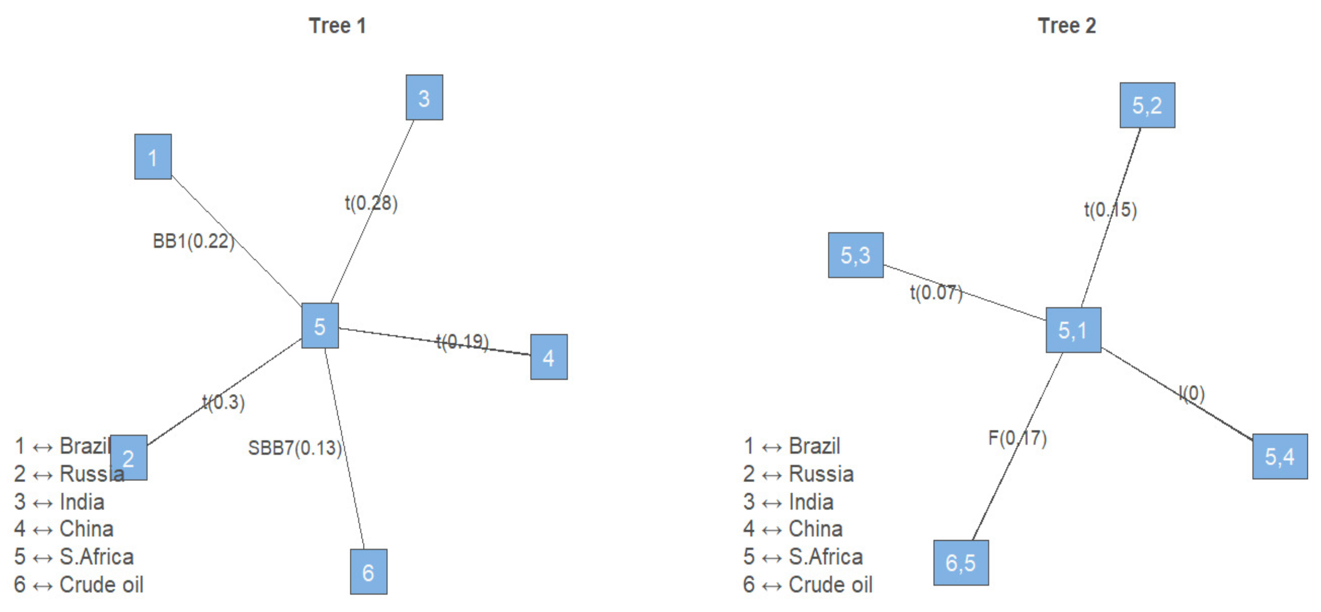
Figure 2 displays the corresponding Tree 1 and Tree 2 for the C-vine, where the nodes represent random variables (assets); thus, node 1: = Brazil, node 2: = Russia, node 3: = India, node 4: = China, node 5: = South Africa, and node 6: = crude oil. The corresponding edges represent the type and best family copula, fitted with values shown in brackets, which measure the strength of the dependence structure based on the Kendall’s tau rank-based correlation.

As can be seen from the plots, South Africa (represented by node 5) was selected as the center root node, as it showed stronger dependence with the other five assets. The pairwise empirical Kendall’s $\tau$ values ranged from $0.130$ to $0.301$. We found two types of tail dependence structure: symmetric tail dependence between South Africa and China, South Africa and Russia, and South Africa and India; and asymmetric lower tail dependence between South Africa and Brazil, as well as South Africa and crude oil. However, the dependence in Trees 2–5 were relatively small, preventing us from drawing any meaningful conclusions. The information about the lower tail probability found between South Africa and Brazil (14.6%) and the South Africa and crude oil (17.4%) markets are important indicators for investors, as they may help investors to diversify their portfolios during times of financial distress.

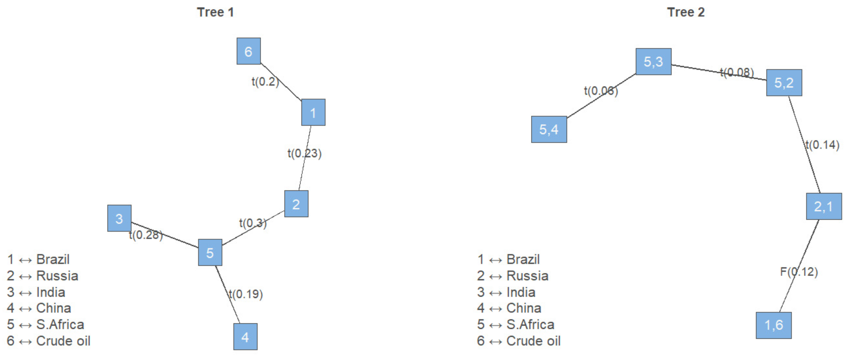
The R-vine copula results are reported in

Table 5. Results of R-vine copulas, with Kendall’s tau and upper/lower tail dependences.

	Copula C(.)	Edge ${\mathit{E}}_{\mathit{i}}$	Parameter 1 ${\mathit{\theta }}_1$	Parameter 2 ${\mathit{\theta }}_2$	Tau $\mathit{\tau }$	Lower Tail ${\mathit{\lambda }}_{\mathit{l}}$	Upper Tail ${\mathit{\lambda }}_{\mathit{u}}$
Tree 1	t	1,6	0.307 ***	10.500 ***	0.199	0.030	0.030
			(0.026)	(3.250)
	t	2,1	0.358 ***	5.420 ***	0.233	0.129	0.129
			(0.026)	(1.020)
	t	5,2	0.455 ***	7.700 ***	0.301	0.106	0.106
			(0.023)	(1.690)
	t	5,3	0.430 ***	7.900 ***	0.283	0.093	0.093
			(0.023)	(1.820)
	t	5,4	0.293 ***	16.600 **	0.189	0.006	0.006
			(0.026)	(8.200)
Tree 2	F	2,6|1	1.060 ***	0.000	0.116	0.000	0.000
			(0.167)
	t	5,1|2	0.215 ***	11.000 ***	0.138	0.017	0.017
			(0.028)	(3.640)
	t	3,2|5	0.124 ***	12.400 ***	0.079	0.006	0.006
			(0.029)	(4.230)
	t	4,3|5	0.096 ***	8.470 ***	0.061	0.020	0.020
			(0.030)	(2.250)
Tree 3	I	5,6|2,1	0.000	0.000	0.000	0.000	0.000
Tree 3	I	3,1|5,2	0.087 ***	16.700 **	0.055	0.001	0.001
			(0.029)	(7.380)
	t	4,2|3,5	0.000	0.000	0.000	0.000	0.000
Tree 4	BB7-90	3,6|5,2,1	−1.030 ***	−0.066 **	−0.047	0.000	0.000
			(0.018)	(0.032)
	I	4,1|3,5,2	0.000	0.000	0.000	0.000	0.000
Tree 5	I	4,6|3,5,2,1	0.000	0.000	0.000	0.000	0.000

Notes: p-Values are reported in brackets. ** significant at the 5% level. *** significant at the 1% level. I: = Independent copula; t: = t copula; F: = Frank copulas; BB7-90: = rotated Joe–Clayton copula. node 1 = Brazil, node 2 = Russia, node 3 = India, node 4 = China, node 5 = South Africa, node 6 = crude oil.

. The dependence was captured using the bivariate elliptical Student’s t copula, with which exhibited symmetric tail dependence between Brazil and crude oil, Brazil and Russia, South Africa and Russia, South Africa and India, and South Africa and China. The dependences in Trees 2–5 were too small to draw any meaningful conclusions. Figure 3 shows the corresponding dependence trees in graphical format.

3.5. Market Risk under Portfolio Rebalancing

In this section, the above results were applied to a portfolio optimization problem and the model performance was compared, based on four data sets: (i) the data with returns that did not account for switching and dependence, (ii) returns with switching but no dependence, (iii) returns with switching and C-vine dependence, and (iv) returns with switching and R-vine dependence. Markowitz’s mean variance portfolio Markowitz (1959), which focuses on the variance risk measure, has been criticized by finance practitioners as it penalizes extreme tail losses. This problem has been addressed by using alternative risk measures, such as Value-at-Risk (VaR) and Conditional Value-at-Risk (CVaR) is a coherent risk measure proposed by Rockafellar and Uryasev (2000), which has now replaced $\mathrm{VaR}$ in BCBS (2019) under the revised market risk models. Here, we propose an asset allocation model for a portfolio that minimizes 95% of portfolio Conditional Value-at-Risk as the objective function.

Let $w=(w_1,w_2,w_3,w_4,w_5,w_6)$ be the portfolio weights vector representing the number of stocks held in asset $i,(i=1,\cdots ,6)$. Thus, $w_i$ are decision (optimization) variable and, $r=(r_1,\cdots ,r_6)$ denote a random vector of asset returns with a multivariate probability density function denoted by $p\left(r\right|w)$. Let the one dimensional loss function $\xi =f(w,r)$ be a random variable observed over time. Then, the cumulative distribution function of the loss for the return vector given a threshold value ${\xi }_0$ can be written in integral form as follows,

$$\begin{array}{c}\hfill \mathsf{\Psi }(w,\xi )={\int }_{f(w,r)\le {\xi }_0}p\left(r\right|w)dr=Pr\left(\xi \le {\xi }_0\right)\end{array}$$

(10)

Then, for a given confidence level $\alpha$, $\mathrm{VaR}{}_{\alpha }$ is the $\alpha$-quantile of a loss distribution associated with portfolio which can be represented as,

$$\begin{array}{c}\hfill \mathrm{VaR}{}_{\alpha }\left(\xi \right)=\inf \left(\xi \in \mathbb{R}\left|\mathsf{\Psi }\right(w,\xi )\ge \alpha \right)\end{array}$$

(11)

However, $\mathrm{VaR}$ measure does not take into account losses beyond the threshold ${\xi }_0$ and it is nonconvex and not subadditive like $\mathrm{CVaR}$ see, Fabozzi et al. (2007).

Accordingly, the investor whose focus is in the lower tail dependence, solves the minimization of the $\mathrm{CVaR}$ for the portfolio excess loss function as follows,

$$\begin{array}{cccc}\hfill & \underset{\mathbf{w}}{\mathrm{minimize}}\hfill & \hfill {\mathrm{CVaR}}_{\alpha }\left(\xi \right)& =\mathbb{E}\left[\xi |\xi >Va{R}_{\alpha }\left(\xi \right)\right]\hfill \\ \hfill & \hfill & \hfill \sum _{i=1}^d{w}_i& =1\hfill \\ \hfill & \hfill & \hfill w_i& \ge 0,i=1,\cdots ,6\hfill \end{array},$$

(12)

where $\mathbb{E}\left[\xi |\xi >Va{R}_{\alpha }\left(\xi \right)\right]=\frac{1}{1-\alpha }{\int }_{{}_{f(w,r)\ge Va{R}_{\alpha }\left(\xi \right)}}f(w,r)p\left(r\right|w)dr$, and $Va{R}_{\alpha }\left(\xi \right)$ is defined as the smallest number ${\xi }_0$ such that the probability of a negative loss ${\xi }_0$ is not higher than the ($1-\alpha$) quantile of the distribution set at $\alpha =95\%$. We assume no short-selling portfolio (long portfolio) thus, $w_i\ge 0$ are non-negative portfolio weights and ${\sum }_{i=1}^6{w}_i=1$ is the capital budget constraint.

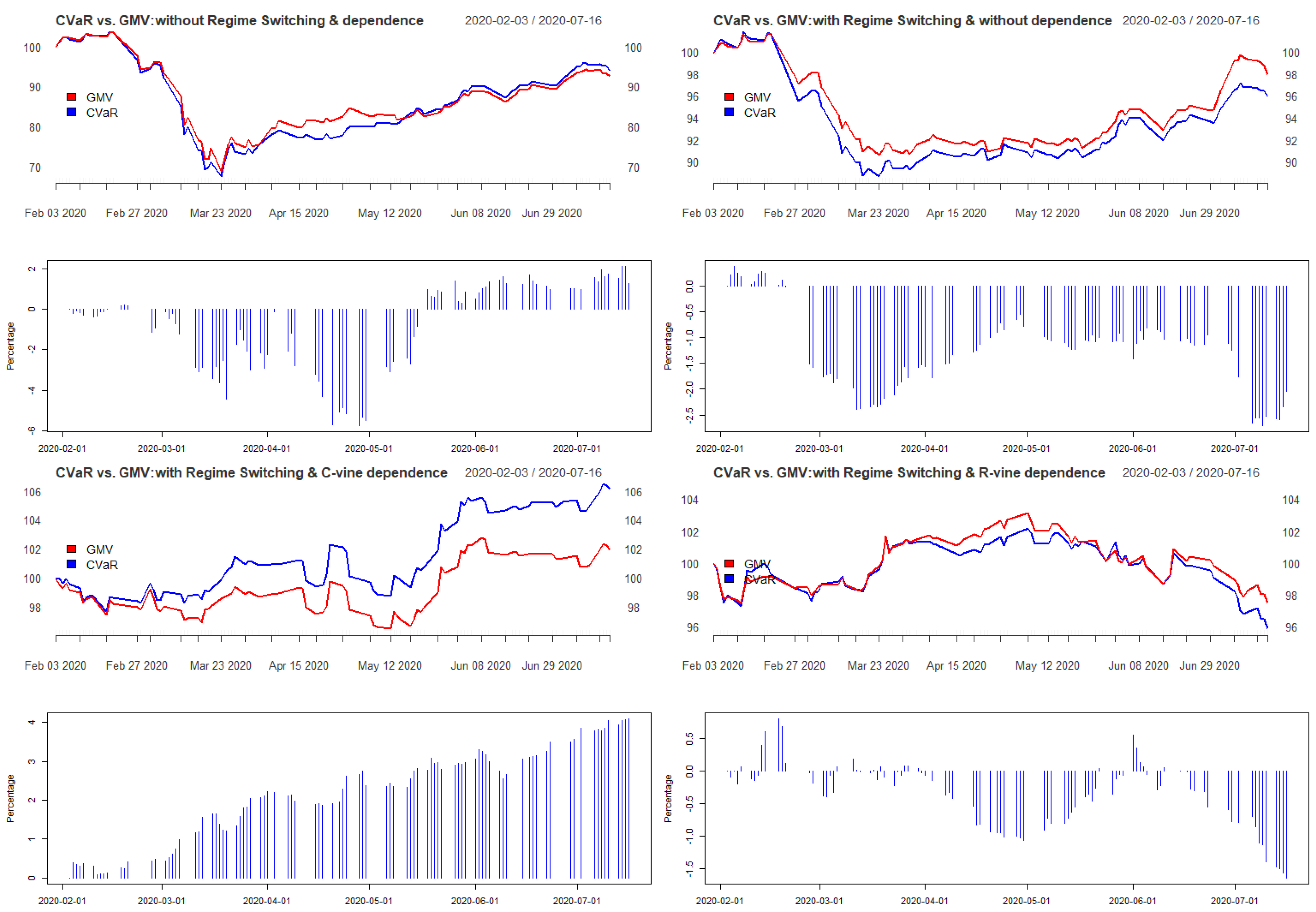
Figure 4 displays four equity plots, highlighting the in-sample relative performance of minimum CVaR, compared with the mean variance (MV) portfolio (also known as the global minimum variance portfolio). The MV finds a trade-off between the expected return, $\mathbb{E}\left(r\right)$, and the risk of the portfolio, measured by the variance $w^T\mathsf{\Sigma }w$. The performance measurement was based on a starting capital allocation of 100 with a rebalancing strategy. The C-vine portfolio strategy clearly outperformed all other portfolio constructions: Thus, it outperformed the portfolio without regime-switching and without dependence, the portfolio with a two state regime-switching but without dependence, and the R-vine portfolio. We argue that a C-vine portfolio construction strategy can adequately model the portfolio risk and account for the asset dependence structure and draw-downs observed during the COVID-19 financial market crisis in 2020.

Table 6. Risk and weight allocation without regime-switching and dependence.

Period	Cvar	Brazil	Russia	India	China	South Africa	Crude Oil
1	$0.01900$	$0.14545$	$0.15776$	$0.18743$	$0.12297$	$0.20197$	$0.18442$
2	$0.02088$	$0.13791$	$0.16760$	$0.16398$	$0.14302$	$0.20625$	$0.18123$
3	$0.02785$	$0.16968$	$0.16417$	$0.16575$	$0.16574$	$0.20288$	$0.13177$
4	$0.03043$	$0.13701$	$0.21248$	$0.14158$	$0.16319$	$0.15157$	$0.19417$
5	$0.03061$	$0.10606$	$0.19845$	$0.13964$	$0.15770$	$0.17669$	$0.22147$
6	$0.02924$	$0.15521$	$0.18522$	$0.14004$	$0.20150$	$0.17874$	$0.13928$
7	$0.02798$	$0.16008$	$0.19691$	$0.10827$	$0.16227$	$0.20428$	$0.16819$

,

Table 7. Risk and weight allocation with regime-switching and without dependence.

Period	Cvar	Brazil	Russia	India	China	South Africa	Crude Oil
1	$0.01380$	$0.16264$	$0.17232$	$0.17319$	$0.13308$	$0.19422$	$0.16456$
2	$0.01504$	$0.16869$	$0.16766$	$0.17844$	$0.13099$	$0.17722$	$0.17701$
3	$0.01561$	$0.17285$	$0.16899$	$0.17977$	$0.12241$	$0.17540$	$0.18058$
4	$0.01558$	$0.17413$	$0.16835$	$0.17943$	$0.12225$	$0.17490$	$0.18094$
5	$0.01551$	$0.17417$	$0.16790$	$0.18037$	$0.12211$	$0.17475$	$0.18070$
6	$0.01548$	$0.17370$	$0.16785$	$0.18024$	$0.12263$	$0.17488$	$0.18070$
7	$0.01542$	$0.17271$	$0.16791$	$0.18086$	$0.12291$	$0.17543$	$0.18019$

,

Table 8. Risk and weight allocation with regime-switching and C-vine dependence.

Period	Cvar	Brazil	Russia	India	China	South Africa	Crude Oil
1	$0.01060$	$0.18690$	$0.18879$	$0.14672$	$0.13690$	$0.19998$	$0.14071$
2	$0.01060$	$0.18687$	$0.18650$	$0.14343$	$0.13857$	$0.20132$	$0.14331$
3	$0.01058$	$0.18724$	$0.18578$	$0.14385$	$0.13941$	$0.20130$	$0.14242$
4	$0.01070$	$0.19441$	$0.18951$	$0.14296$	$0.13371$	$0.20086$	$0.13856$
5	$0.01061$	$0.14386$	$0.20222$	$0.15399$	$0.16276$	$0.19128$	$0.14589$
6	$0.01037$	$0.15062$	$0.14601$	$0.15646$	$0.17047$	$0.16127$	$0.21516$
7	$0.01060$	$0.19368$	$0.19135$	$0.14334$	$0.13373$	$0.19860$	$0.13931$

and

Table 9. Risk and weight allocation with regime-switching and R-vine dependence.

Period	Cvar	Brazil	Russia	India	China	South Africa	Crude Oil
1	$0.01019$	$0.19888$	$0.19317$	$0.14236$	$0.12400$	$0.18836$	$0.15323$
2	$0.01024$	$0.19718$	$0.19220$	$0.14472$	$0.12159$	$0.18990$	$0.15441$
3	$0.01023$	$0.19634$	$0.19209$	$0.14445$	$0.12188$	$0.19030$	$0.15494$
4	$0.01019$	$0.19646$	$0.19255$	$0.14343$	$0.12192$	$0.18959$	$0.15604$
5	$0.01015$	$0.19591$	$0.19213$	$0.14433$	$0.12259$	$0.18945$	$0.15560$
6	$0.01018$	$0.19518$	$0.19383$	$0.14415$	$0.12121$	$0.19012$	$0.15551$
7	$0.01017$	$0.19608$	$0.19366$	$0.14450$	$0.12074$	$0.19066$	$0.15437$

report the estimated minimum CVaR portfolios with percentage marginal contribution of each return series under a rebalancing framework. It is evident that the C-vine and R-vine portfolios contributed the lowest aggregated risk. We argue that portfolio construction that takes into account both regime-switching and the dependence structure can yield optimal risk diversification. Overall, the C-vine portfolio had the best performance over the rebalancing period, as depicted in Figure 4, when compared to a benchmark global minimum variance (GMV) portfolio.

Figure 4 displays the four return trajectory plots, together with bar plots (blue) showing the relative performance between the CVaR versus a benchmark GMV portfolio. The C-vine portfolio strategy with re-balancing strategy clearly outperformed both the MS-GJR-GARCH without dependence and the benchmark portfolio with no regime-switching and no dependence. Therefore, the extreme portfolio draw-downs observed during the COVID-19 financial market crisis in 2020 could be adequately captured.

4. Conclusions

In this study, we attempted to analyze the tail dependence structure in BRICS and crude oil markets, as well as to determine optimal investment decisions in these markets, by using a combination of different statistical techniques, including vector autoregression (VAR2), Markov-switching GJR-GARCH, vine copula, and particle swarm optimization techniques. First, the returns series for the indices were pre-filtered using VAR(2) to model the conditional mean and to account for the linear influence of lag 1 and lag 2 of other variables. Second, a Markov-switching Garch (MS-GJR-GARCH) volatility process was adopted, in order to remove the effects of autocorrelation and to account for heteroscedasticity, leveraging effects and regime-switching parameters. The results of modeling the volatility process showed evidence of two separate regimes, indicated by the in-homogenous (different) unconditional volatility. We also found high volatility persistence across all return series, in both regime 1 and regime 2, with the exception of China in regime 2; as well as high persistence in transition probability between the two regimes. That is, the Markov chain showed the propensity to stay equally as long in both regimes, as indicated by the high probabilities of staying in regime 1 and regime 2.

On the other hand, the results of modeling the dependence structure using the Pairwise Copula Construction (PCC) with vine copula provided more insight into the complex relationships among the returns. This multivariate copula approach was adopted to account for different dependence structures between asset returns in the BRICS and crude oil markets. Based on the Akaike Information criteria (AIC), we found that the C-vine copula model was adequate in describing the complex relationships.

As a result, we found two types of tail dependence structures: symmetric tail dependence, captured by an elliptical Student’s t copula, between South Africa and China, South Africa and Russia, and South Africa and India; and asymmetric lower tail dependence between South Africa and Brazil, as well as South Africa and crude oil. Therefore, we argue that information about the lower tail probability found between South Africa and Brazil (14.6%) or South Africa and crude oil (17.4%) markets are important indicators for investors, which may help investors to diversify their portfolios during times of financial distress. However, the dependence in exhibited in Trees 3–5 were negligible, preventing us from drawing any meaningful inferences. In addition, the symmetric tail dependence coefficients are also vital, which may help investors to diversify or hedge their portfolios during times of financial distresses.

To determine optimal investment strategies in these markets, we made use of the estimated C-vine and R-vine copulas, in order to simulate returns, and applied the Particle Swam optimization technique to the quantile-transformed innovations, in order to determine the overall minimum CVaR and the corresponding marginal risk contributions of each asset return. The Particle Swam was metaheuristic, requiring few assumptions about the problem being optimized and providing greater flexibility due to being a derivative-free optimization algorithm. It is a naturally inspired technique that finds the optimal solution iteratively, by trying to improve the candidate solution and avoiding sub-optimal investment solutions.

The optimization results under a rebalancing strategy confirmed the existence an inverse relationship between the risk contribution and asset allocation of South Africa and oil, supporting the existence of a higher lower tail dependence between them. We argue that, when the South African stock market is in distress, investors tend to shift their holdings in oil market. Similar results were found between Brazil and crude oil. Furthermore, we found that the rebalancing strategy which accounts for regime-switching and the dependence structure outperformed all other portfolio strategies, including a portfolio without regime-switching and dependency or a portfolio with only regime-switching. In the symmetric tail, South African asset allocation was found to have well-diversified relationships with those of China, Russia, and India, suggesting that these three markets might be good investment destinations when things are not good in South Africa, and vice versa.

These findings are vital for international investors, policymakers, and regulators during both bull and bear markets. However, the limitation of this model is its inability to account for other hidden stylized facts, such as price jumps and long-memory processes in stock returns. in future research, we will try to account for these factors.

References

1. Aas, Kjersti, and Daniel Berg. 2009. Models for construction of multivariate dependence—A comparison study. The European Journal of Finance 15: 639–59. [Google Scholar] [CrossRef]
2. Aas, Kjersti, Claudia Czado, Arnoldo Frigessi, and Henrik Bakken. 2009. Pair-copula constructions of multiple dependence. Insurance: Mathematics and Economics 44: 182–98. [Google Scholar] [CrossRef] [Green Version]
3. Apergis, Nicholas, and Stephen M. Miller. 2009. Do structural oil-market shocks affect stock prices? Energy Economics 31: 569–75. [Google Scholar] [CrossRef] [Green Version]
4. Ardia, David, Keven Bluteau, Kris Boudt, and Leopoldo Catania. 2018. Forecasting risk with markov-switching garch models: A large-scale performance study. International Journal of Forecasting 34: 733–47. [Google Scholar] [CrossRef]
5. Ardia, David, Keven Bluteau, Kris Boudt, Leopoldo Catania, and Denis-Alexandre Trottier. 2019. Markov-switching garch models in r: The msgarch package. Journal of Statistical Software 91. [Google Scholar] [CrossRef] [Green Version]
6. BCBS. 2019. Minimum Capital Requirements for Market Risk. BASEL III. Available online: https://www.bis.org/bcbs/publ/d457.pdf (accessed on 30 March 2021).
7. Bedford, Tim, and Roger M. Cooke. 2001. Probability density decomposition for conditionally dependent random variables modeled by vines. Annals of Mathematics and Artificial Intelligence 32: 245–68. [Google Scholar] [CrossRef]
8. Bedford, Tim, and Roger M. Cooke. 2002. Vines: A new graphical model for dependent random variables. Annals of Statistics 30: 1031–68. [Google Scholar] [CrossRef]
9. Bekiros, Stelios, Jose Arreola Hernandez, Shawkat Hammoudeh, and Duc Khuong Nguyen. 2015. Multivariate dependence risk and portfolio optimization: An application to mining stock portfolios. Resources Policy 46: 1–11. [Google Scholar] [CrossRef]
10. BenSaïda, Ahmed. 2018. The contagion effect in european sovereign debt markets: A regime-switching vine copula approach. International Review of Financial Analysis 58: 153–65. [Google Scholar] [CrossRef]
11. Bhar, Ramaprasad, and Biljana Nikolova. 2009. Return, volatility spillovers and dynamic correlation in the bric equity markets: An analysis using a bivariate egarch framework. Global Finance Journal 19: 203–18. [Google Scholar] [CrossRef]
12. Bollerslev, Tim. 1990. Modelling the coherence in short-run nominal exchange rates: A multivariate generalized arch model. The Review of Economics and Statistics 72: 498–505. [Google Scholar] [CrossRef]
13. Bonga-Bonga, Lumengo. 2018. Uncovering equity market contagion among brics countries: An application of the multivariate garch model. The Quarterly Review of Economics and Finance 67: 36–44. [Google Scholar] [CrossRef] [Green Version]
14. Bouri, Elie, Syed Jawad Hussain Shahzad, Naveed Raza, and David Roubaud. 2018. Oil volatility and sovereign risk of brics. Energy Economics 70: 258–69. [Google Scholar] [CrossRef]
15. BoussaïD, Ilhem, Julien Lepagnot, and Patrick Siarry. 2013. A survey on optimization metaheuristics. Information Sciences 237: 82–117. [Google Scholar] [CrossRef]
16. Brechmann, Eike Christain, and Claudia Czado. 2013. Risk management with high-dimensional vine copulas: An analysis of the euro stoxx 50. Statistics and Risk Modeling 30: 307–42. [Google Scholar] [CrossRef]
17. Cherubini, Umberto, Elisa Luciano, and Walter Vecchiato. 2004. Copula Methods in Finance. West Sussex: John Wiley & Sons. [Google Scholar]
18. Chkili, Walid, and Duc Khuong Nguyen. 2014. Exchange rate movements and stock market returns in a regime-switching environment: Evidence for brics countries. Research in International Business and Finance 31: 46–56. [Google Scholar] [CrossRef]
19. Czado, Claudia. 2019. Analyzing dependent data with vine copulas. In Lecture Notes in Statistics. Basel: Springer. [Google Scholar]
20. de Melo Mendes, Beatriz Vaz, and Daniel S. Marques. 2012. Choosing an optimal investment strategy: The role of robust pair-copulas based portfolios. Emerging Markets Review 13: 449–64. [Google Scholar] [CrossRef]
21. Engel, Robert F. 1990. Discussion: Stock market volatility and the crash. Review of Financial Studies 3: 103–6. [Google Scholar] [CrossRef]
22. Engle, Robert F. 2002. A simple class of multivariate generalized autoregressive conditional heteroskedasticity models. Journal of Business and Economics Statistcs 20: 339–50. [Google Scholar] [CrossRef]
23. Engle, Robert, and Bryan Kelly. 2012. Dynamic equicorrelation. Journal of Business & Economic Statistics 30: 212–28. [Google Scholar]
24. Fabozzi, Frank J., Petter N. Kolm, Dessislava A. Pachamanova, and Sergio M. Focardi. 2007. Robust Portfolio Optimization and Management. Hoboken: John Wiley & Sons. [Google Scholar]
25. Gatfaoui, Hayette. 2019. Diversifying portfolios of us stocks with crude oil and natural gas: A regime-dependent optimization with several risk measures. Energy Economics 80: 132–52. [Google Scholar] [CrossRef] [Green Version]
26. Glosten, Lawrence R., Ravi Jagannathan, and David E. Runkle. 1993. On the relation between the expected value and the volatility of the nominal excess return on stocks. The Journal of Finance 48: 1779–801. [Google Scholar] [CrossRef]
27. Haas, Markus, Stefan Mittnik, and Marc S. Paolella. 2004. A new approach to markov-switching garch models. Journal of Financial Econometrics 2: 493–530. [Google Scholar] [CrossRef]
28. Hansen, Bruce E. 1994. Autoregressive conditional density estimation. International Economic Review 35: 705–30. [Google Scholar] [CrossRef]
29. Hassan, Kamrul, Ariful Hoque, Muammer Wali, and Dominic Gasbarro. 2020. Islamic stocks, conventional stocks, and crude oil: Directional volatility spillover analysis in brics. Energy Economics 92: 104985. [Google Scholar] [CrossRef]
30. Hernandez, Jose Arreola. 2014. Are oil and gas stocks from the australian market riskier than coal and uranium stocks? dependence risk analysis and portfolio optimization. Energy Economics 45: 528–36. [Google Scholar] [CrossRef]
31. Hou, Yang, Steven Li, and Fenghua Wen. 2019. Time-varying volatility spillover between chinese fuel oil and stock index futures markets based on a dcc-garch model with a semi-nonparametric approach. Energy Economics 83: 119–43. [Google Scholar] [CrossRef]
32. Jaworski, Piotr, Fabrizio Durante, Wolfgang Karl Hardle, and Tomasz Rychlik. 2010. Copula Theory and Its Applications. London: Springer, vol. 198. [Google Scholar]
33. Ji, Qiang, Bing-Yue Liu, Wan-Li Zhao, and Ying Fan. 2018. Modelling dynamic dependence and risk spillover between all oil price shocks and stock market returns in the brics. International Review of Financial Analysis 68: 101238. [Google Scholar] [CrossRef]
34. Jiang, Yonghong, Yuyuan Fu, and Weihua Ruan. 2019. Risk spillovers and portfolio management between precious metal and brics stock markets. Physica A: Statistical Mechanics and its Applications 534: 120993. [Google Scholar] [CrossRef]
35. Joe, Harry. 1996. Families of m-variate distributions with given margins and m (m-1)/2 bivariate dependence parameters. Lecture Notes-Monograph Series 28: 120–41. [Google Scholar]
36. Junker, Markus, and Angelika May. 2005. Measurement of aggregate risk with copulas. The Econometrics Journal 8: 428–54. [Google Scholar] [CrossRef]
37. Kenourgios, Dimitris, Aristeidis Samitas, and Nikos Paltalidis. 2011. Financial crises and stock market contagion in a multivariate time-varying asymmetric framework. Journal of International Financial Markets, Institutions and Money 21: 92–106. [Google Scholar] [CrossRef]
38. Kocaarslan, Baris, Ramazan Sari, Alper Gormus, and Ugur Soytas. 2017. Dynamic correlations between bric and us stock markets: The asymmetric impact of volatility expectations in oil, gold and financial markets. Journal of Commodity Markets 7: 41–56. [Google Scholar] [CrossRef]
39. Kole, Erik, Kees Koedijk, and Marno Verbeek. 2007. Selecting copulas for risk management. Journal of Banking & Finance 31: 2405–23. [Google Scholar]
40. Kumar, Satish, Aviral Kumar Tiwari, Yogesh Chauhan, and Qiang Ji. 2019. Dependence structure between the brics foreign exchange and stock markets using the dependence-switching copula approach. International Review of Financial Analysis 63: 273–84. [Google Scholar] [CrossRef]
41. Lambert, Philippe, and Sébastien Laurent. 2001. Modelling Skewness Dynamics in Series of Financial Data Using Skewed Location-Scale Distributions. Discussion Paper No. 01-25, Institut de Statistique, Université Catholique de Louvain, Louvain-la-Neuve, Belgium. Available online: http://www.statsoc.ulg.ac.be/workingpapers_pl.html (accessed on 30 March 2021).
42. Lin, Ling, Zhongbao Zhou, Yong Jiang, and Yangchen Ou. 2021. Risk spillovers and hedge strategies between global crude oil markets and stock markets: Do regime switching processes combining long memory and asymmetry matter? The North American Journal of Economics and Finance 57: 101398. [Google Scholar] [CrossRef]
43. Low, Rand Kwong Yew, Jamie Alcock, Robert Faff, and Timothy Brailsford. 2013. Canonical vine copulas in the context of modern portfolio management: Are they worth it? Journal of Banking & Finance 37: 3085–99. [Google Scholar]
44. Markowitz, Harry. 1959. Portfolio Selection. New Haven: Yale University Press. [Google Scholar]
45. Mba, Jules Clement, and Sutene Mwambi. 2020. A markov-switching cogarch approach to cryptocurrency portfolio selection and optimization. Financial Markets and Portfolio Management 34: 199–214. [Google Scholar] [CrossRef]
46. McIver, Ron P., and Sang Hoon Kang. 2020. Financial crises and the dynamics of the spillovers between the us and brics stock markets. Research in International Business and Finance 54: 101276. [Google Scholar] [CrossRef]
47. Mensi, Walid, Shawkat Hammoudeh, Duc Khuong Nguyen, and Sang Hoon Kang. 2016. Global financial crisis and spillover effects among the us and brics stock markets. International Review of Economics & Finance 42: 257–76. [Google Scholar]
48. Morema, Kgotso, and Lumengo Bonga-Bonga. 2020. The impact of oil and gold price fluctuations on the south african equity market: Volatility spillovers and financial policy implications. Resources Policy 68: 101740. [Google Scholar] [CrossRef]
49. Nelsen, Roger B. 2007. An Introduction to Copulas. New York: Springer Science & Business Media. [Google Scholar]
50. Nelson, Daniel B. 1991. Conditional heteroskedasticity in asset returns: A new approach. Econometrica: Journal of the Econometric Society 59: 347–70. [Google Scholar] [CrossRef]
51. Nguyen, Cuong C., and M. Ishaq Bhatti. 2012. Copula model dependency between oil prices and stock markets: Evidence from china and vietnam. Journal of International Financial Markets, Institutions and Money 22: 758–73. [Google Scholar] [CrossRef]
52. Peng, Xiaofan. 2020. Do precious metals act as hedges or safe havens for china’s financial markets? Finance Research Letters 37: 101353. [Google Scholar] [CrossRef]
53. Rockafellar, R. Tyrrell, and Stanislav Uryasev. 2000. Optimization of conditional value-at-risk. Journal of Risk 2: 21–42. [Google Scholar] [CrossRef] [Green Version]
54. Sahamkhadam, Maziar, Andreas Stephan, and Ralf Östermark. 2018. Portfolio optimization based on garch-evt-copula forecasting models. International Journal of Forecasting 34: 497–506. [Google Scholar] [CrossRef]
55. Salisu, Afees A., and Rangan Gupta. 2020. Oil shocks and stock market volatility of the brics: A garch-midas approach. Global Finance Journal 48: 100546. [Google Scholar] [CrossRef]
56. Sensoy, Ahmet, Erk Hacihasanoglu, and Duc Khuong Nguyen. 2015. Dynamic convergence of commodity futures: Not all types of commodities are alike. Resources Policy 44: 150–60. [Google Scholar] [CrossRef] [Green Version]
57. Sklar, A. 1959. Fonctions de repartition an dimensions et leurs marges. Publications de l’Institut Statistique de l’Université de Paris 8: 229–31. [Google Scholar]
58. Sui, Lu, and Lijuan Sun. 2016. Spillover effects between exchange rates and stock prices: Evidence from brics around the recent global financial crisis. Research in International Business and Finance 36: 459–71. [Google Scholar] [CrossRef]
59. Thampanya, Natthinee, Muhammad Ali Nasir, and Toan Luu Duc Huynh. 2020. Asymmetric correlation and hedging effectiveness of gold & cryptocurrencies: From pre-industrial to the 4th industrial revolution. Technological Forecasting and Social Change 159: 120195. [Google Scholar]
60. Trottier, Denis-Alexandre, and David Ardia. 2016. Moments of standardized fernandez–steel skewed distributions: Applications to the estimation of garch-type models. Finance Research Letters 18: 311–16. [Google Scholar] [CrossRef]
61. Umar, Zaghum. 2017. The demand of energy from an optimal portfolio choice perspective. Economic Modelling 61: 478–94. [Google Scholar] [CrossRef]
62. Weiß, Gregor N. F. 2013. Copula-garch versus dynamic conditional correlation: An empirical study on var and es forecasting accuracy. Review of Quantitative Finance and Accounting 41: 179–202. [Google Scholar] [CrossRef]
63. Zakoian, Jean-Michel. 1994. Threshold heteroskedastic models. Journal of Economic Dynamics and control 18: 931–55. [Google Scholar] [CrossRef]
Figure 1. Actual historical closing log-prices and log-returns of BRICS and crude oil from January 2014 to July 2020.
Ijfs 09 00030 g001
Figure 2. Results of C-vine copula dependency, showing trees 1 and 2, with nodes (variables) and edges (Kendall’s Tau).
Ijfs 09 00030 g002
Figure 3. Results of R-vine copulas dependency showing trees 1 and 2, with nodes (variables) and edges (Kendall’s Tau).
Ijfs 09 00030 g003
Figure 4. Trajectory of Minimum CVaR vs. Global Minimum Variance (GMV) rebalancing portfolio performance.
Ijfs 09 00030 g004