
The Effect of Quantitative Easing through Google Metrics on US Stock Indices


1
Department of Economics, University of Thessaly, 28th October Str. 78, 38333 Volos, Greece
2
Department of Social Science, Hellenic Open University, Parodos Aristotelous Str. 18, 26335 Patras, Greece
*
Author to whom correspondence should be addressed.
Int. J. Financial Stud. 2021, 9(4), 56; https://0-doi-org.brum.beds.ac.uk/10.3390/ijfs9040056
Submission received: 9 August 2021
/
Revised: 23 September 2021
/
Accepted: 24 September 2021
/
Published: 3 October 2021
Abstract
:The purpose of this study is to investigate the fluctuations that occur in stock returns of US stock indices when there is an increase in the volume of Google internet searches for the phrase “quantitative easing” in the US. The exponential generalized autoregressive conditional heteroscedasticity model (EGARCH) was applied based on weekly data of stock indices using the three-factor model of Fama and French for the period of 1 January 2006 to 30 October 2020. The existence of a statistically significant relationship between searches and financial variables, especially in the stock market, is evident. The result is strong in three of the four stock indices studied. Specifically, the SVI index was statistically significant, with a positive trend for the S&P 500 and Dow Jones indices and a negative trend for the VIX index. Investor focus on quantitative easing (QE), as determined by Google metrics, seems to calm stock market volatility and increase stock returns. Although there is a large body of research using Google Trends as a crowdsourcing method of forecasting stock returns, this paper is the first to examine the relationship between the increase in internet searches of “quantitative easing” and stock market returns.
1. Introduction
Central banks pursue monetary policy by changing the money supply, credit, and interest rates for economic prosperity. They use daily monetary policy transmission tools, which are categorized as either conventional or nonconventional. Under normal circumstances, the central bank is not involved in direct lending to the private sector or government, or in indirect purchases of government bonds, corporate debt, or other types of debt instruments. The recent financial crisis has forced central banks to address a series of problems that the conventional methods which have been applied for so many years could not solve. The Great Recession of 2007–2009 pushed short-term interest rates to almost 0%, i.e., below the central bank threshold. The need to apply nonconventional monetary instruments to ease the economic downturn then became apparent. Distinguished among nonconventional monetary policy measures is the large-scale asset purchasing policy (LSAP), or quantitative easing (QE), as applied by the Federal Reserve and the BoE since late 2008 and early 2009.
The benefits of quantitative easing are generally well understood by professionals and academics. Through QE, monetary authorities hope to encourage affected economies by reducing yields, thereby reducing the cost of capital for businesses and households; as such, consumption and investment spending are expected to increase. The goal of QE is to contribute money to the economy in order to stimulate nominal spending. When the monetary authority buys these assets by creating new money or reserves for commercial banks, it also increases the number of deposits held by the nonbanking private sector, which includes households and businesses. Various transmission channels have been identified through which the purchase of assets could affect aggregate demand. Weale and Wieladek (2016) discussed three mechanisms: the expectation management channel, the portfolio balancing channel, and the signaling channel. The Deutsche Bundesbank (2016) identified two additional channels: the balance sheet channel, and the exchange rate channel. An interesting question that has been raised over recent years is the role of the stock market in the economy and these channels, and whether these excess reserves contributed to the significant stock market boom.
Knowledge of stock market behavior in response to macroeconomic change is essential for policymakers and those seeking return on investment. Several studies have been conducted to analyze the effect of quantitative easing in multiple contexts (Papadamou et al. 2020b), such as how quickly one can distinguish it from the moment it is announced by the competent body, and then whether an investor can maximize profits by anticipating the corresponding public reaction. Typically, research in this area reveals statistics to support the theory that monetary policy affects the stock market (Ioannidis and Kontonikas 2008; Gregoriou et al. 2009; Apergis 2019; Bauer and Rudebusch 2014). Our study, using crowdsourcing data based on Google searches, investigates responses of US stock index returns and implied volatility on QE policy via an asset pricing framework.
We argue that the existence of a correlation between the data of search queries via internet and financial variables, especially in the stock market, is evident from previous studies (Vlastakis and Markellos 2012; Da et al. 2011). The majority of these studies were focused on search metrics concerning earning or other news about a specific stock company. However, this effect was not strong in all cases. As investors pay close attention to stocks, they are able to immediately incorporate new information into stock prices, which leads to higher yield volatility. Due to higher volatility, investors require higher returns to hedge the increased risk. Another study that provided empirical evidence of a positive correlation between stock market volatility and Google search metrics focused on investor attention on the COVID-19 pandemic (Papadamou et al. 2020a). The goal of the present paper is to evaluate the effectiveness of Google Trends data as a measure of investor market attention regarding unconventional monetary policy measures and not firm specific news.
Our paper contributes to this growing body of literature about investor attention based on Google metrics, stock returns, and volatility by highlighting the effects of quantitative easing policies. Previous studies focused on the announcement of QE by central banks and its effects on the macroeconomy (for a survey, see Papadamou et al. 2020b), but not on investor attention based on Google metrics. Our focus is on the popular stock market indicators Nasdaq, S&P 500, Dow Jones, and VIX. The main research hypotheses are the following: (a) stock market index returns are positively correlated with increased investor attention, as determined using Google metrics, on QE policy; and (b) stock market volatility is calmed when investor attention on quantitative easing increases. Our findings indicate that investor attention on QE seems to calm stock market volatility and increase stock returns.
2. Relevant Literature
One of the main functions of financial markets is to channel capital into productive activities, which requires resources in the economy. This simple transfer promotes the development of the national economy, competitiveness, and employment. For this transfer of resources to be effective, investors and investees transmit and request information about these investments. One of the main themes of the financial literature is to understand how this information affects stakeholders and, consequently, the prices of assets in financial markets (Fama 1970). Understanding information has become a challenge for research, given the lack of data on investor behavior and the decision-making process. Given the developments in the field of information technology, using crowdsourcing as a practice of obtaining information, or opinions from a large group of people who submit their data via the internet, has become prevalent. Therefore, the acquisition of data in search queries by popular search engines, such as Google, is available. At present, it is possible to export a time series of search query data for the term “stock market”, for example.
The Google search engine is by far the most popular and widely used data collection platform in the world, collecting 90% of the searches performed worldwide. Google also monitors statistics for various search queries made on its platform, and these are made available to the public through Google Trends. Since its inception in 2004, Google Trends has become the tool of choice for most researchers worldwide. Google collects billions of data every day, in which one enters a query in a box. Aggregate data can be useful to shed light on some research questions and are available for free for the first time. Explicitly, the types of searches performed by users will be an honest indicator of the interests, issues, or intentions of the general public; however, these searches do not essentially represent the views of users. In addition, users search when they want to find more information, indicating that the results may favor recent events or issues in the audience.
The information provided by the platform has attracted the attention of the research community and has been used either to identify trends or to predict the dynamics, among others, of the stock market. For example, a significant increase in the search volume for the influenza epidemic may indicate the onset of an outbreak in a specific area (Ginsberg et al. 2009). Similarly, there may be an increase in online queries for certain types of cars, predicting future sales (Kristoufek 2013). The traditional view of financial markets presupposes its effectiveness and that all relevant information is incorporated into the existing share price (Fama 1970). However, recent technological advances in the digital age have led to the transition from traditional theory to information-based digital economics. This economic change has prompted further research by scholars who deny market effectiveness, with measurable indicators of investor attention. In finance, Google search query data may indicate an individual’s bias in trading in financial markets or the systematic increase in investor attention (Da et al. 2011). Both results can be indicators of an investor’s future behavior. The increase in searches for the term “stock market” can be understood as a predictor of a systematic increase in the market by investors and an increase in stock prices. The use of these signals that precede financial market behavior is relevant, as it can be useful to build portfolios, predict a financial crisis, and, in general, understand the factors that affect the prices of financial agreements. The research of Papadamou et al. (2021) studied the impact of the recent COVID-19 pandemic, based on the time-varying correlation between stock returns and bonds. Using the SVI index, for the specific term coronavirus, but also the general issue, they found that the correlation between stocks and bonds was affected by the recent pandemic, as government bonds showed an upward trend due to investors’ preference for government bonds.
Several studies aimed to forecast short-term economic indicators based on data from Google Trends. Examples include car sales, unemployment rates, consumer confidence, inflation, and outbreaks. The study by Ettredge and Karuga (2005) pioneered the use of Google Trends data to support macroeconomic data analysis and forecasting. The authors analyzed the unemployment time series in the United States and concluded that the Google Trends series were related to unemployment during the 77 weeks of the sample. In this way, this type of approach is proposed as it can help predict macroeconomic variables. Choi and Varian (2012) tested the predictive power of data from Google Trends on consumption metrics, unemployment insurance benefits, and consumer confidence. Using simple econometric models, the authors showed that estimates using Google Trends data exceeded twenty percent more predictability than estimates based on different datasets. Several researchers have also investigated the effect of Google search queries on market volatility and examined their predictive power. Predicting market volatility is important for financial investment decisions. Volatility reflects the magnitude of the risk associated with a stock or index. Therefore, in order to evaluate a particular financial product, an investor must make some predictions about future volatility. It is therefore desirable to predict variability as accurately as possible. Increasing investor interest can increase market volatility, meaning it can be a useful predictor of volatility.
Vlastakis and Markellos (2012) studied the demand and supply of information for stocks and found that the demand for information at the market level is positively correlated with historical and indicated instability. They used the keyword search volume associated with 30 of the largest stocks traded on the NYSE, Nasdaq, and S&P 500. They commented that the differences in the demand for information have a significant effect on each stock and the overall level of the market, in terms of historical volatility and trading volume. They ended up accepting the hypothesis that describes an increase in the demand for information at the same time as an increase in the level of risk aversion in the market. Da et al. (2011), using data from Russel 3000 shares from 2004 to 2008, showed that an increase in the SVI (Google search volume index) predicted higher stock prices over the next 2 weeks, and then prices returned within the year. They also showed that the SVI captures the attention of investors in a timelier manner, compared to other indicators, and that this attention is mainly from retail investors. Preis et al. (2013) found patterns that can be read as alerts from financial transactions on the stock market. Using a sample of data from 2004 to 2011, their results showed that Google Trends data not only reflect real stock market behavior but can also predict future trends. Their study concluded that the platform data can be used to build profitable strategies. Bijl et al. (2016) found that company name query data can be used to predict weekly stock returns for individual companies, with their results showing that a high search volume predicted low future returns. However, the relationship between performance and search volume was weak but robust and statistically significant. A trading strategy based on their findings also yielded low profitability due to high transaction costs. Papadamou et al. (2020a) investigated the effect of an increased search volume on the global SARS-CoV-2 coronavirus epidemic on the volatility of thirteen major stock exchanges, covering Europe, Asia, the USA, and Australia. They found the existence of a positive relationship between them, that is, with the increase in the volume of searches, the variability increases at the same time, indicating the presence of a channel of transmission of risk aversion to investors. Stock market volatility was directly affected, and stock yields were indirectly reduced. They also noted that the impact was stronger in Europe, compared to other continents.
Investors are worried about volatility forecasts to create their best portfolios. When constructing an investment portfolio, various methods can be used to determine the weighting of each stock in the portfolio, based on expected return and risk. Investment strategies have been widely discussed in the academic literature, and the use of Google Trends data could make a significant contribution to achieving higher returns. Kristoufek (2013) created portfolios with adjustable weights, based on the search query volumes from Google Trends, and showed that the portfolios formed under this strategy show lower volatility than the equally weighted portfolios. In this way, these studies approach the effective market hypothesis: if there is any information that can help predict stock returns and is not embedded in asset prices (in our case, online search information for financial assets), one can consider this fact as a rejection of the effective market assumption.
3. Data and Methodology
3.1. Stock Indices
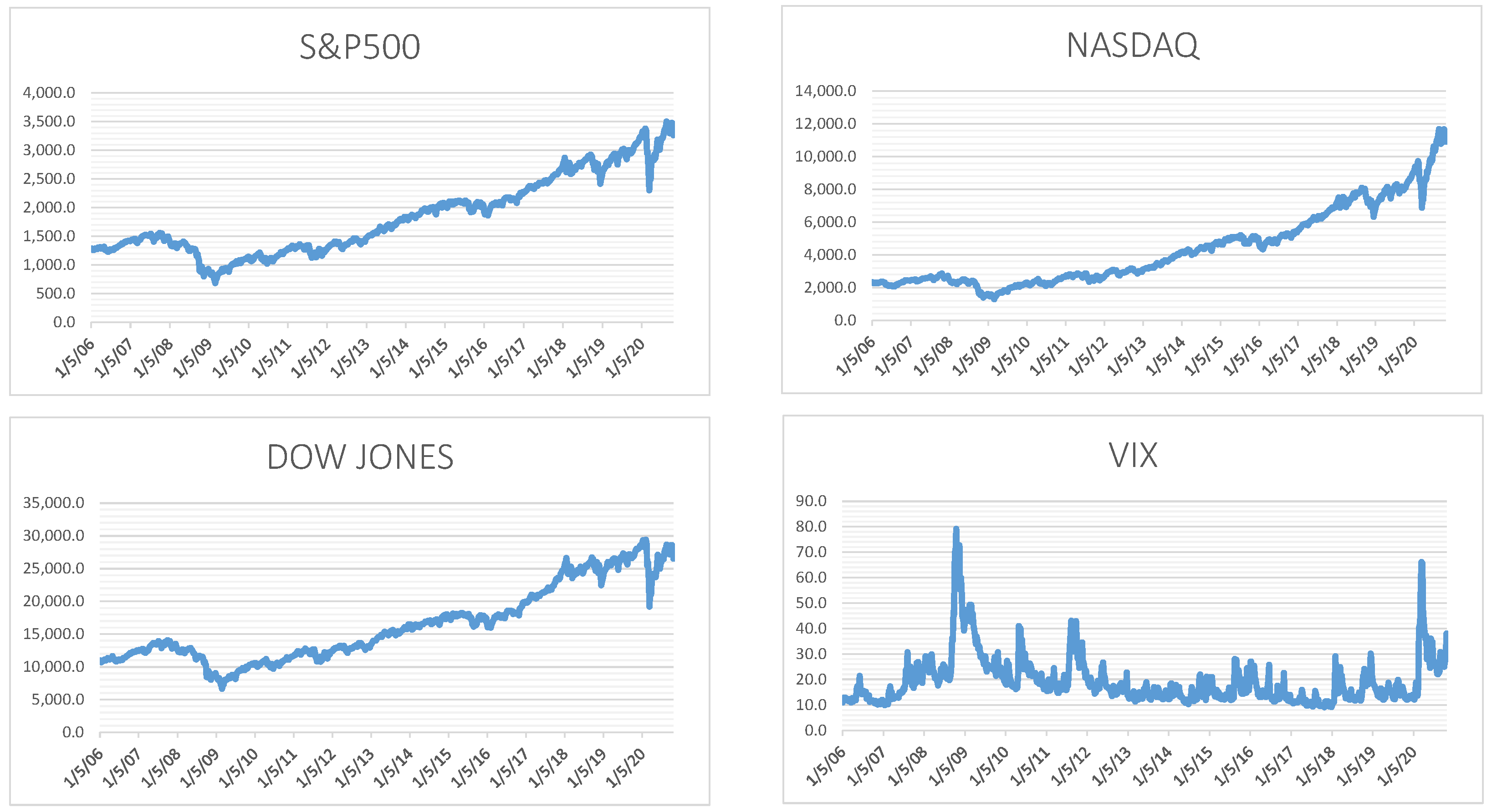
The dataset used in the present study consists of the stock indices Nasdaq, S&P 500, Dow Jones, and VIX, with data taken from the Yahoo Finance website. Prices were taken on a weekly basis to match the results of the Google search volume. For the analysis performed, the set of variables includes only quantitative data. The date of 1 January 2006 was chosen as the starting point because the Google Trends platform does not provide data earlier than that. The year 2006 was chosen to avoid the recession after the bubble in the early 2000s. The final date was chosen to be 30 October 2020 because the prices of the three factors published by Fama and French were calculated by then. Table 1 presents the descriptive statistics of the data, in terms of their weekly returns, which resulted from the closing prices, and Figure 1 represents the evolution of the returns of the stock indices during the examined period. In summary, the prices of the stock indices of the analysis have an upward trend within the period under study, which is shown by their positive, on average, weekly returns. The VIX index shows the highest average performance, followed by the Nasdaq index. Fluctuation measures the variability of observations around the mean value.
The Dow Jones index shows the smallest fluctuation; therefore, it is considered the safest, compared to the rest, while having the lowest yield. During the 774 weeks examined, the Dow Jones, Nasdaq, and S&P 500 indices showed the lowest performance on 6 October 2008, with −18.1%, −15.2%, and −18.2%, respectively. The three stock indices show low negative asymmetry, showing that most returns are higher than expected, while in the case of the VIX index, where positive asymmetry is recorded, the opposite is true. The indices of the analysis show a kurtosis higher than 3, indicating the high frequency of extreme values. In particular, the VIX index shows the highest curvature, with a value of 13.3, and then the Dow Jones index with a value of 13.24.
3.2. Google Trends
By entering a search term/word and a specified geographic location, the site provides information about the frequency of queries to the search engine related to the specified term or word. If there is a sufficient amount of data, the tool provides weekly or monthly information. The data are normalized in such a way that they are in the range between 0 and 100. To achieve this relative frequency, each nominal value for a given period is divided by the maximum value over the same period (Choi and Varian 2012). The platform calculates the volume of searches for each word based on all its uses. For example, search query data for the word “quantitative easing” will also include search queries for “quantitative easing and stocks”, and “what is quantitative easing”, among other queries. Frequently asked questions by the same users are not included in the price calculation. Google Trends results come in the form of relative search frequencies or search volume indices (SVIs) from absolute search frequencies, possibly for privacy reasons. Specifically,
where the SVI of a current search word t is an integer between 0 and 100 and is calculated as the search volume V(t) of the word at that time t, divided by the maximum search volume V(max) of that word, over a time period Δt.
SVI = V(i,t)/V(max,Δt)
The weekly data from Google Trends, calculated from Saturday to Sunday, are published on Monday and are available for any time period between 2004 and 2016. On the other hand, daily data are only possible for periods not exceeding three months. However, the Google Trends tool allows you to add up to 5 different time ranges, all of which are standardized by the same formula with a unique range.
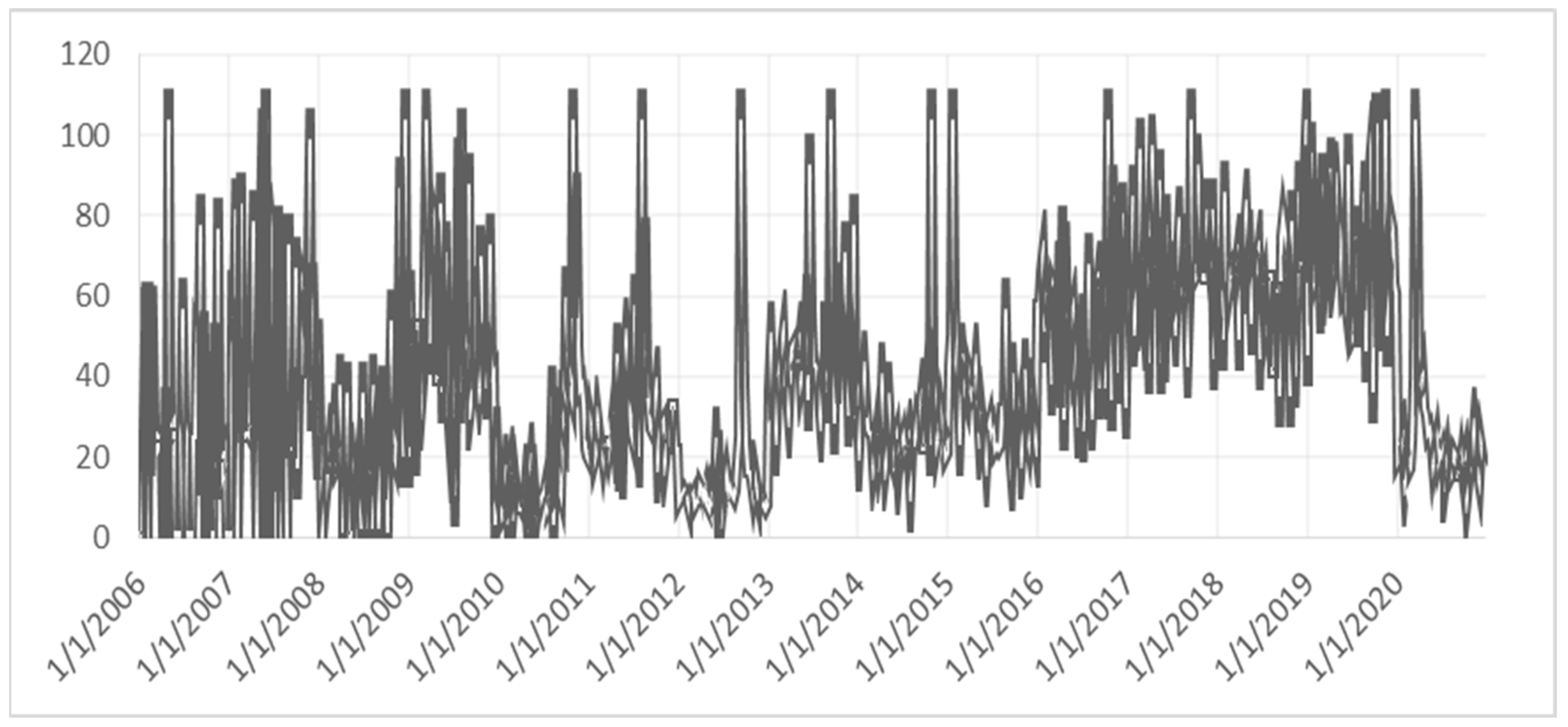
Figure 2 presents the data provided by the platform, meaning the search queries for “Quantitative Easing”, on a weekly basis, from 2006 to 2020. From January 2006 to September 2008, low values of the index are observed, indicating low interest in the issue. Then, a steady increase follows, where in September 2009, it peaks with the data up to that point. Then, in the following months, the upward trend of the index continues until September 2012, when it reaches the maximum value of 100 points. It is worth noting that the above data concern the geographical area of the USA. At the same time, the Federal Reserve launched a quantitative easing program. We can highlight that the increase in the volume of Google internet searches also depends on media coverage of the news. According to Akhtaruzzaman et al. (2021), media coverage can facilitate transmitting a contagion across markets.
3.3. Methodology
The analysis period starts on 6 January 2006 and ends on 30 October 2020, with a weekly frequency of 774 weeks. This study is based on the weekly closing prices of the stock indices as well as the weekly prices of the indices of the number of searches. Each observation of the stock indices and the index of the number of searches was calculated from the Friday of the previous period (t − 1) until the next (t). The logarithmic differences in the weekly observations were then calculated, resulting in 774 observations for each time series. Finally, the data based on which the empirical results of the study were extracted consisted of a set of 8 time series.
The topic of quantitative easing in internet searches was chosen instead of a specific query, or search term, because web search data related to specific search terms may be incomplete. There are several different search terms by which a user can search for information on the topic of interest; thus, choosing the general topic of quantitative easing covers the full range of queries, or search terms.
The stock returns were modeled in an asset pricing framework, following the Fama–French three-factor model, while conditional volatility of returns was estimated with an EGARCH model, as in the study of Papadamou and Siriopoulos (2014). The reliable Fama–French asset pricing model consists of three explanatory variables, namely, the excess market return to risk-free interest rate, SMB (small capitalization minus large), and HML (high book value to market minus low). All the data were collected from the Kenneth R. French online data library. Specifically, the model was constructed as follows:
where Rt is the return on the stock index in week t, β0 is the fixed term, β1 is the coefficient market risk factor, β2 is the coefficient of small capitalization minus large, β3 is the coefficient of high book value to market minus low, β5 is the coefficient of the volume of internet searches with one lag, and β6 is the coefficient with two lags. The main hypothesis that was checked is whether the volume of internet searches on quantitative easing is related to the trend of stock index returns, that is, whether changes in the search volume cause changes in index yields. The control of the case was based on the three-factor model, asset pricing, of Fama and French, following the methodology of exponential-type GARCH. The variability is described as follows:
where the error term is based on the generalized error distribution (hereinafter “GED”), and the queue parameter is k > 0. The GED is a symmetric family of distributions used in mathematical modeling, usually when the errors (the difference between the expected value and the observed values) are not normally distributed. Three parameters determine the distribution: First, there is the average, which determines the mode (the top) of the distribution. As in a normal distribution, the median is equal to m. Second, there is the standard deviation, σ, that determines the dispersion. Third, the shape parameter, K, refers to kurtosis and follows a normal distribution if k = 2, and with fat tails if k < 2.
Rt = β0 + β1 (rm − rf) + β2 (SMBt) + β3 (HMLt) + β4 (SVIt) + β5 (SVI(t−1)) + β6 (SVI(t−2)) + et
ln(σ2(j,t)) = ω + βln(σ2(j,t−1)) + γ ε(j,t−1)/√(σ2(j,t−1)) + α1| ε(j,t−1)/√(σ2(j,t−1))| + α2 |ε (j,t−2)/√(σ2(j,t−2))|
ε(j,t)|Ω(t−1)~GED(0,σ2(j,t),k)
The asymmetric EGARCH model has two advantages over the conventional GARCH. First, the logarithmic construction of Equation (3) ensures that the estimated conditional variance is strictly positive, and thus the non-negative constraints used to estimate the ARCH and GARCH models are not necessary. Second, asymmetries are allowed, i.e., if the relationship between volatility and returns is negative, γ will be negative. Therefore, the presence of the known leverage effect in the financial literature (i.e., the fact that multiple significant falls in returns are associated with increased volatility) can be controlled by the hypothesis, if it is negative. The effect is asymmetric if γ ≠ 0.
We used the Akaike, Schwarz, and Hannan–Quinn criteria to evaluate the different p and q parameters and concluded that the EGARCH (2,1) was the best, given it had the lowest results. Continuing, we implemented three unit root tests to deduct whether the time series were stationary or not. The tests used were the augmented Dickey–Fuller, Phillips–Perron, and Kwiatkowski–Phillips–Schmidt–Shin tests, which indicated all the time series were integrated of order 1; therefore, first differences were implemented. We then conducted the ARCH test to examine the possibility of an ARCH effect in our data. The results indicated no ARCH effect on the residues.
4. Empirical Results
Before looking at the results, we must point out that the EGARCH models were evaluated with different classes of parameters p and q, where the selection of the most suitable model for each model was conducted by evaluating the Akaike, Schwarz, and Hannan–Quinn criteria. The selection was based on the lowest value of the criteria. For each model evaluated, the criteria were minimized with the EGARCH model (2,1), as shown in Table 2.
It should be mentioned that unit root tests were conducted in order to assess whether any of the time series are stationary. The tests used were the augmented Dickey–Fuller, Phillips–Perron, and Kwiatkowski–Phillips–Schmidt–Shin tests. The augmented Dickey–Fuller and Phillips–Perron tests have H0 as their initial hypothesis, the hypothesis of the existence of a unit root, as opposed to the alternative Ha, hypothesizing the existence of a stationary chronological order. The Kwiatkowski–Phillips–Schmidt–Shin test has H0 as its initial hypothesis, the stationarity hypothesis, compared to the alternative Ha, concerning the existence of a unit root. Based on the results shown in Table 3, all the time series were integrated of order 1; therefore, first differences were implemented.
Continuing, the ARCH test for the EGARCH model (2,1) was performed in order to verify the incorporation of nonlinearity by the model. The hypothesis was checked with either the F or the LM statistic NR2, which is distributed as an χ2 distribution with p degrees of freedom. If NR2 <χ2 or if F <Fα, the null hypothesis is not rejected, and this means that there is no ARCH result, and homoscedasticity applies. If rejected, there is an ARCH effect, and heteroscedasticity. The results are presented below. From Table 4, it is understood that the problem of nonlinearity in the variance was solved, since the probability is higher for all indices. Therefore, for each level of statistical significance, the null hypothesis that there is no ARCH effect on the residues is accepted.
The maximum likelihood estimates of the three-factor Fama–French model are presented in Table 5 in order to reveal the effect of the SVI on stock index returns. In general, from Table 5, it is concluded that the market index coefficient (β1) is statistically significant and positive. In addition, in terms of the SMB and HML ratios, they are statistically significant for each stock index. In particular, they seem to have a negative effect on the performance of the S&P 500; SMB positively affects and HML negatively affects the performance of the Nasdaq; and the opposite is true for the Dow Jones index. Additionally, the SVI index is statistically significant for the S&P 500 and Dow Jones indices and has a positive effect. Therefore, the first hypothesis of our study, regarding the positive correlation between stock market indices’ returns and increased investor attention via Google metrics on QE policy, is correct.
That is, if the volume of searches on quantitative easing increases by 1%, the returns will increase by 0.000563 and 0.003053 points for the S&P 500 and Dow Jones indices, respectively. This result is in line with the conclusion of Papadamou et al. (2020a), who found a positive relationship between QE and stock and bond prices. In contrast, in the case of the Nasdaq index, it does not appear to have a statistically significant effect on its performance. Therefore, investors in the traditional S&P 500 and Dow Jones stock indices are more prone to QE announcements than investors in the Nasdaq technology index. This is in line with the point made by Ajayi et al. (2006) about the difference between the behavior of large-cap stock trading dominated by institutional investors and small-cap stock trading dominated by individual investors. They showed that that post-event market volatility is significantly higher in the periods following unfavorable events compared to the volatility following favorable events for the NYSE, S&P 500, and DJIA indices, but in the case of indices consisting of small-cap companies and individual investors such as RUSSEL 2000 and Nasdaq, the post-event market volatility is higher following unexpected favorable events than for periods following unfavorable events.
In no stock index is the volume of searches of the previous week or the previous two weeks statistically significant, apart from the VIX index. In the case of the VIX index, the volume of searches of the previous two weeks is the only one that is statistically significant. Therefore, the volume of internet searches, two weeks ago, seems to affect the returns of the VIX index, reducing them by 0.000465. Consequently, the second hypothesis of our study, concerning the calmed effect on stock market volatility when investor attention on quantitative easing is expanded, is also correct. This is in line with Fassas and Papadamou’s (2018) research entitled “Unconventional monetary policy announcements and risk aversion: evidence from the U.S. and European equity markets”. The researchers found that in the days leading up to the federal announcement of the QE program, there was a decline in the VIX index.
The last part of the table presents some diagnostic tests. The adjusted coefficient of determination is at high levels, 83.5% for the S&P 500 index, 77.9% for the Nasdaq index, and 79.5% for the Dow Jones index, indicating the high interpretability of the dependent variable, in each function, by the independent variable. The lowest adjusted coefficient of determination has the model with the dependent index VIX, with a percentage of 41%. The GED is less than 2 in each function. Since the probability of the Q-stat of the square residues is no statistically significant, there is no evidence of conditional autoregressive heteroscedasticity.
Interpreting the EGARCH results, the fixed term is statistically significant in every function. The long-term (cumulative) effect of previous shocks on yields is measured by parameter β, which usually ranges between 0.85 and 0.98. Since β is statistically significant in each function, this means that the volatility of previous periods is suitable to predict the future. The lowest β results from the VIX index, while the highest results from the Nasdaq index. The γ represents the so-called “leverage effect”, which is statistically insignificant for the S&P 500 and Dow Jones indices, meaning no positive or negative impact on volatility can be inferred, except in the case of the Nasdaq stock index and VIX. If the coefficient is different from 0, the asymmetry phenomenon occurs, i.e., bad news and good news of the same magnitude will have different effects. At a significance level of 10%, since the sign is negative, bad news will increase volatility more than positive news, making the “leverage effect” obvious. This shows that investors are more prone to negative news compared to positive news. Then, in the VIX index, it is also statistically significant, at a significance level of 1%. The coefficient is different from zero, meaning the phenomenon of asymmetry appears again, but if the sign is positive, there is no “leverage effect”. Yield volatility is more sensitive to positive news than negative news. The term α is also called ARCH and is positive and statistically significant in all functions. This means there is a positive correlation between the variability of the past and the present. It also suggests that the magnitude of a shock has a significant effect on yield variability. The S&P 500 index has the highest value of a, which means that volatility reacts strongly to market movements, while the VIX index has the lowest, which shows stable short-term volatility.
Following a reviewer’s comments, we also added a Fama–French five-factor model. The Fama–French five-factor model has two additional variables: RMW, which is the return spread of the most profitable firms minus the least profitable, and CMA, which refers to the return spread of firms that invest conservatively minus aggressively. Another reviewer’s comment was to include more ARCH specifications; therefore, we implemented that advice, calculating a GARCH (1,1) model and TARCH (1,2). Table 5, Table 6, Table 7, Table 8, Table 9 and Table 10 show the results of each calculation.
Comparing the results of each estimation in all Table 5, Table 6, Table 7, Table 8, Table 9 and Table 10, we arrive at similar conclusions. For example, in every estimation, we see that the SVI index is statistically significant and positive in regard to the returns of S&P 500 and Dow Jones. Additionally, we see that in every model, the SVI has no statistically significant effect for the Nasdaq index. In contrast, the results seem to differentiate when examining the VIX index.
Adopting the mean absolute percentage error, as a means of choosing the most suitable method of estimating each model, we see that the S&P 500 and VIX indices are best calculated with the EGARCH (2.1) three-factor model (see Table 5), considering that the MAPE is at its lowest. Nasdaq is best suited using the EGARCH (2.1) five-factor model (see Table 6), and Dow Jones has the lowest MAPE when calculated with the GARCH (1,1) three-factor model (see Table 10). Delving into the diagnostic tests, the adjusted R-squared, log likelihood, and GED remain relatively unchanged throughout each table. The probability of the Q-stat of the square residues shows that, in some cases, evidence of heteroscedasticity can be seen, especially in the returns of the S&P 500 index
5. Conclusions
The present study examined the relationship between the volume of Google internet searches on the subject of quantitative easing and the returns of four stock indices, specifically, the returns of the stock indices Nasdaq, S&P 500, Dow Jones, and VIX. The main reason for conducting this study was to examine the effect of the implementation of a quantitative easing program on stock market returns.
The web search volume index provides access to real-time data and is a means of measuring public interest. Following the announcement of a quantitative easing program, there has been an increase in online searches for the program. Through the index, it becomes possible to quantify the increase in public interest, making it easier to predict volatility in the stock market. Trying to predict the trend of stock market returns is one of the most talked about issues in finance. Therefore, there is a plethora of research which concerns different forecasting methods in a multifaceted way. The present study attempts to contribute to the existing literature, in order to examine the variability caused by a quantitative easing program in stock market returns. Especially in the current period, with the outbreak of the SARS-CoV-2 pandemic, it has become necessary to facilitate liquidity in banks. In the midst of the pandemic, the expected economic downturn was triggered as many governments, in an effort to minimize the growing trend of cases and deaths, implemented a general “lockdown”, shutting down a large percentage of industrial and business activities. Thus, many central banks of developed and emerging economies around the world have implemented quantitative easing programs, affecting the current performance of the stock market.
The findings of this study demonstrate the effect of quantitative easing programs through the SVI index, as a statistically significant relationship was found in three of the four equity indices. Empirical evidence is provided for the belief that, firstly, increased investor attention on QE policy is positively correlated with stock market indices’ returns, and, secondly, when investor attention on quantitative easing is expanded, stock market volatility is calmed down. In particular, an increase in the internet search volume index has a positive effect on the S&P 500 and Dow Jones stock indices and a negative effect on the VIX index. Increasing the SVI by one unit will increase the performance of the S&P 500 index by 0.0563% and the performance of the Dow Jones index by 0.305%. In the case of the VIX index, the search volume of the previous two weeks has a statistically significant effect. That is, an increase in the index by one unit in the current period will reduce its performance in the next two weeks by 0.0465%.
The present study provides important insights into the complex relationship between the stock market and quantitative easing, as well as the behavior of volatility of four indicators that are benchmarks for the US economy. By analyzing real-time data, such as the SVI index, it is possible to directly calculate the effects of changes in nonconventional monetary policy on the stock market. Understanding the degree of impact is essential to help policymakers make informed decisions about the changes they will implement. More precisely, information via Google metrics on investor attention may be useful in the exact timing of beginning the tapering process. Calming of the markets reflected on low volatility may be forecasted via this metric. Our findings are also important for investors, as they allow them to better assess the market environment and implement trading strategies. They can overweight equity holdings versus other assets when investor attention provides a signal. Volatility selling strategies may also be implemented by using increasing attention on QE.
For further research, selecting an even larger sample, including different financial products, could clarify the effect of quantitative easing on a wider range of financial instruments. At the same time, creating a portfolio where various investment strategies would be implemented, based on the trend of the SVI index, could thus help to analyze the practical contribution that the index could offer on investing in stock markets.
Author Contributions
Conceptualization, S.P.; methodology, N.P.; software, N.P.; validation, N.P.; formal analysis, N.P. and S.P.; investigation, N.P. and S.P.; resources, N.P. and S.P.; data curation, N.P. and S.P.; writing—original draft preparation, N.P. and S.P.; writing—review and editing, N.P. and S.P.; visualization, N.P.; supervision, S.P.; project administration, S.P. All authors have read and agreed to the published version of the manuscript.
Funding
This research received no external funding.
Institutional Review Board Statement
Not applicable.
Informed Consent Statement
Not applicable.
Data Availability Statement
Data for the SVI index are available at https://trends.google.com/trends/?geo=US; accessed on 1 November 2020. Data for the Fama–French three-factor model are available at https://mba.tuck.dartmouth.edu/pages/faculty/ken.french/data_library.html; accessed on 1 November 2020. Closing prices for calculating stock indices’ returns are available at https://finance.yahoo.com; accessed on 1 November 2020.
Conflicts of Interest
The authors declare no conflict of interest.
References
- Ajayi, Richard A., S. Mehdian, and Mark J. Perry. 2006. A test of US equity market reaction to surprises in an era of high trading volume. Applied Financial Economics 16: 461–69. [Google Scholar] [CrossRef]
- Akhtaruzzaman, M., S. Boubaker, and Z. Umar. 2021. COVID–19 media coverage and ESG leader indices. Finance Research Letters, 102170. [Google Scholar] [CrossRef]
- Apergis, N. 2019. The role of the expectations channel in the quantitative easing in the Eurozone. Journal of Economic Studies 46: 372–82. [Google Scholar] [CrossRef]
- Bauer, Michael D., and Glenn D. Rudebusch. 2014. The Signaling Channel for Federal Reserve Bond Purchases. International Journal of Central Banking 10: 233–89. [Google Scholar] [CrossRef] [Green Version]
- Bijl, L., G. Kringhaug, P. Molnár, and E. Sandvik. 2016. Google searches and stock returns. International Review of Financial Analysis 45. [Google Scholar] [CrossRef]
- Choi, H., and H. Varian. 2012. Predicting the Present with Google Trends. Economic Record 88: 2–9. [Google Scholar] [CrossRef]
- Da, Z., J. Engelberg, and P. Gao. 2011. In Search of Attention. The Journal of Finance 66: 1461–99. [Google Scholar] [CrossRef]
- Deutsche Bundesbank. 2016. Distributional Effects of Monetary Policy. Monthly Report of September. Frankfurt: Deutsche Bundesbank, pp. 16–24. [Google Scholar]
- Ettredge, Gerdes M., and G. Karuga. 2005. Using Web-based search data to predict macroeconomic statistics. Communications of the ACM 48: 87–92. [Google Scholar] [CrossRef]
- Fama, E. 1970. Efficient Capital Markets: A Review of Theory and Empirical Work. The Journal of Finance 25: 383–417. [Google Scholar] [CrossRef]
- Fassas, A., and P. Papadamou. 2018. Unconventional monetary policy announcements and risk aversion: Evidence from the U.S and European equity markets. The European Journal of Finance, Taylor & Francis Journals 24: 1885–901. [Google Scholar] [CrossRef]
- Ginsberg, J., M. H. Mohebbi, R. S. Patel, L. Brammer, M. S. Smolinski, and L. Brilliant. 2009. Detecting influenza epidemics using search engine query data. Nature 457: 1012–14. [Google Scholar] [CrossRef] [PubMed]
- Gregoriou, A., A. Kontonikas, R. MacDonald, and A. Montagnoli. 2009. Monetary policy shocks and stock returns: Evidence from the British market. Financial Markets and Portfolio Management 23: 401–10. [Google Scholar] [CrossRef]
- Ioannidis, C., and A. Kontonikas. 2008. The impact of monetary policy on stock prices. Journal of Policy Modeling 30: 33–53. [Google Scholar] [CrossRef]
- Kristoufek, L. 2013. Can Google Trends search queries contribute to risk diversification? Scientific Reports 3: 1–5. [Google Scholar] [CrossRef] [Green Version]
- Papadamou, S., and C. Siriopoulos. 2014. Interest rate risk and the creation of the Monetary Policy Committee: Evidence from banks’ and life insurance companies’ stocks in the UK. Journal of Economics and Business 7: 45–67. [Google Scholar] [CrossRef]
- Papadamou, S., A. Fassas, D. Kenourgios, and D. Dimitriou. 2020a. Direct and Indirect Effects of COVID-19 Pandemic on Implied Stock Market Volatility: Evidence from Panel Data Analysis MPRA Paper 100020. Munich: University Library of Munich. [Google Scholar]
- Papadamou, S., C. Siriopoulos, and N. A. Kyriazis. 2020b. A survey of empirical findings on unconventional central bank policies. Journal of Economic Studies. [Google Scholar] [CrossRef]
- Papadamou, S., A. Fassas, D. Kenourgios, and D. Dimitriou. 2021. Flight-to-quality between global stock and bond markets in the COVID era. Finance Research Letter 38. [Google Scholar] [CrossRef]
- Preis, T., H. Moat, and H. Stanley. 2013. Quantifying Trading Behavior in Financial Markets Using Google Trends. Scientific Reports 3: 1964. [Google Scholar] [CrossRef] [PubMed] [Green Version]
- Vlastakis, N., and R. Markellos. 2012. Information demand and stock market volatility. Journal of Banking & Finance 36: 1808–21. [Google Scholar] [CrossRef]
- Weale, M., and T. Wieladek. 2016. What are the macroeconomic effects of asset purchases? Journal of Monetary Economics 79: 81–93. [Google Scholar] [CrossRef] [Green Version]
Figure 1.
Stock price indices during the examined period. Note: Time evolution of the main indices of interest.
Figure 1.
Stock price indices during the examined period. Note: Time evolution of the main indices of interest.

Figure 2.
SVI index for “Quantitative Easing”. Note: SVI refers to Google search volume index.


Table 1.
Descriptive statistics.
| Dow Jones | Nasdaq | S&P 500 | VIX | |
|---|---|---|---|---|
| Mean | 0.00146 | 0.002406 | 0.001538 | 0.013454 |
| Standard deviation | 0.024693 | 0.027172 | 0.025105 | 0.166119 |
| Variance | 0.000609744 | 0.000738318 | 0.000630261 | 0.027595522 |
| Median | 0.002882 | 0.004156 | 0.002676 | −0.011397 |
| Maximum price | 0.128445 | 0.109235 | 0.121017 | 1.348361 |
| Minimum price | −0.181513 | −0.152964 | −0.181955 | −0.42663 |
| Range | 0.309958 | 0.262199 | 0.302972 | 1.774991 |
| Asymmetry | −0.84859 | −0.51435 | −0.739669 | 2.074492 |
| Kurtosis | 13.24527 | 6.606406 | 11.05809 | 13.30794 |
Note: The main descriptive statistics are provided in this table for the three main stock indices and implied volatility (VIX).
Table 2.
Results of Akaike, Schwarz, and Hannan–Quinn criteria.
| Variable | S&P 500 | Nasdaq | Dow Jones | VIX | ||||||||
|---|---|---|---|---|---|---|---|---|---|---|---|---|
| AIC | SIC | HQC | AIC | SIC | HQC | AIC | SIC | HQC | AIC | SIC | HQC | |
| EGARCH(1,1) | −0.341 | −0.268 | −0.313 | 2.233 | 2.306 | 2.261 | 2.118 | 2.190 | 2.146 | 0.018 | 0.090 | 0.046 |
| EGARCH(1,2) | −0.340 | −0.261 | −0.310 | 2.230 | 2.308 | 2.260 | 2.111 | 2.189 | 2.141 | 0.022 | 0.100 | 0.052 |
| EGARCH(2,1) | −0.339 | −0.260 | −0.309 | 2.228 | 2.307 | 2.259 | 2.106 | 2.184 | 2.136 | 0.019 | 0.097 | 0.049 |
| EGARCH(2,2) | −0.343 | −0.258 | −0.310 | 2.231 | 2.315 | 2.263 | 2.107 | 2.191 | 2.140 | 0.015 | 0.099 | 0.047 |
Note: AIC refers to the Akaike criterion, SIC refers to the Schwarz criterion, and HQC refers to the Hannan–Quinn criterion.
Table 3.
Results of unit root tests.
| Variable | ADF—T Statistic | PP—T Statistic | KPSS—LM Statistic |
|---|---|---|---|
| DJI | −0.657383 (0.8548) | −0.514871 (0.8856) | 3.032885 |
| DJI(t−1) | −18.71981 (0.000) *** | −30.91970 (0.000) *** | 0.090910 |
| NSDQ | 0.384443 (0.9822) | 0.415740 (0.9836) | 3.251790 |
| NSDQ(t−1) | −29.49156 (0.000) *** | −29.49156 (0.000) *** | 0.206564 |
| S&P 500 | −0.322844 (0.9189) | −0.220666 (0.9332) | 2.985971 |
| S&P 500 (t−1) | −29.31598 (0.000) *** | −29.60554 (0.000) *** | 0.238135 |
| VIX | −0.375741 (0.4765) *** | −0.673194 (0.4899) *** | 2.463915 |
| VIX(t−1) | −33.07911 (0.000) *** | −38.91391 (0.000) *** | 0.522040 |
Note: *** Statistical significance at 1%.
Table 4.
Results of ARCH test.
| S&P 500 | Nasdaq | Dow Jones | VIX | |
|---|---|---|---|---|
| F statistic | 0.222 | 0.821 | 0.221 | 0.042 |
| Probability | (0.637) | (0.365) | (0.638) | (0.836) |
Note: Parentheses provide probability values of the statistic.
Table 5.
Maximum Likelihood Estimates of EGARCH(2,1) for the Fama & French 3 factor model.
| S&P500 | NASDAQ | DOW JONES | VIX | ||||||
|---|---|---|---|---|---|---|---|---|---|
| Equation FF: | Rt = β0 + β1 (rm − rf) + β2 (SMBt) + β3 (HMLt) + β4 (SVIt) + β5 (SVI(t−1)) + β6 (SVI(t−2)) + et | ||||||||
| Coefficient | Variable | Coefficient | Prob. | Coefficient | Prob. | Coefficient | Prob. | Coefficient | Prob. |
| β0 | Intercept | −0.07003 | (0.000) *** | −0.05434 | (0.21) | −0.14199 | (0.000) *** | 0.004127 | (0.534) |
| β1 | rm − rf | 0.988504 | (0.000) *** | 1.07329 | (0.000) *** | 0.936065 | (0.000) *** | −0.041548 | (0.000) *** |
| β2 | SMB | −0.13114 | (0.000) *** | 0.121785 | (0.000) *** | −0.21674 | (0.000) *** | −0.001901 | (0.494) |
| β3 | HML | −0.00502 | (0.082) * | −0.30666 | (0.000) *** | 0.075524 | (0.000) *** | 0.005624 | (0.010) |
| β4 | SVI | 0.000563 | (0.018) ** | −0.00044 | (0.725) | 0.003053 | (0.002) *** | 3.58× 10⁻⁷ | (0.998) |
| β5 | SVI(t−1) | −0.00015 | (0.564) | 0.000514 | (0.718) | −0.00016 | (0.902) | −0.000308 | (0.094) * |
| β6 | SVI(t−2) | 0.000153 | (0.504) | 0.000926 | (0.443) | −0.00057 | (0.625) | −0.000465 | (0.008) *** |
| Variance Equation: | ln(σ2(j,t)) = ω + βln(σ2(j,t−1)) + γ ε(j,t−1)/√(σ2(j,t−1)) + α1|ε(j,t−1)/√(σ2(j,t−1))| + α2 |ε(j,t−2)/√(σ2(j,t−2))| | ||||||||
| ω | Vol. Intercept | −0.335 | (0.000) *** | −0.147 | (0.000) *** | −0.143 | (0.000) *** | −1.022 | (0.049) ** |
| β | LOG(GARCH(t−1)) | 0.990 | (0.000) *** | 0.992 | (0.000) *** | 0.991 | (0.000) *** | 0.810 | (0.000) *** |
| γ | RES(t−1)/SQRT(GARCH(t−1)) | −0.006 | (0.868) | 0.017 | (0.617) | −0.044 | (0.100) | 0.164 | (0.005) *** |
| α1 | |(RES(t−1)|/SQRT (GARCH(t−1)) | 0.480 | (0.000) *** | 0.392 | (0.000) *** | 0.462 | (0.000) *** | 0.341 | (0.001) *** |
| α2 | |(RESID(t−2)|/SQRT(GARCH(t−2))) | −0.081 | (0.467) | −0.207 | (0.014) ** | −0.281 | (0.002) *** | −0.102 | (0.408) |
| Diagnostics | |||||||||
| Adjusted R−squared | 0.835 | 0.779 | 0.795 | 0.410 | |||||
| Log likelihood | 143.954 | −847.371 | −800.168 | 645.476 | |||||
| GED parameter | 1.217 | (0.000) *** | 1.450 | (0.000) *** | 1.337 | (0.000) *** | 1.211 | (0.000) *** | |
| Q-squared(12) | (0.63) | (0.76) | (0.30) | (0.74) | |||||
| MAPE | 153.872 | 115.816 | 375.866 | 229.816 | |||||
Note: * Statistical significance at 10% ** Statistical significance at 5% *** Statistical significance at 1%. GARCH refers to σ2(j,t), RES refers to ε(j,t), SQRT refers to the squarred root, Adjusted R-squared is a modified version of R-squared, Log likelihood refers to the logarithms of likelihood function, GED parameter refers to not normally distributed errors, Q-squared refers to the squared residuals, MAPE refers to the mean absolute percentage error.
Table 6.
Maximum Likelihood Estimates of EGARCH (2,1) for the Fama & French 5 factor model.
| S&P500 | NASDAQ | DOW JONES | VIX | ||||||
|---|---|---|---|---|---|---|---|---|---|
| Equation FF: | Rt = β0 + β1 (rm − rf) t + β2 (SMBt) + β3 (HMLt) + β4 (RMWt) + β5 (CMAt) + β6 (SVIt) + β7 (SVI(t−1)) + β8 (SVI(t−2)) + et | ||||||||
| Coefficient | Variable | Coefficient | Prob. | Coefficient | Prob. | Coefficient | Prob. | Coefficient | Prob. |
| β0 | Intercept | −0.068 | (0.000) *** | −0.029 | (0.490) | −0.170 | (0.000) *** | 0.437 | (0.511) |
| β1 | rm − rf | 0.9924 | (0.000) *** | 1.053 | (0.000) *** | 0.956 | (0.000) *** | −4.215 | (0.000) *** |
| β2 | SMB | −0.1302 | (0.000) *** | 0.107 | (0.000) *** | −0.198 | (0.000) *** | −0.264 | (0.348) |
| β3 | HML | −0.0073 | (0.027) ** | −0.259 | (0.000) *** | 0.054 | (0.000) *** | 0.632 | (0.009) *** |
| β4 | RMW | 0.0243 | (0.000) *** | −0.052 | (0.027) ** | 0.148 | (0.000) *** | −0.144 | (0.724) |
| β5 | CMA | 0.0125 | (0.020) ** | −0.245 | (0.000) *** | 0.110 | (0.000) *** | −0.431 | (0.370) |
| β6 | SVI | 0.0006 | (0.003) ** | −0.001 | (0.384) | 0.003 | (0.000) | 0.001 | (0.981) |
| β7 | SVI(t−1) | −0.000 | (0.210) | 0.001 | (0.519) | −0.001 | (0.832) | −0.033 | (0.067) * |
| β8 | SVI(t−2) | 0.00010 | (0.658) | 0.001 | (0.645) | −0.001 | (0.482) | 0.048 | (0.005) ** |
| Variance Equation: | ln(σ2(j,t)) = ω + β ln(σ2(j,t−1)) + γ ε(j,t−1)/√(σ2(j,t−1)) + α1 |ε(j,t−1)/√(σ2(j,t−1))| + α2 |ε(j,t−2)/√(σ2(j,t−2))| | ||||||||
| ω | Vol. Intercept | −0.308 | (0.000) *** | −0.142 | (0.000) *** | −0.1454 | (0.000) *** | 0.747 | (0.104) |
| β | LOG(GARCH(t−1)) | 0.990 | (0.000) *** | 0.994 | (0.000) *** | 0.9917 | (0.000) *** | 0.803 | (0.000) *** |
| γ | RES(t−1)/SQRT(GARCH(t−1)) | 0.000 | (0.994) | −0.008 | (0.796) | −0.0392 | (0.157) | 0.156 | (0.008) *** |
| α1 | |(RES(t−1)|/SQRT (GARCH(t−1)) | 0.498 | (0.000) *** | 0.396 | (0.000) *** | 0.4548 | (0.000) *** | 0.346 | (0.000) *** |
| α2 | |(RESID(t−2)|/SQRT(GARCH(t−2))) | −0.125 | (0.243) | −0.217 | (0.001) ** | −0.2716 | (0.005) *** | −0.096 | (0.447) |
| Diagnostics | |||||||||
| Adjusted R−squared | 0.8338 | 0.783 | 0.796 | 0.409 | |||||
| Log likelihood | 157.1697 | −814.328 | −775.721 | −2909.226 | |||||
| GED parameter | 1.201 | (0.000) *** | 1.499 | (0.000) *** | 1.352 | (0.000) *** | 1.207626 | (0.000) *** | |
| Q-squared (12) | (0.008) | (0.133) | (0.707) | (0.658) | |||||
| MAPE | 154.312 | 111.357 | 407.818 | 231.511 | |||||
Note: * Statistical significance at 10% ** Statistical significance at 5% *** Statistical significance at 1%. GARCH refers to σ2(j,t), RES refers to ε(j,t), SQRT refers to the squarred root, Adjusted R-squared is a modified version of R-squared, Log likelihood refers to the logarithms of likelihood function, GED parameter refers to not normally distributed errors, Q-squared refers to the squared residuals, MAPE refers to the mean absolute percentage error.
Table 7.
Maximum Likelihood Estimates of TARCH (1,1) for the Fama & French 5 factor model.
| S&P500 | NASDAQ | DOW JONES | VIX | ||||||
|---|---|---|---|---|---|---|---|---|---|
| Equation FF: | Rt = β0 + β1 (rm − rf) t + β2 (SMBt) + β3 (HMLt) + β4 (RMWt) + β5 (CMAt) + β6 (SVIt) + β7 (SVI(t−1)) + β8 (SVI(t−2)) + vt | ||||||||
| Coefficient | Variable | Coefficient | Prob. | Coefficient | Prob. | Coefficient | Prob. | Coefficient | Prob. |
| β0 | Intercept | −0.06607 | (0.000) *** | −0.01839 | (0.672) | −0.15632 | (0.000) *** | 0.382074 | (0.567) |
| β1 | rm − rf | 0.992755 | (0.000) *** | 1.057632 | (0.000) *** | 0.953645 | (0.000) *** | −4.30553 | (0.000) *** |
| β2 | SMB | −0.13112 | (0.000) *** | 0.109682 | (0.000) *** | −0.19466 | (0.000) *** | −0.23915 | (0.401) |
| β3 | HML | −0.00783 | (0.023) ** | −0.26335 | (0.000) *** | 0.041258 | (0.013) * | 0.660699 | (0.005) ** |
| β4 | RMW | 0.025625 | (0.000) *** | −0.03544 | (0.151) | 0.146405 | (0.000) *** | −0.13364 | (0.742) |
| β5 | CMA | 0.01177 | (0.040) ** | −0.24163 | (0.000) *** | 0.12264 | (0.000) *** | −0.52697 | (0.279) |
| β6 | SVI | 0.000699 | (0.005) ** | −0.00131 | (0.298) | 0.003047 | (0.002) ** | −0.00219 | (0.902) |
| β7 | SVI(t−1) | −0.00039 | (0.152) | 0.001178 | (0.396) | −0.00087 | (0.496) | −0.03889 | (0.035) ** |
| β8 | SVI(t−2) | 0.000111 | (0.653) | 0.000346 | (0.778) | 4.79E−05 | (9.68E−01) | 0.056601 | (0.001) ** |
| Variance Equation: | σ2t = α0 + α1υ2t−1 + γυ2t−1Ιt−1 | ||||||||
| α0 | Vol. Intercept | 0.000776 | (0.001) ** | 0.006841 | (0.016) ** | 0.012377 | (0.002) ** | 38.64663 | (0.003) ** |
| α1 | RESID(t−1)^2 | 0.225393 | (0.000) *** | 0.092425 | (0.002) ** | 0.120463 | (0.002) ** | 0.375521 | (0.007) ** |
| γ | RESID(t−1)^2*(RESID(t−1)<0) | 0.052307 | (0.542) | 0.007842 | (0.863) ** | 0.075882 | (0.230) ** | −0.29287 | (0.039) ** |
| β | GARCH(t−1) | 0.748353 | (0.000) *** | 0.890302 | (0.000) *** | 0.825685 | (0.000) *** | 0.480779 | (0.000) ** |
| Diagnostics | |||||||||
| Adjusted R−squared | 0.833 | 0.784 | 0.797 | 0.407 | |||||
| Log likelihood | 158.082 | −819.129 | −777.418 | −2907.559 | |||||
| GED parameter | 1.211 | (0.000) *** | 1.443 | (0.000) *** | 1.348 | (0.000) *** | 1.203 | (0.000) *** | |
| Q-squared (12) | (0.097) | (0.158) | (0.083) | (0.608) | |||||
| MAPE | 154.335 | 111.427 | 423.079 | 233.588 | |||||
Note: * Statistical significance at 10% ** Statistical significance at 5% *** Statistical significance at 1%. GARCH refers to σ2(j,t), RES refers to ε(j,t), SQRT refers to the squarred root, Adjusted R-squared is a modified version of R-squared, Log likelihood refers to the logarithms of likelihood function, GED parameter refers to not normally distributed errors, Q-squared refers to the squared residuals, MAPE refers to the mean absolute percentage error.
Table 8.
Maximum Likelihood Estimates of TARCH (1,1) for the Fama & French 3 factor model.
| S&P500 | NASDAQ | DOW JONES | VIX | ||||||
|---|---|---|---|---|---|---|---|---|---|
| Equation FF: | Rt = β0 + β1 (rm − rf) t + β2 (SMBt) + β3 (HMLt) + β4 (SVIt) + β5 (SVI(t−1)) + β6 (SVI(t−2)) + vt | ||||||||
| Coefficient | Variable | Coefficient | Prob. | Coefficient | Prob. | Coefficient | Prob. | Coefficient | Prob. |
| β0 | Intercept | −0.07117 | (0.000) *** | −0.03465 | (0.428) | −0.13122 | (0.000) *** | 17.69918 | (0.000) *** |
| β1 | rm − rf | 0.988578 | (0.000) *** | 1.069765 | (0.000) *** | 0.931536 | (0.000) *** | −0.80153 | (0.000) *** |
| β2 | SMB | −0.13108 | (0.(000) *** | 0.123922 | (0.000) *** | −0.2144 | (0.000) *** | 0.332682 | (0.001) ** |
| β3 | HML | −0.00555 | (0.064) * | −0.31043 | (0.000) *** | 0.069082 | (0.000) * | −0.05182 | (0.554) |
| β4 | SVI | 0.000663 | (0.007) ** | −0.00076 | (0.562) | 0.002648 | (0.015) ** | −0.02355 | (0.000) *** |
| β5 | SVI(t−1) | −0.00026 | 0.357) | 0.000964 | (0.501) | −0.00059 | (0.662) | −0.02657 | (0.000) *** |
| β6 | SVI(t−2) | 0.000168 | (0.492) | 0.000511 | (0.692) | −0.00011 | (0.930) | −0.01467 | (0.012) ** |
| Variance Equation: | σ2t = α0 + α1υ2t−1 + γυ2t−1Ιt−1 | ||||||||
| Vol. Intercept | 0.000 | (0.001) ** | 0.009 | (0.014) ** | 0.011 | (0.004) ** | 3.115 | (0.000) *** | |
| RESID(t−1)^2 | 0.236 | (0.000) *** | 0.117 | (0.001) ** | 0.095 | (0.005) ** | 1.053 | (0.000) *** | |
| RESID(t−1)^2*(RESID(t−1)<0) | 0.067 | (0.448) | −0.021 | (0.662) | 0.089 | (0.098) | −0.468 | (0.054) * | |
| GARCH(t−1) | 0.734 | (0.000) *** | 0.877 | (0.000) *** | 0.844 | (0.000) *** | 0.090 | (0.127) | |
| Diagnostics | |||||||||
| Adjusted R−squared | 0.834920 | 0.780367 | 0.796189 | −0.140508 | |||||
| Log likelihood | 144.9054 | −848.9487 | −803.1839 | −2250.351 | |||||
| GED parameter | 1.223393 | (0.000) *** | 1.436542 | (0.000) *** | 1.336118 | (0.000) *** | 1.857985 | (0.000) *** | |
| Q-squared (12) | (0.074) | (0.157) | (0.80) | (0.70) | |||||
| MAPE | 153.937 | 115.945 | 383.346 | 242.006 | |||||
Note: * Statistical significance at 10% ** Statistical significance at 5% *** Statistical significance at 1%. GARCH refers to σ2(j,t), RES refers to ε(j,t), SQRT refers to the squarred root, Adjusted R-squared is a modified version of R-squared, Log likelihood refers to the logarithms of likelihood function, GED parameter refers to not normally distributed errors, Q-squared refers to the squared residuals, MAPE refers to the mean absolute percentage error.
Table 9.
Maximum Likelihood Estimates of GARCH (1,1) for the Fama & French 5 factor model.
| S&P500 | NASDAQ | DOW JONES | VIX | ||||||
|---|---|---|---|---|---|---|---|---|---|
| Equation FF: | Rt = β0 + β1 (rm − rf)t + β2 (SMBt) + β3 (HMLt) + β4 (RMWt) + β5 (CMAt) + β6 (SVIt) + β7 (SVI(t−1)) + β8 (SVI(t−2)) + vt | ||||||||
| Coefficient | Variable | Coefficient | Prob. | Coefficient | Prob. | Coefficient | Prob. | Coefficient | Prob. |
| β0 | Intercept | −0.06568 | (0.000) *** | −0.01784 | (0.679) | −0.15186 | (0.000) *** | 0.370273 | (0.573) |
| β1 | rm − rf | 0.992685 | (0.000) *** | 1.057685 | (0.000) *** | 0.954172 | (0.000) *** | −4.54361 | (0.000) *** |
| β2 | SMB | −0.13118 | (0.000) *** | 0.109517 | (0.000) *** | −0.19443 | (0.000) *** | −0.20927 | (0.457) |
| β3 | HML | −0.00772 | (0.024) * | −0.26306 | (0.000) *** | 0.044061 | (0.007)** | 0.69515 | (0.003) ** |
| β4 | RMW | 0.025774 | (0.000) *** | −0.03564 | (0.148) | 0.145021 | (0.000) *** | −0.16591 | (0.683) |
| β5 | CMA | 0.011373 | (0.048) * | −0.24135 | (0.000) *** | 0.126134 | (0.000) *** | −0.61768 | (0.191) |
| β6 | SVI | 0.000718 | (0.004) ** | −0.00129 | (0.304) | 0.003236 | (0.001) ** | 0.002165 | (0.903) |
| β7 | SVI(t−1) | −0.0004 | (0.142) | 0.001171 | (0.398) | −0.00089 | (0.487) | −0.04866 | (0.009) ** |
| β8 | SVI(t−2) | 0.000104 | (0.674) | 0.000344 | (0.780) | −9.16E−05 | (0.938) | 0.058005 | (0.001) ** |
| Variance Equation: | σ2t = α0 + α1υ2t−1 + βσ2t−1 | ||||||||
| α0 | Vol. Intercept | 0.000773 | (0.000) *** | 0.006882 | (0.015) ** | 0.012532 | (0.002)** | 44.70121 | (0.001) ** |
| α1 | RESID(t−1)^2 | 0.250873 | (0.000) *** | 0.096298 | (0.000) *** | 0.158462 | (0.000) *** | 0.258473 | (0.002) ** |
| β | GARCH(t−1) | 0.750506 | (0.000) *** | 0.890204 | (0.000) *** | 0.824688 | (0.000) *** | 0.410608 | (0.004) ** |
| Diagnostics | |||||||||
| Adjusted R−squared | 0.833748 | 0.784572 | 0.797081 | 0.396 | |||||
| Log likelihood | 157.9101 | −819.1434 | −778.1157 | −2910.854 | |||||
| GED parameter | 1.206042 | (0.000) *** | 1.442506 | (0.000) *** | 1.343613 | (0.000) *** | 1.189073 | (0.000) *** | |
| Q-squared (12) | (0.04) | (0.083) | (0.064) | (0182) | |||||
| MAPE | 154.293 | 111.461 | 420.007 | 242.381 | |||||
Note: * Statistical significance at 10% ** Statistical significance at 5% *** Statistical significance at 1%. GARCH refers to σ2(j,t), RES refers to ε(j,t), SQRT refers to the squarred root, Adjusted R-squared is a modified version of R-squared, Log likelihood refers to the logarithms of likelihood function, GED parameter refers to not normally distributed errors, Q-squared refers to the squared residuals, MAPE refers to the mean absolute percentage error.
Table 10.
Maximum Likelihood Estimates of GARCH (1,1) for the Fama & French 3 factor model.
| S&P500 | NASDAQ | DOW JONES | VIX | ||||||
|---|---|---|---|---|---|---|---|---|---|
| Equation FF: | Rt = β0 + β1 (rm − rf) + β2 (SMBt) + β3 (HMLt) + β4 (SVIt) + β5 (SVI(t−1)) + β6 (SVI(t−2)) + vt | ||||||||
| Coefficient | Variable | Coefficient | Prob. | Coefficient | Prob. | Coefficient | Prob. | Coefficient | Prob. |
| β0 | Intercept | −0.07094 | (0.000) *** | −0.03235 | (0.423) | −0.1282 | (0.001) | 0.003695 | (0.572) |
| β1 | rm − rf | 0.988421 | (0.000) *** | 1.069437 | (0.000) *** | 0.933365 | (0.000) *** | −0.0452 | (0.000) *** |
| β2 | SMB | −0.13107 | (0.000) *** | 0.12386 | (0.000) *** | −0.21409 | (0.000) *** | −0.00117 | (0.672) |
| β3 | HML | −0.00549 | (0.067) | −0.31125 | (0.000) *** | 0.073824 | (0.000) *** | 0.005413 | (0.013) |
| β4 | SVI | 0.000707 | (0.004)*** | −0.00081 | (0.533) | 0.00293 | (0.008)*** | 3.46 × 10⁻⁶ | (0.984) |
| β5 | SVI(t−1) | −0.00028 | (0.313) | 0.000969 | (0.492) | −0.00079 | (0.557) | −0.00047 | (0.012)** |
| β6 | SVI(t−2) | 0.000161 | (0.509) | 0.0005 | 0.6982 | −0.00011 | (0.927) | 0.000574 | (0.001)*** |
| Variance Equation: | σ2t = α0 + α1υ2t−1 + βσ2t−1 | ||||||||
| α0 | Vol. Intercept | 0.000825 | (0.000) *** | 0.009039 | (0.014) ** | 0.012372 | (0.002) ** | 0.004552 | (0.001) ** |
| α1 | RESID(t−1)^2 | 0.268998 | (0.000) *** | 0.105793 | (0.000) *** | 0.141786 | (0.000) *** | 0.262802 | (0.001) ** |
| β | GARCH(t−1) | 0.737935 | (0.000) *** | 0.878547 | (0.000) *** | 0.841262 | (0.000) *** | 0.401257 | (0.005) ** |
| Diagnostics | |||||||||
| Adjusted R−squared | 0.834934 | 0.781965 | 0.795771 | 0.399006 | |||||
| Log likelihood | 144.6317 | −849.0245 | −804.4168 | 643.5083 | |||||
| GED parameter | 1.216071 | (0.000) *** | 1.434127 | (0.000) *** | 1.319621 | (0.000) *** | 1.188485 | (0.000) *** | |
| Q-squared (12) | (0.024) | (0.092) | (0.032) | (0.229) | |||||
| MAPE | 153.883 | 115.047 | 361.455 | 242.006 | |||||
Note: ** Statistical significance at 5% *** Statistical significance at 1%. GARCH refers to σ2(j,t), RES refers to ε(j,t), SQRT refers to the squarred root, Adjusted R-squared is a modified version of R-squared, Log likelihood refers to the logarithms of likelihood function, GED parameter refers to not normally distributed errors, Q-squared refers to the squared residuals, MAPE refers to the mean absolute percentage error.
Publisher’s Note: MDPI stays neutral with regard to jurisdictional claims in published maps and institutional affiliations. |
© 2021 by the authors. Licensee MDPI, Basel, Switzerland. This article is an open access article distributed under the terms and conditions of the Creative Commons Attribution (CC BY) license (https://creativecommons.org/licenses/by/4.0/).
Share and Cite
MDPI and ACS Style
Poutachidou, N.; Papadamou, S. The Effect of Quantitative Easing through Google Metrics on US Stock Indices. Int. J. Financial Stud. 2021, 9, 56. https://0-doi-org.brum.beds.ac.uk/10.3390/ijfs9040056
AMA Style
Poutachidou N, Papadamou S. The Effect of Quantitative Easing through Google Metrics on US Stock Indices. International Journal of Financial Studies. 2021; 9(4):56. https://0-doi-org.brum.beds.ac.uk/10.3390/ijfs9040056
Chicago/Turabian StylePoutachidou, Nikoletta, and Stephanos Papadamou. 2021. "The Effect of Quantitative Easing through Google Metrics on US Stock Indices" International Journal of Financial Studies 9, no. 4: 56. https://0-doi-org.brum.beds.ac.uk/10.3390/ijfs9040056
Note that from the first issue of 2016, this journal uses article numbers instead of page numbers. See further details here.