
An Optimized Enhanced Phase Locked Loop Controller for a Hybrid System
by
 , ,
, ,
Amritha Kodakkal
1 ,
,
Rajagopal Veramalla
2,
Narasimha Raju Kuthuri
1 and
Surender Reddy Salkuti
3,* 1
Department of Electrical and Electronics Engineering, Koneru Lakshmaiah Education Foundation, Vaddeswaram 522502, India
2
Department of Electrical and Electronics Engineering, Kakatiya Institute of Technology and Science, Warangal 506015, India
3
Department of Railroad and Electrical Engineering, Woosong University, Daejeon 34606, Korea
*
Author to whom correspondence should be addressed.
Technologies 2022, 10(2), 40; https://0-doi-org.brum.beds.ac.uk/10.3390/technologies10020040
Submission received: 29 January 2022
/
Revised: 2 March 2022
/
Accepted: 7 March 2022
/
Published: 11 March 2022
(This article belongs to the Special Issue 10th Anniversary of Technologies—Recent Advances and Perspectives)
Abstract
:The use of renewable energy sources is the need of the hour, but the highly intermittent nature of the wind and solar energies demands an efficient controller be connected with the system. This paper proposes an adept control algorithm for an isolated system connected with renewable energy sources. The system under consideration is a hybrid power system with a wind power harnessing unit associated with a solar energy module. A controller that works with enhanced phase locked loop (EPLL) algorithm is provided to maintain the quality of power at the load side and ensure that the source current is not affected during the load fluctuations. EPLL is very simple, precise, stable, and highly efficient in maintaining power quality. The double-frequency error which is the drawback of standard phase locked loop is eliminated in EPLL. Optimization techniques are used here to tune the values of the PI controller gains in the controlling algorithm. Tuning of the controller is an important process, as the gains of the controllers decide the quality of the output. The system is designed using MATLAB/SIMULINK. Codes are written in MATLAB for the optimization. Out of the three different optimization techniques applied, the salp swarm algorithm is found to give the most suitable gain values for the proposed system. Solar power generation is made more efficient by implementing maximum power point tracking. Perturb and observe is the method adopted for MPPT.
1. Introduction
The fossil-fueled power plants emit nitrogen oxides, sulfur oxides, and other harmful particles. The rate at which the carbon dioxide in the atmosphere increases is quite alarming. It is found that the carbon dioxide content is increasing in the wintertime, and during summer, when photosynthesis is active, the CO2 content is less. According to National Oceanic and Atmospheric Administration (NOAA), as stated in its Global Climate Summary 2021, the global land and ocean temperature is increasing at the rate of 0.070 °C per decade, and the average global surface temperature was the highest for July 2021 since 1880. Accepting wind and solar energies as the primary energy sources will relieve our power sector from contributing to global pollution.
National Wind Energy Mission has announced a target of 60 GW wind power generation, whereas the target for solar power is 100 GW by 2022. Floating wind farms are seen as the future of the global offshore wind sector. There are floating wind turbine structures that are installed in water depths where a fixed structure is not feasible. Siemens has built a huge floating wind farm in Scotland [1], which is the only commercial floating farm in the whole world. The vertical profile of the mean wind speed is given by
where V(H) is the speed of the wind, H is the height, Y0 is the roughness length, is the friction velocity, q is the Von Kaman constant, and ψ is the atmospheric stability function [2]. ψ value is greater than zero for the daytime and is less than zero in the night. The stability function is zero at neutral conditions. The wind speed varies a lot near the surface during the day and night, being higher during the daytime, but wind speed changes less with height during the day. At around 150 m from the ground level, there is not much difference between the day and night wind speeds.
Solar energy output from the panel depends upon different factors such as solar intensity, shading, relative humidity, and also the building up of heat in the module. Orientation of the solar panel and the cleanliness also influence the efficiency of the panel. The highly intermittent nature of convertible wind and solar energies makes them a little less reliable, but the presence of an energy storage device solves the problem. The varying wind speed produces oscillating torque, which in turn produces power fluctuations. The wind energy, which is converted to electrical energy, should be suitably controlled to satisfy various standards before being integrated with a grid or while independently handling loads in a standalone system. The solar gives a DC voltage which is to be converted to a suitable form of AC before applying it to the normal AC loads. Researchers adapt various control strategies to make sure that the electrical power is free from harmonics. The frequency and the magnitude of the supply voltage also should be maintained constant. The control technique used here is enhanced phase locked loop (EPLL).
Reference [3] proposes a method to estimate the damping factor along with phase angle, magnitude, and frequency. References [4,5,6,7,8] explain the efficiency of EPLL-based control algorithm in reactive power compensation and in maintaining the voltage and frequency constant in renewable energy-based power conversion units. The DC components present in the input cause lower frequency oscillations which are difficult to filter. Therefore, an improved linear time-invariant EPLL is modeled [9], which uses the linear transfer function approach for its design and is independent of the magnitude of the input signal. Reference [10] proposes a moving average filter (MAF) EPLL which removes the even order ripple and DC offset while deriving the reference quantities, while [11] applies the MAF on a grid-connected system. Here, a DC integrator loop is introduced for this purpose. References [12,13] focus on the applications of MDSC filters in the improvement of the dynamic performances of single-phase, two-phase, and three-phase PLL. Advancements in single-phase and three-phase PLLs are critically reviewed in references [14,15]. The disadvantages of each method, which resulted in advancement, are clearly explained here. An improved two-phase stationary frame EPLL, i.e., an αβ–PLL, is introduced to filter out DC offsets and the harmonics during the unbalance of a system [16] to avoid the complexity of calculations while implementing a three-phase PLL. Two integrators are used additionally here, and the moving average filter is used in the improved version. Reference [17] explains the application of a power-based PLL with MAF for single-phase systems. Five methods to tackle the issue of DC offset voltages with their design criteria, merits, and demerits, and the suggestions to overcome the disadvantages are proposed in Reference [18]. It suggests using the dq or αβ frame delayed signal cancellation operator and the notch filter in the in-loop as filtering agents. The use of cross-feedback networks and complex coefficient filters are also discussed. Reference [19] compares four phase locked loop (PLL) techniques in photovoltaic applications and proves the ability of EPLL in removing the harmonics. A three-phase PLL algorithm that works on the reforming of the signals effectively even for highly distorted grid conditions is suggested in [20]. The reforming process is carried out at every zero crossing. Designing aspects of an EPLL in a shunt active filter is discussed in [21]. Reference [22] explains the enhanced version of complex coefficient filter-based PLL. Here, the PI controller integrator output is given as the feedback signal to a complex coefficient filter, instead of the VCO output. The voltage normalization method which is additionally provided to PLL to improve the transient stability is explained in Reference [23]. Reference [24] recommends locating grid-forming converters to improve the small-signal stability of power systems when connected with large-scale PLL-based converters. The problems associated with the generation of the fictitious orthogonal signal in the implementation of single-phase PLL and the methods for the improvement and the design aspects associated with it are explained in [25]. The dynamic stability of a hybrid system by integrating an induction generator into the system is analyzed in Reference [26]. Reference [27] introduces repetitive learning-based PLL to enhance the power quality of a grid-connected DC microgrid. Reference [28] suggests a linear active disturbance rejection control-based nonlinear PLL which improves the filtering capacity and the dynamic response during synchronization. A stability analysis based on Lyapunov’s approach was conducted in Reference [29] and it was concluded that SRF-EPLL is asymptotically stable when the gain values are positive. A new synchronization method called decoupling network αβ frame PLL design is suggested in Reference [30]. The structures of the PLLs and the droop controllers are compared and the resemblance between them is stated in [31]. Reference [32] proposes to include an active disturbance rejection control with an EPLL for better frequency control and to mitigate the voltage drop in a complex grid system. An improved P&O technique with the confined search space is proposed in [33]. A battery charge controller based on a microcontroller with a maximum power point tracker (MPPT) is designed in [34]. Reference [35] proposes an H-bridge voltage converter for the predictive control of the wind energy system. A PI controller which ensures maximum coordination between the single-phase grid and the photovoltaic unit is discussed in [36]. A review on the suitability of renewable energy sources as reliable power resources performed based on Ethiopia is presented in [37]. The design of a microgrid consisting of a combination of wind and solar energy generating units and a battery is explained [38,39,40]. Various energy storage and control strategies for a hybrid system are explained in [41]. Analysis of power quality enhancement using a STATCOM is explained in [42]. The design of a hybrid system to power an irrigation system based on the geographic and climatic conditions of Sudan is explained in [43]. A hybrid system design is achieved using HOMER software in [44]. A review of the economic, legal, and regulatory aspects of the hybrid systems is presented in [45]. The sustainability of a renewable hybrid system for rural areas is discussed in [46]. The architecture of a hybrid system for a campus that covers the power, data handling, and application is proposed in [47]. A survey on different techniques used in the control of active power filters in the power quality improvement is carried out in [48]. A standalone hybrid system design based on the requirements of specific load in Kasuga city is proposed in [49]. A modified EPLL structure with improved stability margin is proposed in [50]. An overview of the different optimization techniques used in the design of electric machines is presented in [51].
In this paper, a hybrid system consisting of a wind energy conversion unit and a solar energy conversion system is studied. The wind generator output is directly connected to the load, with a controller in shunt, to regulate the quality of power delivered. An energy storage unit (ESU) is provided. The solar output charges the battery unit. MPPT technique is applied in the solar unit so that the maximum energy will be extracted from the panel.
Enhanced phase locked loop (EPLL) is used as the control strategy in this wind controller, considering its simplicity and effectiveness in maintaining the power quality. EPLL is an improved version of the standard PLL. The drawback of the presence of the double-frequency error in the basic PLL is removed here, by providing an inner loop for eliminating this frequency difference. PI controllers minimize the error between the standard values and the measured values of system parameters. The gain of these controllers decides the quality of the output. These gains are optimized by using optimization techniques. Three different swarm-based algorithms, namely particle swarm algorithm, selective particle swarm algorithm, and salp swarm algorithm are separately applied on the controller. The results are substituted for the PI controller gains and the resultant waveforms are compared. It is found that the outputs obtained from the salp swarm algorithm gave the best results. The controllers and optimization algorithms used are explained in Section 3 and Section 4.
2. System Design
An isolated system, consisting of a combinational module of a wind energy conversion and a solar energy conversion unit is discussed here. The power output of the wind generator is regulated by a controller which is connected to the point of common coupling through a star-delta transformer. The wind energy unit employs an asynchronous generator. The generator is of 7.5 kW, 415 V, 50 Hz rating. The magnetic energy for the generator to produce the required voltage depends upon the excitation capacitor. A capacitor having a power rating of 8 kVAR is used here. The wind energy unit is directly connected to the load. A breaker is provided in one of the phases to disconnect the load for a small duration so that the efficiency of the controller during the unbalancing of the load can be studied. The measuring units are connected to sense and display the source and load quantities separately.
A star-delta transformer connects the wind power unit with the controller. The presence of the transformer helps the system in many ways. It enables the system to have a lesser rating for the converters and the battery. This reduces the losses in these units, and the system becomes more economical and more efficient. The connection between the transformer neutral and the load neutral gives a closed path for the neutral current in case of unbalance, which helps the source neutral current to be maintained at zero. A battery energy storage system is provided in the DC link. The presence of a constant voltage source at the DC link makes the system more stable. The rating of the battery depends upon the required DC link voltage and is given by the equation
where m is the modulation index, is the DC link voltage, and is the line-to-line voltage.
The voltage source converter uses insulated-gate bipolar transistors (IGBTs) as the switching devices. The switching action of IGBTs is based on the triggering pulses applied to its gating circuit from the control circuit. Inductors are connected to the output of the inverter circuit. This arrangement reduces the ripple in the current. An appropriate selection of the inductor plays a very important role in maintaining a distortionless current waveform at the output terminals. The value of the inductor is given by the equation
The peak-to-peak value of permissible ripple current is given by and is the overloading factor and is the switching frequency.
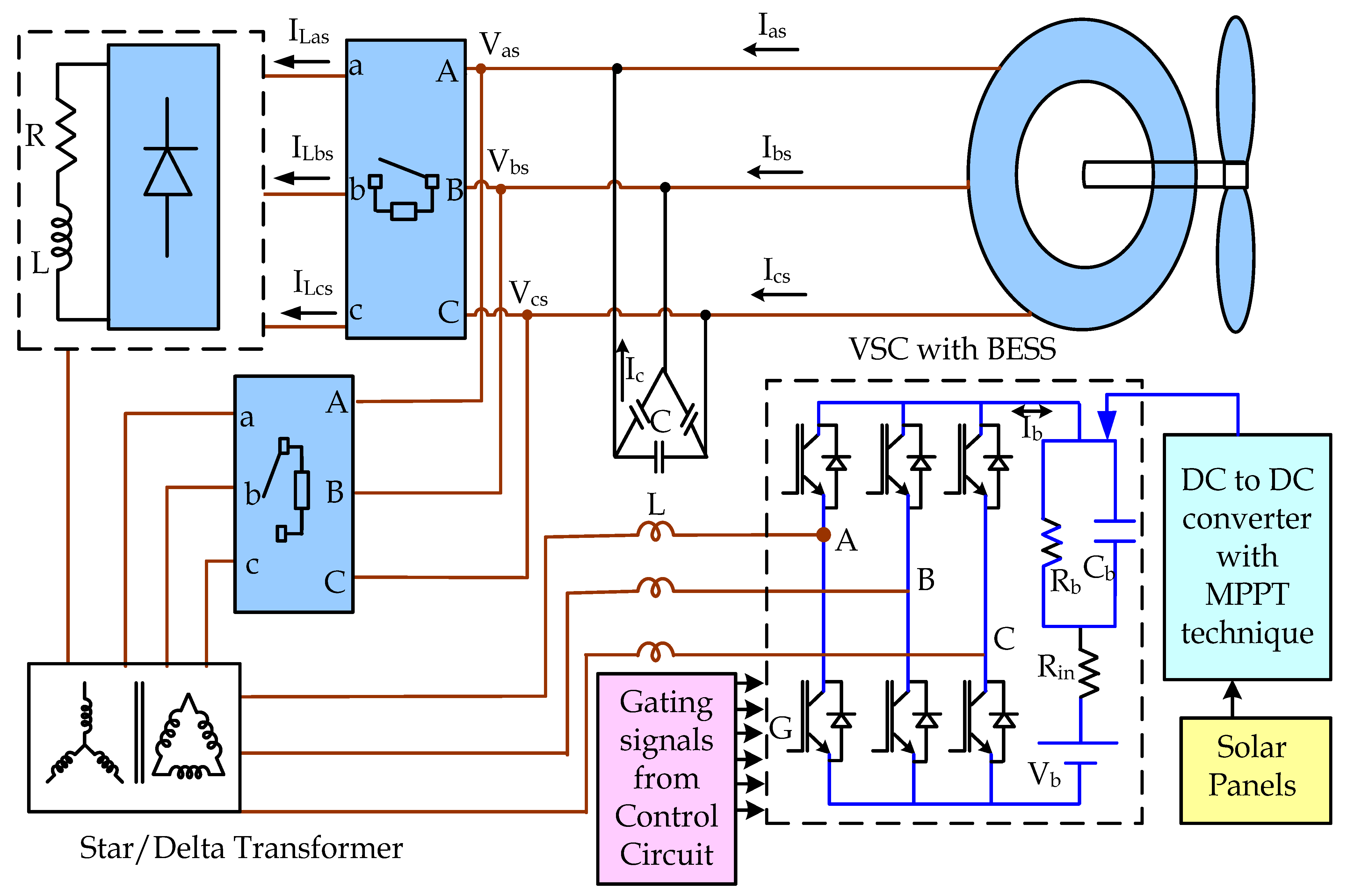
A solar photovoltaic (PV) panel is connected such that the output of the panel charges the battery. The panel consists of 84 cells connected in series. The open-circuit voltage is 64.2 volts, and the short-circuit current of the panel is 7.8 A. Two modules of the PV unit are connected in series and six modules are connected in parallel. A DC-to-DC converter is used to boost the generated voltage. The efficiency of the PV module is usually improved by employing different maximum power tracking techniques (MPPT). The perturb and observe method is used here. The schematic diagram of the hybrid unit under study is shown in Figure 1. The various system parameters are mentioned in Figure 1. Vas, Vbs, and Vcs are the source voltages; Ias, Ibs, and Ics are the source currents in phase a, phase b, and phase c, respectively. ILas, ILbs, and ILcs are the load currents in phase a, phase b, and phase c, respectively. Ic is the current supplied by the excitation capacitor and Ib is the battery current. Vb is the battery voltage and is selected as 400 V. Rin is the internal resistance of the battery and is taken as 0.1 Ω, Cb is the battery capacitance and is 50,000 F; Rb is the resistance of the capacitor and is 10 kΩ, Lf is the filtering inductor and is chosen as 1 mH. Load values in each phase are 30 Ω in series with 0.6 H.
3. Control Algorithm
The enhanced phase locked loop (EPLL) is used as the control algorithm for maintaining the power quality at the wind generating unit and load side. Perturb and observe (P&O) is used as the maximum power point tracking algorithm.
3.1. Enhanced Phase Locked Loop (EPLL)
The enhanced phase locked loop (EPLL) is employed in the controller to effectively manage the reactive power and thus improve the quality of the delivered power. EPLL is a very simple and efficient method for power quality improvement. The drawback of double-frequency ripples in the basic phase-locked loop circuit is eliminated here, by incorporating an inner loop. For a three-phase balanced system, double-frequency ripples are not present, since they cancel each other. However, when the system becomes unbalanced, these ripples will be present. An EPLL is capable of handling these unbalanced conditions in a three-phase system.
The active and reactive phasors of the reference currents are formulated by combining the error signal with the average value of the in-phase and quadrature currents. The frequency error value is used for the calculation of the in-phase quantity. Error in the voltage value at the point of common coupling (PCC), when compared with the reference value of PCC voltage, is used to calculate quadrature components.
3.1.1. Computing In-Phase Reference Currents
The average magnitude of the voltage at the point of common coupling (PCC) is computed from the wind energy converted voltages (, , and ) as
,, and are the unit components in phase with the phase voltages , , and . These are derived as
The unit quadrature components of voltages , , and are derived from in-phase unit voltages , , and as
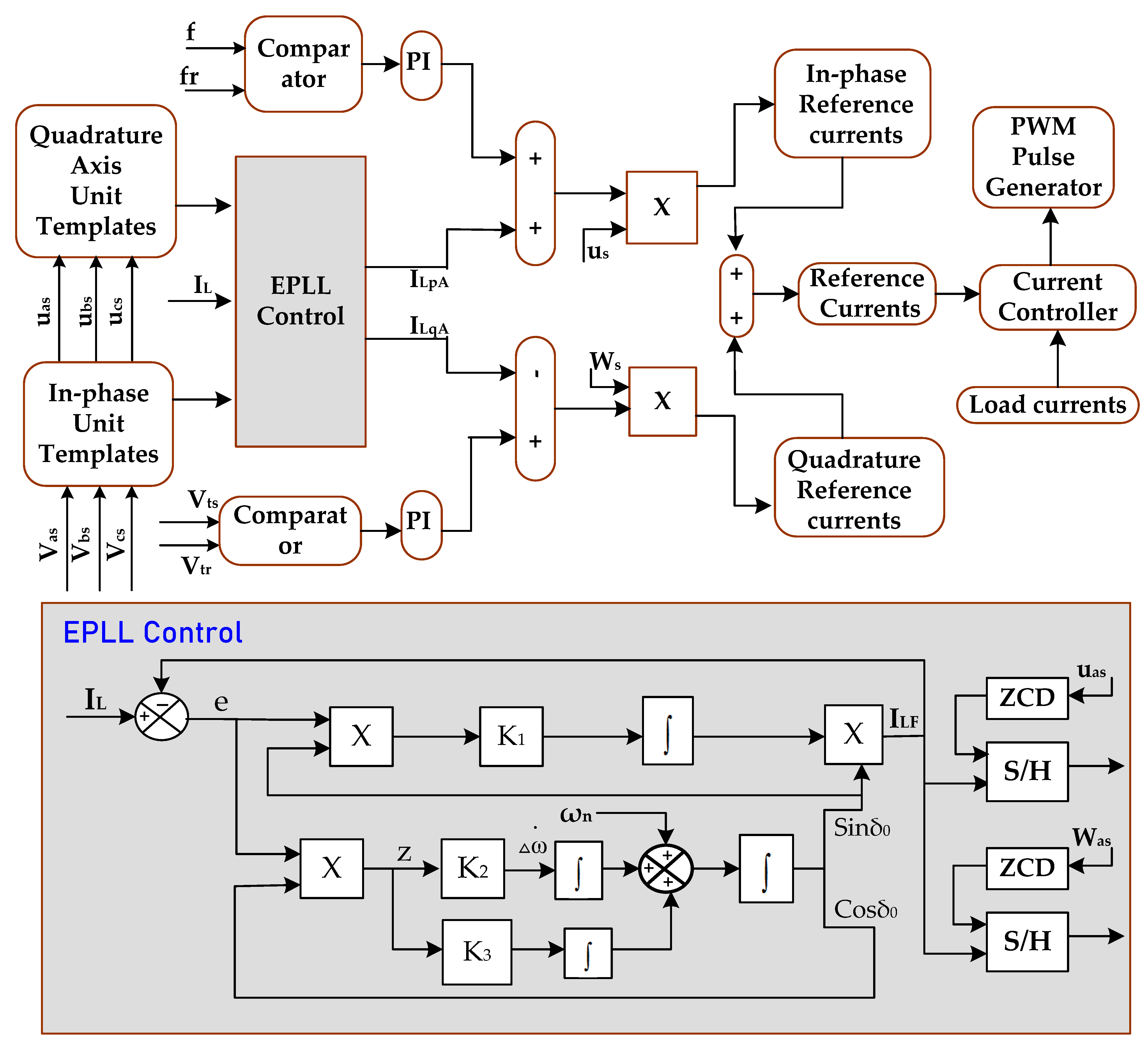
These unit vectors are combined with the load currents to produce the fundamental active and reactive components. These are again processed by combining with frequency error and voltage error appropriately to produce the components of the reference currents. In the enhanced phase-locked loop algorithm, the measured value of load current is compared with the fundamental component of the load current and is connected in a closed-loop. These two signals are continuously compared, and the error signal is produced. This error signal undergoes the process described by Equation (7) to derive the fundamental component of the load current. The control algorithm, along with the enhanced loop description, is given in Figure 2. The fundamental component of current is derived in the inner loop of EPLL. The equations governing this can be given as below:
where is the fundamental value of the current in phase a, and is the error between the actual load current and the fundamental value of the load current. This gives an estimate of the distortion in the signal. is the angle between the fundamental component of current and the actual current. ,, and are the constants that decide the transient and the steady-state behavior of EPLL. The distortion between the fundamental component and the actual load current appears as the error signal. The PI controller works on the error signal to maintain a constant phase angle, which means that the frequency should be the same. The system stability depends upon the value of the gains , , and . The values chosen here are 20, 15, and 1.
The enhanced phase lock loop algorithm uses a zero-crossing detector (ZCD) and a sample and hold (S/H) circuit to produce the fundamental components. The unit vector which is in phase with the applied voltage is made to pass through the ZCD. The zero detector gives the count of the number of times the waveform passes through the zero value. The other input signal to this block is the fundamental component of the load current. By properly combining these two signals, the output of the S/H block gives the phase component of current which goes in phase with the voltage. The average of three-phase components is taken out as the load active power component.
3.1.2. Computing Quadrature-Phase Reference Currents
The quadrature component is also derived in a similar fashion to that of the active components. Here, the quadrature component is made to pass through the ZCD, the output of which is combined with S/H to give a reactive component of current in a particular phase. The average of three-phase components is taken out as the reactive power component of the load current.
The frequency error is produced by comparing the frequency of the measured value of the applied voltage with the reference value. The obtained error signal is modified using the PI gains. The output signal of a sample at the tth instant is given by
The frequency PI controller output at the tth sampling instant is expressed as
where is the active source power at the tth instant. and , respectively, are the proportional and the integral gains of the PI controller. The frequency error is added with the active component of the current and is again multiplied by the unit vectors , , and to generate the active component of the reference current. The voltage error is produced by comparing the terminal voltage with the reference value and amending this error with the controller gains. The voltage error at the tth instant is given by
is the error voltage, is the reference value of terminal voltage, and is the measured voltage. The PI controller output at the tth instant is
This is the reactive power required to maintain a constant terminal voltage at the PCC. The voltage error is added with the reactive component of the current and is again multiplied by the unit vectors , , and to produce the reactive component of the reference current. The total reference current is the sum of active and reactive components.
The measured values of the generated currents , , and are matched with the reference currents , , and . The result is applied to a hysteresis controller to produce the firing pulses for the insulated gate bipolar transistors (IGBT) inside an inverter. These IGBTs are switched on and off according to these gate signals and the compensating current flows to compensate for the distortions in the current.
3.2. Perturb and Observe (P&O)
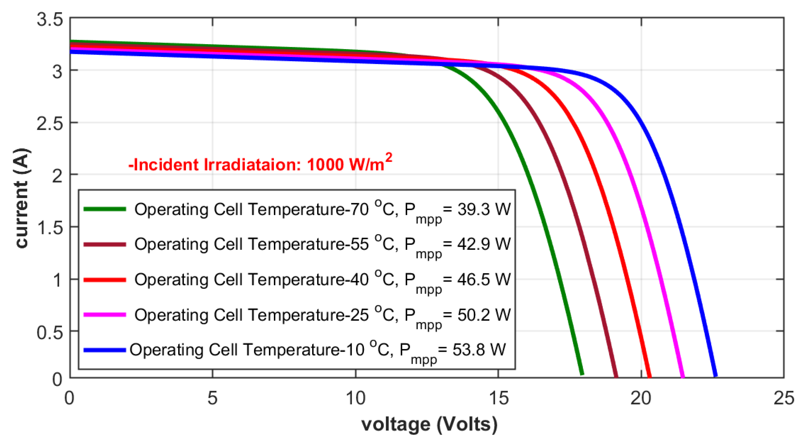
The solar irradiance and the temperature are two important factors that decide the energy output of a solar cell. The I–V characteristics of a solar cell, given in Figure 3, provide information on the current–voltage relationship of a typical solar cell at a particular irradiance and temperature.
As the solar irradiation increases, the produced current increases, but when the temperature increases, the developed voltage decreases. The power generated from a solar panel is at its maximum when the current and voltage are at their maximum values. The current–voltage characteristics help formulate the methods for the solar cell to operate near its maximum power point.
The energy conversion using a solar panel is not very efficient. A normal PV panel is able to convert 11% to 15% of the solar input energy to useable electrical energy. The efficiency of the solar energy conversion is improved by MPPT techniques. These techniques help the PV panel to always operate at its maximum power point by adjusting its duty cycle.
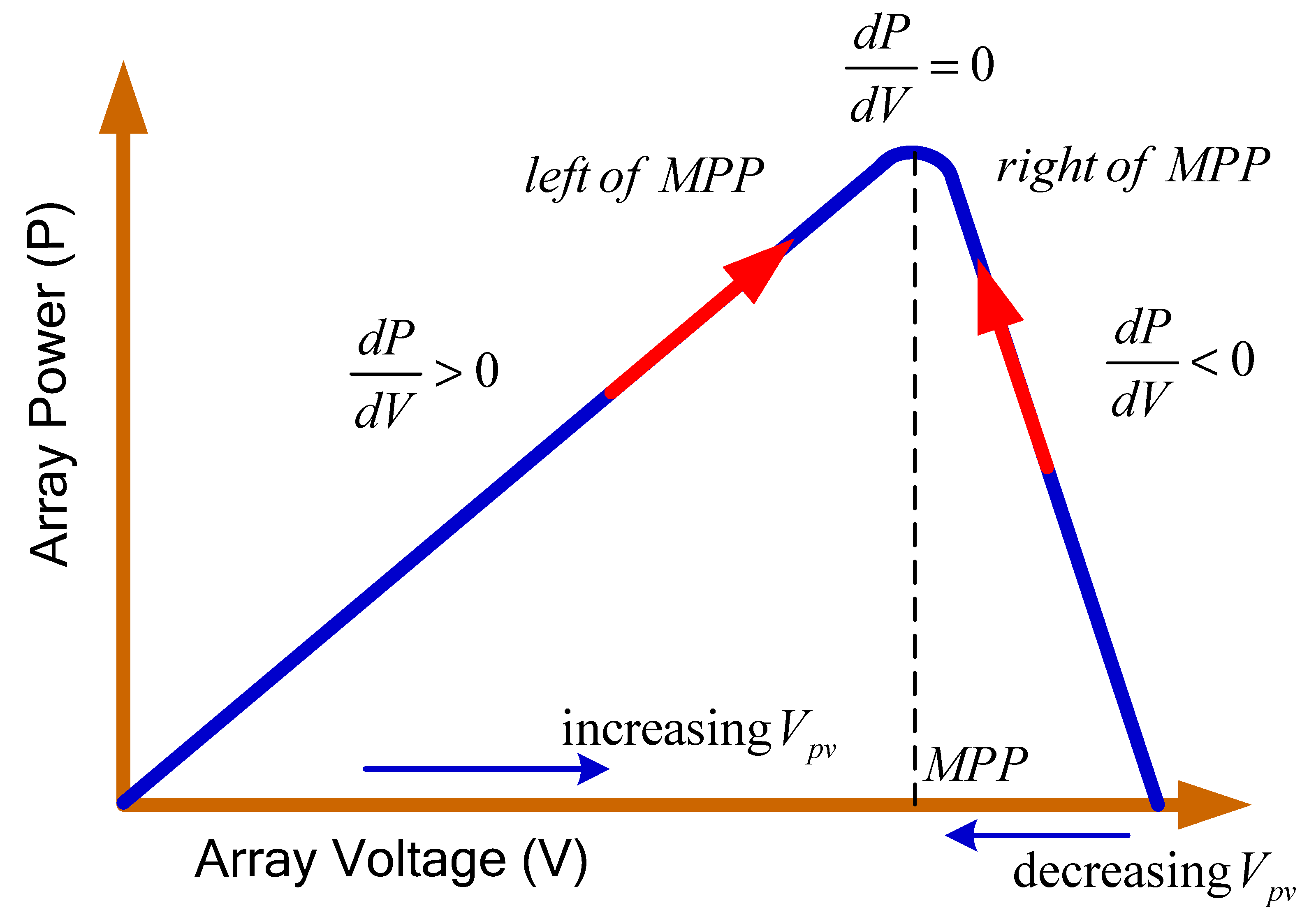
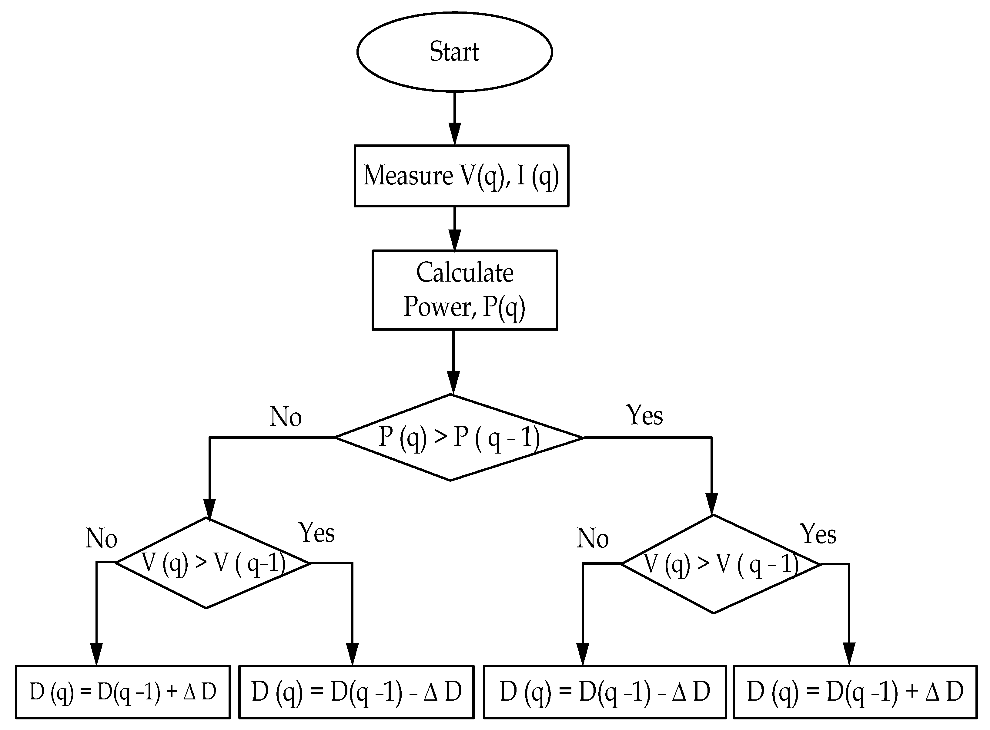
Based on the power–voltage curve shown in Figure 4, the flowchart of the P&O algorithm is explained in Figure 5. In the P&O method, the duty cycle is adjusted in such a way that the power developed in the panel is at its maximum. Power is maximum when the voltage output of the cell and the current flowing are maximum. From the I–V characteristics of the solar cell, any change in voltage from the maximum value causes a reduction in the power extracted. The operating point is adjusted by adjusting the duty cycle of the converter. The relation between the voltage and the power is observed. Suppose an increase in the developed voltage results in an increase in the power, which indicates that the operating point is on the left side of the maximum point in the I–V characteristics, and the duty cycle should be adjusted in such a way that it moves more towards the right side and thus nearer to the maximum point. On the other hand, if an increase in the voltage causes a decrease in the power, that is an indication that the operating point is on the right side of the maximum point and directed towards the left.
4. Optimization of PI Gains
The control circuit provided in the system generates reference signals based on which the triggering pulses are produced. These signals are applied to the voltage source converter to perform the switching operations. Due to these switching operations, the control circuit can effectively compensate for the reactive power, thus improving the power quality. The measured values are compared with the reference values to keep the frequency and terminal voltage constant. The error gets processed through the PI controller. The controller gains are adjusted such that the error value goes to zero.
An optimization problem finds its solution by determining a variable that can minimize or maximize the objective function. After going through several iterations of the fitness calculations and updations in the variables, the algorithm gives an optimal value. The final value of the objective function or fitness function proposes a solution close to the best solution possible. The proposed solution and the rate of convergence help the researcher decide how effective the optimization technique is, to solve a particular problem.
The PI controller gains are usually adjusted by trial and error, which is a lengthy and time-consuming process. Here, various optimization techniques are employed to find out the best values for the PI controller gains. The different techniques used are particle swarm optimization (PSO), selective particle swarm optimization (SPSO), and salp swarm algorithm (SSA). These techniques are applied individually, and results are noted down. The gain values obtained by these techniques are applied in the PI controller. The resultant output waveforms are compared.
All the techniques which are employed here are based on the characteristics of the swarms. Particle swarm optimization (PSO) is a popular technique to find the optimized solution for a problem. A new research area based on swarm intelligence was evolved based on this. PSO mainly refers to the intelligent behavior of a swarm of birds, while searching for food. The location of food is the optimized solution for the bird’s search. In PSO, each particle refers to a potential solution to the problem. By performing continuous updates in the position and the velocity of the particle, the most probable solution is found.
PSO has a very simple concept, and it is easy to implement. It is faster and less complex compared to many other optimization techniques, but it suffers from the disadvantages of having less search precision and falling into local optima while solving complex problems. Many variations of the classical version are proposed in recent times to improve the quality of the solution, speed of convergence and to expand the applicability of the algorithm. Selective particle swarm optimization (SPSO) was suggested in 1997. Here, the search space is selected to give the best possible solution. In SPSO, similar to in a PSO, the velocity and positions of each particle are updated in each iteration. Since the search is confined to the selected search space, the rate of convergence is faster. Salp swarm algorithm (SSA) is a technique inspired by the swarming nature of the salps. Salps, with their barrel− shaped body, resemble jellyfishes. These form chain-like swarms in deep oceans.
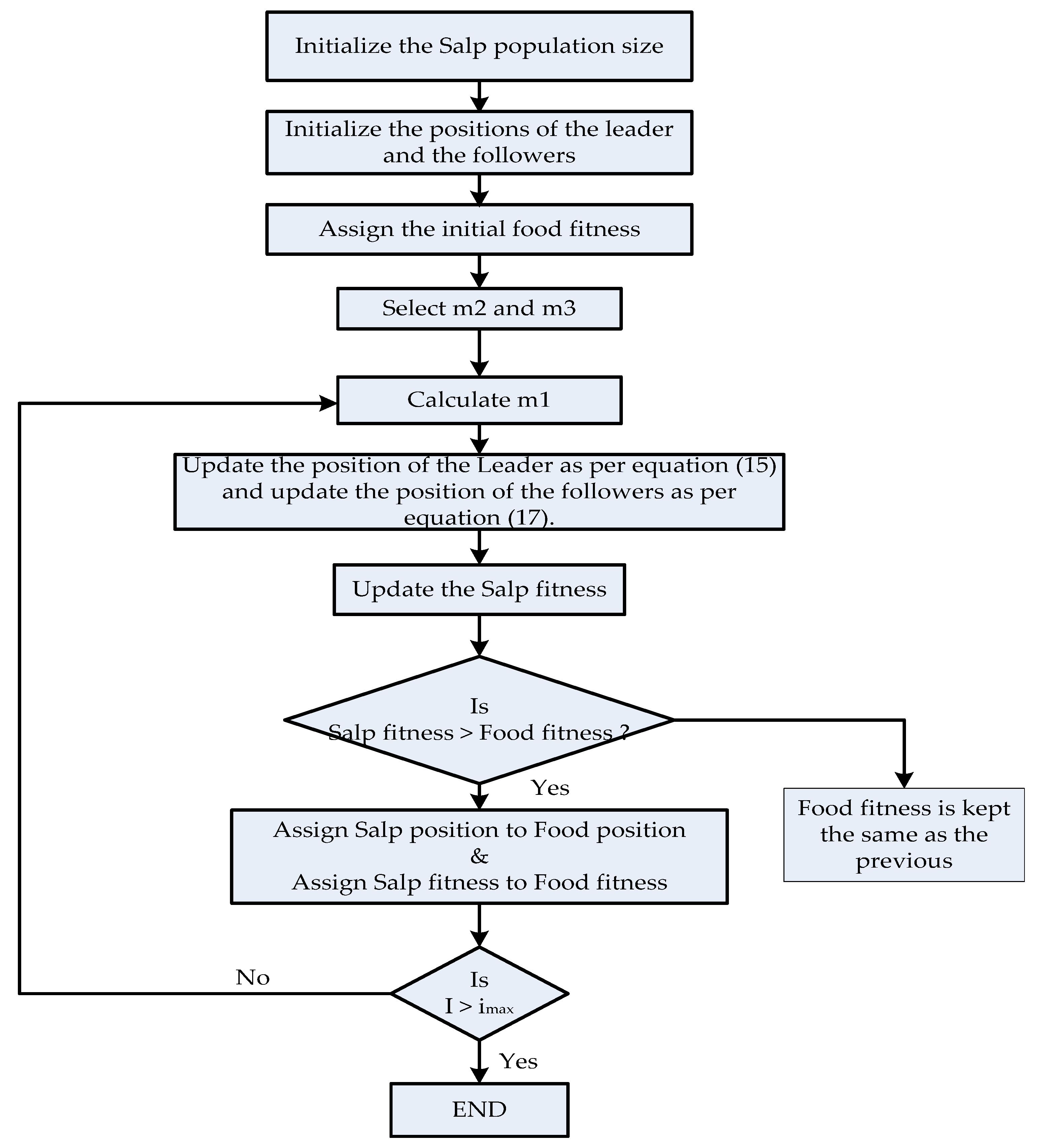
The mathematical model of SSA divides the total population into two parts: the leader and the followers. The first salp in the chain takes the role of the leader. All other salps fall into the category of followers. The swarm is guided by the leader. The followers follow each other and, in that process, ultimately follow the leader. The purpose of the salp chain movement is to chase the source of food called F, which is placed in the search space. To start with, in the algorithm, random positions are assigned to the salps. It computes the fitness of each salp. The positions of the leader and the followers are updated by the respective equations. The algorithm assigns the position of the salp with the best fitness to the position of the food source. The best possible solution or position is taken as the global optimum. This process, except the initialization, is iterative and it continues until the end criterion is met. The search space is limited and is maintained within the boundaries by defining the boundary conditions. An n−dimensional search space with n number of variables is defined. A two−dimensional matrix X stores the positions of salps. In SSA, only the position of the leader is updated with respect to the food source and is given by the following equation:
Here, is the position of the leader in the kth dimension, is the position of the food source in the kth dimension, and are the upper and lower boundaries of the kth dimension. , , and are random numbers. The coefficient is said to balance the exploration and exploitation and plays an important role in the optimization process. The value of is found out by
where is the current iteration and is the maximum iteration. and are random numbers in the range [0,1]. These define if the position of the leader is towards the negative infinity or positive infinity. The follower position is updated by Newton’s second law of motion and is given by
where is the acceleration of the particle and is the initial velocity. In SSA, the food source position is updated according to the leader position. The follower positions are updated with respect to each other, which ensures the gradual movement towards the leader, which in turn helps to avoid the stagnation of local optima. Figure 6 shows the flowchart of SSA algorithm.
The cost function is selected such that the steady-state errors of the PI controllers used in the frequency comparator circuit and the PCC voltage comparator circuit are minimized. The cost function is given by
where and stand for integrated squared error and are the inputs to frequency and AC PI controllers.
and are the weights of and , and are taken as 0.5. The Simulink model workspace data of and are extracted and then given to the algorithms for optimizing PI gains.
The constraints incorporated for the values of Kp and Ki are given as
where Kp1 and Ki1 are the gains of the frequency PI controllers and Kp2 and Ki2 are the gains of the voltage PI controllers.
0 < Kp1 < 5; 0 < Ki1 < 5
0 < Kp2 < 4; 0 < Ki2 < 4
For an easy comparison, the gain values while different optimization techniques are applied to the simulated circuit are tabulated in Table 1.
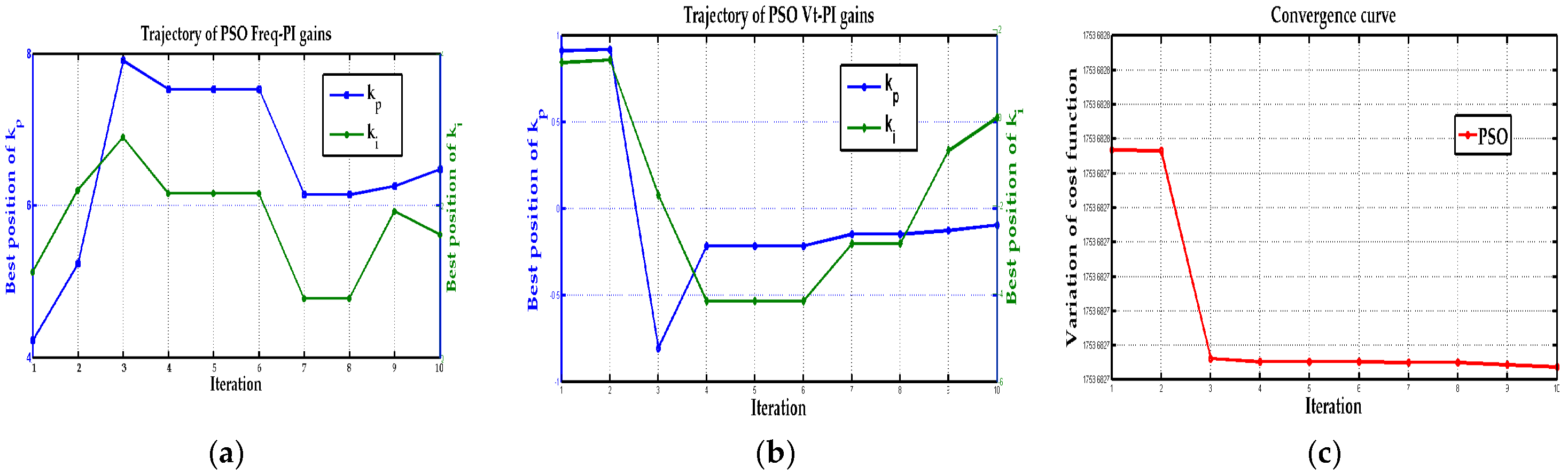
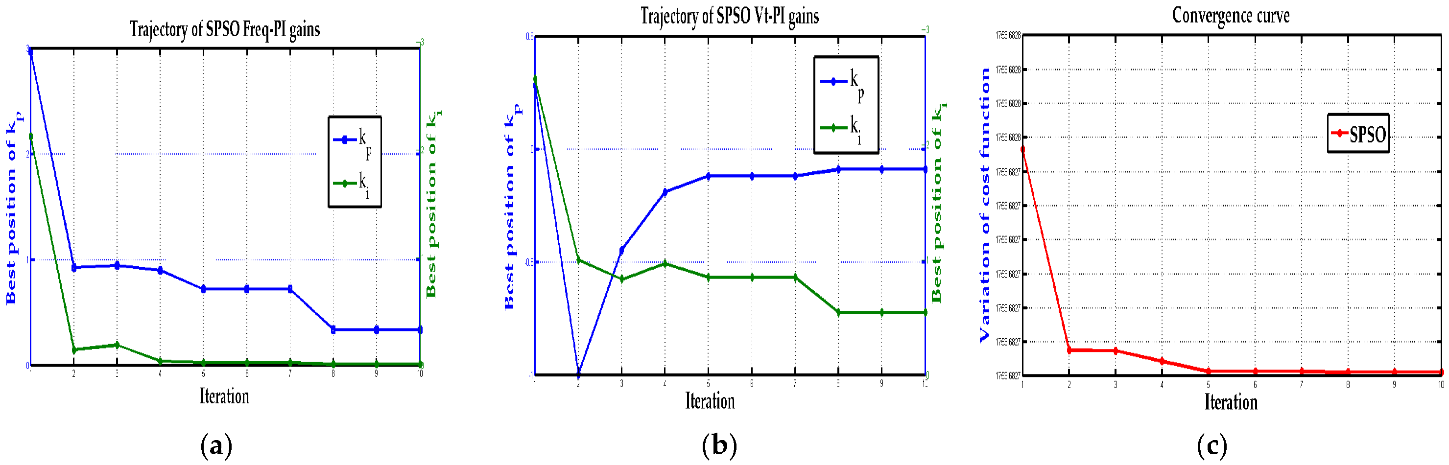
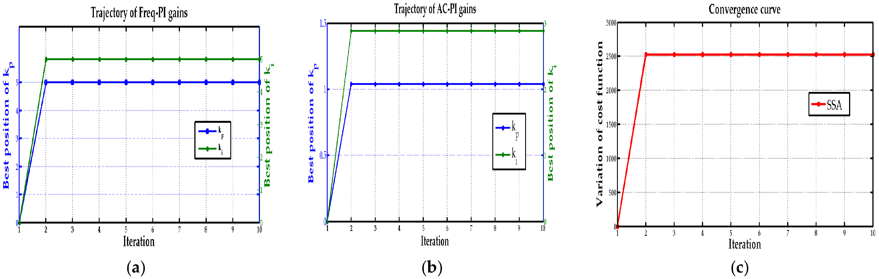
The frequency and Vt gains obtained from the optimization techniques are substituted in the PI controller blocks, and the waveforms of the simulated circuit of the wind generating unit are observed and analyzed. The gain values obtained from SSA gave exemplary waveforms for the output parameters, whereas the values from PSO and SPSO could not produce quality output. The convergence curves refer to the rate at which the algorithm proceeds towards the global optimum. A gradual convergence is preferred to obtain the best optimum solution. The convergence curve of SSA shows that the solution is moderately converged into its best.
5. Simulation Results
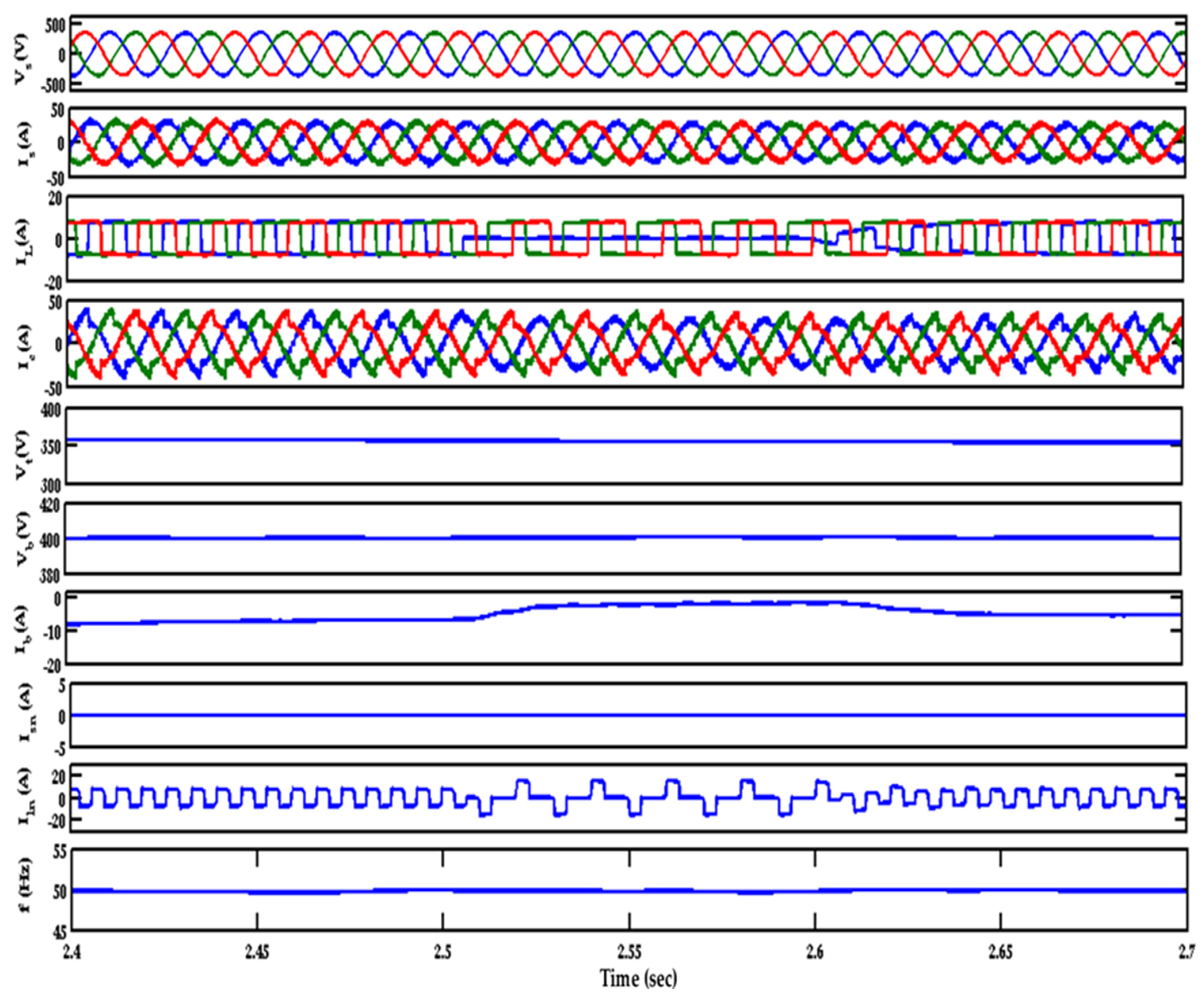
The system under consideration is a wind power generating unit with a 7.5 KW generator. The generator starts developing the power at 0.35 s. The load is linked to the wind generator at 0.35 s. The wind energy conversion system is connected to a star − delta transformer. The delta side of the transformer is connected to the controller. The controller is included in the circuit at 0.5 s. The developed voltage, source current, load current, terminal voltage, frequency, and neutral current are observed during the simulation. The above parameters are monitored for different load conditions, such as linear load and nonlinear load, during the disconnection of a load and the load’s reconnection. Different parameters of the wind energy system under disturbed load conditions are plotted in Figure 10.
The voltage at the generator output terminals, current at the same points, current drawn by the load, the current required to compensate the reactive power requirement, and the terminal voltage and frequency are plotted for the nonlinear load at constant wind speed. The battery current, load neutral current, and source neutral current are also plotted. The load in phase “a” is disconnected at 2.5 s. The controller acts in such a way that the imbalance in the load does not affect the source current. The source current maintains its sinusoidal nature when the load is disconnected and even when it is reconnected. Frequency and terminal voltage are also maintained constant during the load disturbance. When the load is disconnected, the battery current is found positive, which indicates that the battery is charging. This shows the role of the energy storage system in maintaining the system parameters to the reference values. When the load requirement is less than the rated value, the battery charges, accepting the additional power. When the load is restored, the battery current returns to the initial value.
The imbalance in one phase of the load sets up a current in the load neutral. Since the load neutral is connected with the transformer neutral, it becomes circulated between these two, leaving the source neutral current as zero. This helps the source current not to get distorted in case of a disturbance in the load side.
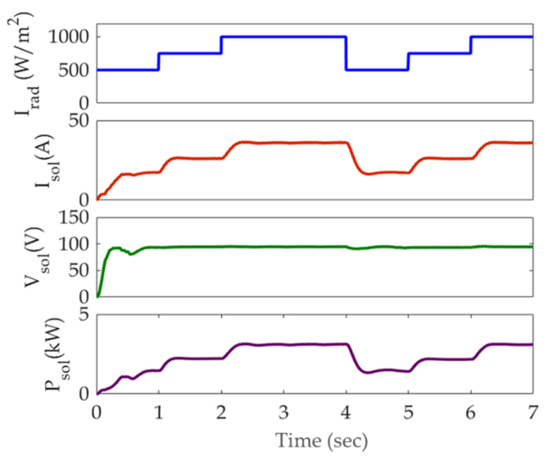
Figure 11 shows the variation in the current, voltage, and power produced in the solar panel, for different values of solar irradiation. The voltage developed in the solar cell is unaffected by the change in the irradiation, but the current and, thus, the power varies proportionally to the irradiation.
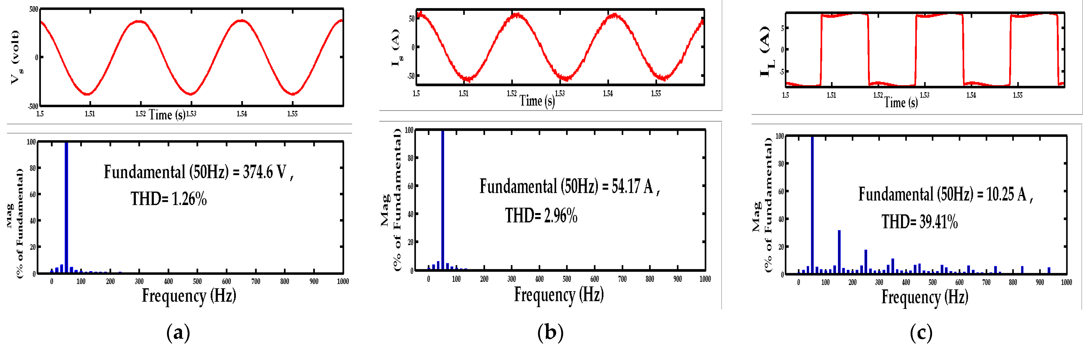
The FFT analysis of the terminal voltage and current waveforms is shown in Figure 12a–c. The displayed total harmonic distortion (THD) values of the generated voltage, generated current, and current at the load side, respectively, when a nonlinear load is connected, are shown. The THD values of the voltage at the generator terminals-generated current and load current was found to be 1.29%, 2.96%, and 39.41%, respectively. As per IEEE 519 standards, all these values are well within their allowable limits. It can be seen that the distortions in the load current are not allowed to pollute the source current, because of the action of the controller.
6. Conclusions
This paper deals with a controller which works very efficiently in maintaining the stability of a system during normal, as well as disturbed, load conditions. The system consists of wind and solar power generating units connected with an energy storage system. The generated power from the wind generator is directly connected to the load. The photovoltaic cell is connected as the alternate source of power, and it charges the battery. The controller works with enhanced phase-locked loop, which controls the power system quality parameters and maintains them at par with the reference values. The EPLL controller algorithm works very efficiently to compensate for the reactive power and thus reduce the harmonics under normal and disturbed load conditions. The double-frequency error, which is the drawback of standard PLL, is eliminated in EPLL by providing an inner loop, thus eliminating the frequency deviations. The battery stores energy when the generated power from the wind unit exceeds the load power. By absorbing and releasing the power according to the load conditions, the battery helps to improve the controller’s efficiency. The perturb and observe method, which is used as the MPPT technique in the solar unit, is a proven technology in improving the efficiency of the solar panel. By properly implementing the control algorithms, the system is made to work very effectively to maintain quality power at the load and the source side. The total harmonic distortion in source voltage and source current are maintained below the limit specified by IEEE 519 standards. The distortions in the load current are not allowed to pollute the source current, because of the action of the controller. The optimization techniques are used to derive the gains of the PI controllers, which helps to fine-tune the system performance. The implementation of the optimization techniques avoids the difficulty of trial and error, thus making the tuning easy. The convergence curve and the trajectory of the gain values show that the tuning with the salp swarm algorithm suits the system better than the other algorithms used, and simulation results validate this conclusion.
In future, the system can be expanded by including a larger number of renewable energy sources.
Author Contributions
Conceptualization, A.K. and R.V.; methodology, R.V. and S.R.S.; software, A.K. and N.R.K.; validation, A.K., R.V., N.R.K. and S.R.S.; formal analysis, A.K.; investigation, R.V.; resources, N.R.K. and S.R.S.; data curation, A.K.; writing—original draft preparation, A.K. and N.R.K.; writing—review and editing, R.V. and S.R.S.; visualization, A.K.; supervision, R.V. and N.R.K.; project administration, R.V. and S.R.S.; funding acquisition, R.V. and S.R.S. All authors have read and agreed to the published version of the manuscript.
Funding
This research work was funded by Woosong University’s Academic Research Funding-2022.
Institutional Review Board Statement
Not applicable.
Informed Consent Statement
Not applicable.
Data Availability Statement
Not applicable.
Conflicts of Interest
The authors declare no conflict of interest.
References
- Giant Leap Forward in Floating Wind: Siemens Gamesa Lands the World’s Largest Project, the First to Power Oil and Gas Offshore Platforms. Available online: https://www.siemensgamesa.com/-/media/siemensgamesa/downloads/en/newsroom/2019/10/pressrelease-siemens-gamesa-hywind-tampen_en.pdf (accessed on 20 January 2022).
- Boro, D.; Donnou, H.E.V.; Kossi, I.; Bado, N.; Kieno, F.P.; Bathiebo, J. Vertical Profile of Wind Speed in the Atmospheric Boundary Layer and Assessment of Wind Resource on the Bobo Dioulasso Site in Burkina Faso. Smart Grid Renew. Energy 2019, 10, 257–278. [Google Scholar] [CrossRef] [Green Version]
- Zamani, H.; Karimi-Ghartemani, M.; Mojiri, M. Analysis of Power System Oscillations from PMU Data Using an EPLL-Based Approach. IEEE Trans. Instrum. Meas. 2017, 67, 307–316. [Google Scholar] [CrossRef]
- Singh, B.; Arya, S.R. Implementation of Single-Phase Enhanced Phase-Locked Loop-Based Control Algorithm for Three-Phase DSTATCOM. IEEE Trans. Power Deliv. 2013, 28, 1516–1524. [Google Scholar] [CrossRef]
- Philip, J.; Singh, B.; Mishra, S. Performance Evaluation of an Isolated System Using PMSG Based DG Set, SPV Array and BESS, In Proceedings of the 2014 IEEE International Conference on Power Electronics, Drives and Energy Systems (PEDES), Mumbai, India, 16–19 December 2014.
- Pathak, G.; Singh, B.; Panigrahi, B.K. Isolated Microgrid Employing PMBLDCG for Wind Power Generation and Synchronous Reluctance Generator for DG System. In Proceedings of the 2014 IEEE 6th India International Conference on Power Electronics (IICPE), Kurukshetra, India, 8–10 December 2014. [Google Scholar]
- Kumar, S.; Verma, A.K. Performance of Grid Interfaced Solar PV System under Variable Solar Intensity. In Proceedings of the 2014 IEEE 6th India International Conference on Power Electronics (IICPE), Kurukshetra, India, 8–10 December 2014. [Google Scholar]
- Verma, A.K.; Singh, B.; Shahani, D. Modified EPLL Based Control to Eliminate DC Component in a Grid Interfaced Solar PV System. In Proceedings of the 2014 6th IEEE Power India International Conference (PIICON), Delhi, India, 5–7 December 2014. [Google Scholar]
- Singh, Y.; Hussain, I.; Singh, B. Power Quality Improvement in Single Phase Grid Tied Solar PV-APF Based System using Improved LTI-EPLL Based Control Algorithm. In Proceedings of the 2017 7th International Conference on Power Systems (ICPS), Pune, India, 21–23 December 2017. [Google Scholar]
- Chandran, V.P.; Murshid, S. Power Quality Improvement for PMSG Based Isolated Small Hydro System Feeding Three-Phase 4-Wire Unbalanced Nonlinear Loads. In Proceedings of the 2019 IEEE Transportation Electrification Conference and Expo (ITEC), Detroit, MI, USA, 8 August 2019. [Google Scholar]
- Liu, C.; Jiang, J.; Jiang, J.; Zhou, Z. Enhanced Grid-Connected Phase-Locked Loop Based on a Moving Average Filter. IEEE Access 2019, 8, 5308–5315. [Google Scholar] [CrossRef]
- Gude, S.; Chu, C. Dynamic Performance Enhancement of Single-Phase and Two-Phase Enhanced Phase-Locked Loops by Using In-Loop Multiple Delayed Signal Cancellation Filters. IEEE Trans. Ind. Appl. 2020, 56, 740–751. [Google Scholar] [CrossRef]
- Gude, S.; Chu, C.-C. Dynamic Performance Improvement of Multiple Delayed Signal Cancelation Filters Based Three-Phase Enhanced-PLL. IEEE Trans. Ind. Appl. 2018, 54, 5293–5305. [Google Scholar] [CrossRef]
- Golestan, S.; Guerrero, J.; Vasquez, J.C. Single-Phase PLLs: A Review of Recent Advances. IEEE Trans. Power Electron. 2017, 32, 9013–9030. [Google Scholar] [CrossRef]
- Golestan, S.; Guerrero, J.; Vasquez, J.C. Three-Phase PLLs: A Review of Recent Advances. IEEE Trans. Power Electron. 2016, 32, 1894–1907. [Google Scholar] [CrossRef] [Green Version]
- Luo, S.; Wu, F. Improved Two-Phase Stationary Frame EPLL to Eliminate the Effect of Input Harmonics, Unbalance, and DC Offsets. IEEE Trans. Ind. Inform. 2017, 13, 2855–2863. [Google Scholar] [CrossRef]
- Xie, M.; Zhu, C.Y.; Shi, B.W.; Yang, Y. Power Based Phase-Locked Loop Under Adverse Conditions with Moving Average Filter for Single-Phase System. J. Electr. Syst. 2017, 13, 332–347. [Google Scholar]
- Golestan, S.; Guerrero, J.; Gharehpetian, G.B. Five Approaches to Deal with Problem of DC Offset in Phase-Locked Loop Algorithms: Design Considerations and Performance Evaluations. IEEE Trans. Power Electron. 2015, 31, 648–661. [Google Scholar] [CrossRef] [Green Version]
- De Carvalho, M.M.; Medeiros, R.L.P.; Bessa, I.V.; Junior, F.A.C.; Lucas, K.E.; Vaca, D.A. Comparison of the PLL Control techniques applied in Photovoltaic System. In Proceedings of the 2019 IEEE 15th Brazilian Power Electronics Conference and 5th IEEE Southern Power Electronics Conference (COBEP/SPEC), Santos, Brazil, 1–4 December 2019. [Google Scholar]
- Liu, B.; Zhuo, F.; Zhu, Y.; Yi, H.; Wang, F. A Three-Phase PLL Algorithm Based on Signal Reforming Under Distorted Grid Conditions. IEEE Trans. Power Electron. 2014, 30, 5272–5283. [Google Scholar] [CrossRef]
- Agrawal, S.; Nagar, Y.K.; Palwalia, D.K. Analysis and implementation of shunt active power filter based on synchronizing enhanced PLL. In Proceedings of the 2017 International Conference on Information, Communication, Instrumentation and Control (ICICIC), Indore, India, 17–19 August 2017. [Google Scholar]
- Ramezani, M.; Golestan, S.; Li, S.; Guerrero, J.M. A Simple Approach to Enhance the Performance of Complex-Coefficient Filter-Based PLL in Grid-Connected Applications. IEEE Trans. Ind. Electron. 2017, 65, 5081–5085. [Google Scholar] [CrossRef]
- Wu, C.; Xiong, X.; Taul, M.G.; Blaabjerg, F. Enhancing Transient Stability of PLL-Synchronized Converters by Introducing Voltage Normalization Control. IEEE J. Emerg. Sel. Top. Circuits Syst. 2020, 11, 69–78. [Google Scholar] [CrossRef]
- Yang, C.; Huang, L.; Xin, H.; Ju, P. Placing Grid-Forming Converters to Enhance Small Signal Stability of PLL-Integrated Power Systems. IEEE Trans. Power Syst. 2020, 36, 3563–3573. [Google Scholar] [CrossRef]
- Golestan, S.; Guerrero, J.M.; Vidal, A.; Yepes, A.G.; Gandoy, J.D.; Freijedo, F.D. Small-Signal Modeling, Stability Analysis and Design Optimization of Single-Phase Delay-Based PLLs. IEEE Trans. Power Electron. 2015, 31, 3517–3527. [Google Scholar] [CrossRef] [Green Version]
- Touti, E.; Zayed, H.; Pusca, R.; Romary, R. Dynamic Stability Enhancement of a Hybrid Renewable Energy System in Stand-Alone Applications. Computation 2021, 9, 14. [Google Scholar] [CrossRef]
- Sahoo, S.; Prakash, S.; Mishra, S. Power Quality Improvement of Grid-Connected DC Microgrids Using Repetitive Learning-Based PLL Under Abnormal Grid Conditions. IEEE Trans. Ind. Appl. 2017, 54, 82–90. [Google Scholar] [CrossRef]
- Sun, G.; Li, Y.; Jin, W.; Bu, L. A Nonlinear Three-Phase Phase-Locked Loop Based on Linear Active Disturbance Rejection Controller. IEEE Access 2017, 5, 21548–21556. [Google Scholar] [CrossRef]
- Escobar, G.; Ibarra, L.; Valdez-Resendiz, J.E.; Mayo-Maldonado, J.C.; Guillen, D. Nonlinear Stability Analysis of the Conventional SRF-PLL and Enhanced SRF-EPLL. IEEE Access 2021, 9, 59446–59455. [Google Scholar] [CrossRef]
- Hadjidemetriou, L.; Kyriakides, E.; Blaabjerg, F. A Robust Synchronization to Enhance the Power Quality of Renewable Energy Systems. IEEE Trans. Ind. Electron. 2015, 62, 4858–4868. [Google Scholar] [CrossRef]
- Zhong, Q.-C.; Boroyevich, D. Structural Resemblance Between Droop Controllers and Phase-Locked Loops. IEEE Access 2016, 4, 5733–5741. [Google Scholar] [CrossRef]
- Sun, D.; Long, H.; Zhou, K.; Wu, F.; Sun, L. An Improved αβ -EPLL Based on Active Disturbance Rejection Control for Complicated Power Grid Conditions. IEEE Access 2019, 7, 139276–139293. [Google Scholar] [CrossRef]
- Kamran, M.; Mudassar, M.; Fazal, M.R.; Asghar, M.U.; Bilal, M.; Asghar, R. Implementation of improved Perturb & Observe MPPT technique with confined search space for standalone photovoltaic system. J. King Saud Univ.–Eng. Sci. 2018, 32, 432–441. [Google Scholar]
- Salman, S.; Ai, X.; Wu, Z. Design of a P-&-O algorithm based MPPT charge controller for a stand-alone 200W PV system. Prot. Control Mod. Power Syst. 2018, 3, 25. [Google Scholar]
- Bodha, V.R.; Srujana, A.; Kuthuri, N.R. Predictive back-to-back SCHVC for renewable wind power system for scrutinizing quality and reliability. Energy Sources Part A Recovery Util. Environ. Eff. 2019, 41, 3058–3075. [Google Scholar] [CrossRef]
- Sattenapalli, S.; Manohar, V.J. Performance analysis of reference current generation methods with pi controller for single-phase grid connected PV inverter system. J. Green Eng. 2019, 9, 658–672. [Google Scholar]
- Tiruye, G.A.; Besha, A.T.; Mekonnen, Y.S.; Benti, N.E.; Gebreslase, G.A.; Tufa, R.A. Opportunities and Challenges of Renewable Energy Production in Ethiopia. Sustainability 2021, 13, 10381. [Google Scholar] [CrossRef]
- Juma, M.I.; Mwinyiwiwa, B.M.M.; Msigwa, C.J.; Mushi, A.T. Design of a Hybrid Energy System with Energy Storage for Standalone DC Microgrid Application. Energies 2021, 14, 5994. [Google Scholar] [CrossRef]
- Aguilar, R.S.; Michaelides, E.E. Microgrid for a Cluster of Grid Independent Buildings Powered by Solar and Wind Energy. Appl. Sci. 2021, 11, 9214. [Google Scholar] [CrossRef]
- Al-Quraan, A.; Al-Qaisi, M. Modelling, Design and Control of a Standalone Hybrid PV-Wind Micro-Grid System. Energies 2021, 14, 4849. [Google Scholar] [CrossRef]
- Farooq, Z.; Rahman, A.; Hussain, S.M.S.; Ustun, T.S. Power Generation Control of Renewable Energy Based Hybrid Deregulated Power System. Energies 2022, 15, 517. [Google Scholar] [CrossRef]
- Tariq, M.; Zaheer, H.; Mahmood, T. Modeling and Analysis of STATCOM for Renewable Energy Farm to Improve Power Quality and Reactive Power Compensation. Eng. Proc. 2021, 12, 44. [Google Scholar] [CrossRef]
- Khan, Z.A.; Imran, M.; Altamimi, A.; Diemuodeke, O.E.; Abdelatif, A.O. Assessment of Wind and Solar Hybrid Energy for Agricultural Applications in Sudan. Energies 2022, 15, 5. [Google Scholar] [CrossRef]
- Tran, Q.T.; Davies, K.; Sepasi, S. Isolation Microgrid Design for Remote Areas with the Integration of Renewable Energy: A Case Study of Con Dao Island in Vietnam. Clean Technol. 2021, 3, 804–820. [Google Scholar] [CrossRef]
- De Doile, G.N.D.; Rotella Junior, P.; Rocha, L.C.S.; Bolis, I.; Janda, K.; Coelho Junior, L.M. Hybrid Wind and Solar Photovoltaic Generation with Energy Storage Systems: A Systematic Literature Review and Contributions to Technical and Economic Regulations. Energies 2021, 14, 6521. [Google Scholar] [CrossRef]
- Montisci, A.; Caredda, M. A Static Hybrid Renewable Energy System for Off-Grid Supply. Sustainability 2021, 13, 9744. [Google Scholar] [CrossRef]
- Eltamaly, A.M.; Alotaibi, M.A.; Alolah, A.I.; Ahmed, M.A. IoT-Based Hybrid Renewable Energy System for Smart Campus. Sustainability 2021, 13, 8555. [Google Scholar] [CrossRef]
- Das, S.R.; Ray, P.K.; Sahoo, A.K.; Ramasubbareddy, S.; Babu, T.S.; Kumar, N.M.; Elavarasan, R.M.; Mihet-Popa, L. A Comprehensive Survey on Different Control Strategies and Applications of Active Power Filters for Power Quality Improvement. Energies 2021, 14, 4589. [Google Scholar] [CrossRef]
- Yoshida, Y.; Farzaneh, H. Optimal Design of a Stand-Alone Residential Hybrid Microgrid System for Enhancing Renewable Energy Deployment in Japan. Energies 2020, 13, 1737. [Google Scholar] [CrossRef] [Green Version]
- Golestan, S.; Matas, J.; Abusorrah, A.M.; Guerrero, J.M. More-stable EPLL. IEEE Trans. Power Electron. 2022, 37, 1003–1011. [Google Scholar] [CrossRef]
- Orosz, T.; Rassõlkin, A.; Kallaste, A.; Arsénio, P.; Pánek, D.; Kaska, J.; Karban, P. Robust Design Optimization and Emerging Technologies for Electrical Machines: Challenges and Open Problems. Appl. Sci. 2020, 10, 6653. [Google Scholar] [CrossRef]
Figure 1.
Layout of the hybrid system under study.

Figure 2.
EPLL control technique.

Figure 3.
Current–voltage characteristics for different temperatures.

Figure 4.
Power–voltage curve in MPPT.

Figure 5.
Perturb and observe algorithm for MPPT.

Figure 6.
Flowchart of SSA.

Figure 7.
(a) Frequency gain; (b) Vt gain; (c) convergence curve for PSO algorithm.

Figure 8.
(a) Frequency gain; (b) Vt gain; (c) convergence curve of the SPSO algorithm.

Figure 9.
(a) Frequency gain; (b) Vt gain; (c) convergence curve for SSA algorithm.

Figure 10.
Performance characteristics of a wind energy unit with a nonlinear load.

Figure 11.
Solar voltage, current, and power at different irradiations.

Figure 12.
THD in (a) source voltage; (b) source current; (c) load current.


Table 1.
Gain values obtained from different optimization techniques.
| Algorithm | Frequency PI Gains | AC PI Gains | Suitability of the Optimization Algorithm | ||
|---|---|---|---|---|---|
| Kp | Ki | Kp | Ki | ||
| PSO | 6.5 | 1.7 | −0.9 | 0 | Not suitable |
| SPSO | 0.3 | 0 | 1.8 | 0.6 | Not suitable |
| SSA | 5 | 5 | 1.1 | 2.8 | Suitable |
Publisher’s Note: MDPI stays neutral with regard to jurisdictional claims in published maps and institutional affiliations. |
© 2022 by the authors. Licensee MDPI, Basel, Switzerland. This article is an open access article distributed under the terms and conditions of the Creative Commons Attribution (CC BY) license (https://creativecommons.org/licenses/by/4.0/).
Share and Cite
MDPI and ACS Style
Kodakkal, A.; Veramalla, R.; Kuthuri, N.R.; Salkuti, S.R. An Optimized Enhanced Phase Locked Loop Controller for a Hybrid System. Technologies 2022, 10, 40. https://0-doi-org.brum.beds.ac.uk/10.3390/technologies10020040
AMA Style
Kodakkal A, Veramalla R, Kuthuri NR, Salkuti SR. An Optimized Enhanced Phase Locked Loop Controller for a Hybrid System. Technologies. 2022; 10(2):40. https://0-doi-org.brum.beds.ac.uk/10.3390/technologies10020040
Chicago/Turabian StyleKodakkal, Amritha, Rajagopal Veramalla, Narasimha Raju Kuthuri, and Surender Reddy Salkuti. 2022. "An Optimized Enhanced Phase Locked Loop Controller for a Hybrid System" Technologies 10, no. 2: 40. https://0-doi-org.brum.beds.ac.uk/10.3390/technologies10020040
Note that from the first issue of 2016, this journal uses article numbers instead of page numbers. See further details here.