
Flow Stress Description Characteristics of Some Constitutive Models at Wide Strain Rates and Temperatures

1
Mechanics of Materials and Design Laboratory, Department of Materials Engineering, Gangneung-Wonju National University, 7 Jugheon-ghil, Gangneung 25457, Gangwon-do, Korea
2
Agency for Defense Development, P.O. Box 35-5, Yuseong, Daejeon 34186, Korea
*
Author to whom correspondence should be addressed.
Technologies 2022, 10(2), 52; https://0-doi-org.brum.beds.ac.uk/10.3390/technologies10020052
Submission received: 6 March 2022
/
Revised: 20 March 2022
/
Accepted: 1 April 2022
/
Published: 11 April 2022
Abstract
:The commonly employed mathematical functions in constitutive models, such as the strain hardening/softening model, strain-rate hardening factor, and temperature-softening factor, are reviewed, and their prediction characteristics are illustrated. The results may assist one (i) to better understand the behavior of the constitutive model that employs a given mathematical function; (ii) to find the reason for deficiencies, if any, of an existing constitutive model; (iii) to avoid employing an inappropriate mathematical function in future constitutive models. This study subsequently illustrates the flow stress description characteristics of twelve constitutive models at wide strain rates (from 10−6 to 106 s−1) and temperatures (from absolute to melting temperatures) using the material parameters presented in the original studies. The phenomenological models considered herein include the Johnson–Cook, Shin–Kim, Lin–Wagoner, Sung–Kim–Wagoner, Khan–Huang–Liang, and Rusinek–Klepaczko models. The physically based models considered are the Zerilli–Armstrong, Voyiadjis–Abed, Testa et al., Steinberg et al., Preston–Tonks–Wallace, and Follansbee–Kocks models. The illustrations of the behavior of the foregoing constitutive models may be informative in (i) selecting an appropriate constitutive model; (ii) understanding and interpreting simulation results obtained using a given constitutive model; (iii) finding a reference material to develop future constitutive models.
1. Introduction
The manufacturing of ductile materials via high-speed machining, such as drilling, milling, friction stir welding, and explosive welding, often leads to strain rates of the deforming material higher than 105 s−1 [1]. A given material can also experience a wide range of temperatures, from cryogenic to melting point, in manufacturing processes such as cryogenic machining [2] and laser ablation [3,4,5,6]. Similar or even more severe loading rates and temperature conditions are involved when ductile materials encounter ballistic or high-speed impacts [7], penetration [8], blasting, and explosion [9]. Consequently, the ranges of strain rates and temperatures considered herein are from 10−6 to 106 s−1 and from absolute to melting temperatures, respectively. To precisely model and simulate the foregoing events for design/understanding purposes, a reliable constitutive model that can describe the flow stress of ductile materials in such a wide range of strain rates and temperatures is indispensable, together with an equation of the state and fracture model, if necessary.
When a ductile material deforms plastically, the associated flow stress generally exhibits strain hardening/softening, strain rate hardening, and temperature softening. Numerous types of constitutive models with various formulations have been proposed via physically based or phenomenological approaches to describe the strain rate and temperature dependence of the flow stress–strain curve. Researchers who investigate the deformation behavior of solids at a wide range of strain rates and temperatures generally aim to select constitutive models that can reasonably describe their materials. In general, however, the experimental data were not available in the original papers of the constitutive models at sufficiently wide strain rates and temperatures compared with the mentioned ranges above; the flow stress description capabilities of the proposed models were verified in limited ranges of strain rates and temperatures.
The motives of this review paper (i.e., the raised problems (issues) herein) are that the above circumstance imposes difficulties on researchers in (i) selecting an appropriate model to describe their materials at a wide range of strain rates and temperatures; (ii) understanding and interpreting simulation results obtained using the selected constitutive model; (iii) finding a reference material to develop future constitutive models for a wide range of strain rates and temperatures.
In general, a list of formulations of numerous constitutive models is prepared before selecting an appropriate model. However, the list itself does not help much in solving the aforementioned difficulties. Consequently, to assist in solving the raised problems above, this review paper aims to provide three contributions as follows.
First, this paper illustrates how the mathematical functions, which were commonly employed in constitutive models, contribute to the flow stress (Section 3). The mathematical functions include stress–strain curve models, strain-rate hardening factors, and temperature-softening factors. The foregoing functions considered herein were selected purely based on the experience of the authors, but the result may include the majority of the functions commonly employed in constitutive models. The illustration result should assist in understanding the flow stress description characteristics of the constitutive model that employs the functions.
Second, this study presents how the available constitutive models themselves describe the phenomena of strain hardening/softening, strain rate hardening, and temperature softening in a wide range of strain rates and temperatures (Section 4 and Section 5). There is no general consensus for selecting only a few of the constitutive models for review purposes among numerous ones in the literature. Eleven constitutive models were selected herein purely based on the experience of the authors. One more constitutive model (see Acknowledgments) was selected in accordance with the comments of an anonymous reviewer. As a result, six phenomenological and six physically based models were considered herein. The phenomenological models included the Johnson–Cook [10], Shin–Kim [11], Lin–Wagoner [12], Sung–Kim–Wagoner [13], Khan–Huang–Liang [14], and Rusinek–Klepaczko [15,16] models. The physically based models were the Zerilli–Armstrong [17,18], Voyiadjis–Abed [19], Testa et al. [20], Steinberg et al. [21,22,23], Preston–Tonks–Wallace [23,24,25], and Follansbee–Kocks [23,26,27,28,29,30,31] models. To illustrate how these selected models behave at wide strain rates and temperatures, this review paper neither carried out new experiments nor newly calibrated the constitutive models. Instead, the calibrated constitutive parameters of the materials considered in the original papers of the models were employed. Then, the model-predicting flow stress was calculated herein from absolute to melting temperatures and strain rates from 10−6 to 106 s−1. As shown later, this simple approach revealed the strong points and drawbacks of the considered models efficiently, assisting in solving the three problems raised above. The elucidated characteristics of the considered models were compared from the viewpoint of model selection.
Finally, to further assist one in solving the problems raised, the origins of some deficiencies of the considered models are disclosed. The origins are revealed in terms of the employed mathematical functions in the considered constitutive models.
2. Constitutive Model
2.1. Definition
A constitutive equation refers to the relationship between stress and strain. The J2-flow theory describes the plastic response of ductile solids in terms of equivalent stress () and equivalent strain () [32,33]:
where and are the components of the deviatoric stress and strain tensors, respectively. The unprimed quantities denote the total stress and total strain components: , , and are normal stresses; , , and are the shear stresses; , , and are normal strains; , , and are shear strains (engineering); , , and are the principal stresses; and , , and are the principal strains.
A constitutive model is the hardening law that characterizes the evolution of the flow stress with increased plastic deformation: the – curve (see Nomenclature). The plastic deformation regime of the stress–strain curve measured under a uniaxial stress state is usually used to calibrate the constitutive model. Under such a stress state, the measured stress–strain curve becomes the – curve.
2.2. Phenomenological Constitutive Model
A reliable constitutive model should reasonably describe the phenomena of strain hardening/softening, strain rate hardening, and temperature softening over a wide range of strains, strain rates, and temperatures. A simple approach to develop a constitutive model may be to model each of the aforementioned phenomena using engineering (phenomenological) functions in the form:
where functions , , and denote the strain hardening/softening model (in Pa), strain-rate hardening factor (non-dimensional), and temperature-softening factor (non-dimensional), respectively. When the individual functions are multiplied to form a constitutive model, as in Equation (3), the constitutive model is called decoupled. The Johnson–Cook (JC) model takes this form (Equation (3)); the detailed form of the JC model is described later. Other conceivable forms of the phenomenological model include the following:
where Fi is the function that couples the influences of any two variables among , , and ; G is the function that couples the influences of all of them. Equation (3) describes the fully decoupled form, Equation (4) the partially coupled forms, and Equation (5) the fully coupled form. The strain hardening/softening model (), strain-rate hardening factor (), and temperature-softening factor () used in the fully decoupled form (Equation (3)) of the phenomenological model are often employed in the partially decoupled forms (Equation (4)). Other forms of phenomenological models that employ summation frameworks together with multiplication frameworks (Equations (3)–(5)) exist, which are shown later.
To calibrate the constitutive models, the flow stress–strain curves need to be measured accurately not only in quasi-static tests at ambient temperatures [34,35,36] but also in a wide range of strain rates and temperatures. Examples of the calibration results can be found in the original papers of the considered models herein.
2.3. Physically Based Constitutive Model
Physically based modeling of the flow stress with plastic deformation is based on the dislocation dynamics, which considers dislocation movement and its accumulation. At strain rates less than approximately 104 s−1 [37,38], thermally activated dislocation motion is opposed by short-range and long-range obstacles [17,18]. The short-range barriers are overcome by thermal activation, whereas the long-range barriers are independent of temperature (athermal). The short-range barriers include forest dislocations in face-centered cubic (FCC) materials, Peierls–Nabarro barriers in body-centered cubic (BCC) materials, and other origins such as point defects, alloy elements, solute atoms, impurities, and deposits. The long-range barriers include grain boundaries, far-field dislocation forests, and other microstructural origins with far-field influence.
Based on this reasoning, flow stress is regarded as the material resistance to dislocation motion and is often considered to be composed of thermal and athermal components. As ductile materials are polycrystalline, the theory of crystal plasticity [39] that relates the deformation of individual crystals with the slip needs to be combined with the polycrystal plasticity model [40]; the individual grain response is linked to the overall behavior of polycrystalline aggregates. At strain rates higher than approximately 104 s−1, the mechanism of dislocation drag, which includes the inertia effect [41], is predominantly considered for dislocation motion.
3. Mathematical Functions in Constitutive Models
The engineering (mathematical) functions introduced for phenomenological models, , , and , are also often employed as a part of the physically based models, like in the six physically based models considered herein. Once a physically based model employs such a function, it may be called a semi-physically based model on a strict base. However, it considers the physical mechanisms described in Section 2.3. as the main skeleton of the model, while a phenomenological model does not consider such mechanisms. In this regard, the former is called a physically based model herein (instead of the semi-physically based model).
The knowledge of the influences of mathematical functions (i.e., , , and ) on flow stress should be informative in analyzing the descriptive characteristics of constitutive models (either phenomenological or physically based). Accordingly, this study first illustrates the variation of , , and with the change in their parameters, which will assist in their proper usage. Subsequently, the analysis results of the mathematical functions will be used to interpret the description characteristics of six phenomenological and six physically based models.
3.1. Stress–Strain Curve Models
3.1.1. Strain Hardening Models
While the phenomenon of strain hardening in the plastic deformation regime results from dislocation movement-based crystal plasticity [42,43], its phenomenology can be described using some forms of engineering functions (). This section reviews several available forms of strain hardening models: the models by Hollomon, Swift, Ludwik, and Voce.
The Hollomon model [44] is:
where k and n are fitting parameters, called the hardening constant and hardening exponent, respectively. Equation (6) is also called the power-law model. The value of k in Equation (6) is the stress when the strain value is unity. The value of n describes how rapidly the stress rises when ε < 1; a smaller n value results in a rapid increase in stress. However, the smaller n value results in a slower increase when the strain value is fairly large (ε >1)
The Swift strain hardening model [45] is:
where k, n, and are the fitting parameters. This model replaces in Equation (6) with ; the stress–strain curve of Hollomon () offsets along the strain axis by a value of −.
The Ludwik strain hardening model [46] is of the form:
where A, B, and n are the fitting parameters. Parameter A shifts the stress–strain curve of the Hollomon model () along the stress axis by an amount of A (yield strength). Parameter B describes the amount of strain hardening after yielding until the strain reaches unity. As in Equations (6) and (7), n controls how rapidly the flow stress increases after yielding.
The Voce strain hardening model [47] is as follows:
where A, B, and C are the fitting parameters. As in the Ludwik model, parameter A is the yield strength. Parameter B is related to the amount of strain hardening when strain hardening is saturated. A larger C value results in a more rapid increase in stress after yielding.
The previously mentioned physical meanings of A, B, and C (i.e., A, B, and n in the Ludwik model) are informative in the calibration process of the strain hardening model. For instance, the meanings can be referred to in setting-up the initial guess values of the parameters when modeling the experimental stress–strain curve using Equations (8) or (9). The meanings are also useful in checking whether the calibrated parameters are physically admissible.
A linear combination of the Ludwik [46] and Voce [47] models can be considered as follows:
where α is the parameter () that controls the proportion of the two models. Equation (10) is a six-parameter model, because A1 = A2 = A. Various types of flow stress–strain curves can be flexibly described, as this model employs more (six) fitting parameters as compared with the foregoing models with two to three parameters.
3.1.2. Strain Hardening/Softening Model
After strain hardening, ductile materials often exhibit strain softening (see Figure 1), which eventually leads to fracture. According to the ductile damage model built in Abaqus [32] and GISSMO in Ls-Dyna [33], damage (D) initiates from the maximum flow stress point (D = 0) and couples with the strain hardening constitutive behavior thereafter, which decreases the flow stress with strain after the maximum-flow-stress point (see Figure 1a). In such coupled damage models, fracture is assumed to occur when the damage value reaches unity (D = 1). Elements with such damage values are eliminated in the explicit finite element simulation, which leads to a load drop in the simulated structure (the description on the damage localization is omitted here to abide by the subject of this study—constitutive behavior).
Damage can also be modeled as uncoupled with the constitutive behavior. In such uncoupled damage models, fracture criteria can be based on many physical quantities such as stress triaxiality, Lode parameter, and mixed strain/stress state. The simplest fracture criterion may be the fracture equivalent strain criterion, which is employed in the “shear failure” fracture model in Abaqus [32], the failure option in the “piecewise linear plasticity” material model in LS-Dyna [33], and versatile material/fracture models in many finite element codes such as Autodyn [9] and Dytran [48]. In the foregoing uncoupled damage model, elements with such a critical value of equivalent strain (fracture equivalent strain) are eliminated in the explicit finite element simulation [9,48].
Uncoupled models generally have the advantages of easy implementation in finite element codes and few parameters to identify compared with coupled damage models. Their disadvantage is that the decrease in load-carrying capacity after the maximum load is rarely described. This disadvantage can be overcome if the strain softening part of the stress–strain curve is modeled as part of the constitutive model. For instance, in [49,50,51], the strain hardening as well as the softening part of the stress–strain curve was regarded as constitutive behavior. Both parts were inputted to simulation code as the constitutive behavior, and fracture was assumed to have occurred when the employed uncoupled fracture criterion (e.g., fracture equivalent strain criterion) was met. Subsequently, the characteristic feature of Ti6Al4V (serrated chip) was successfully simulated by employing the strain hardening/softening constitutive model and an uncoupled fracture model.
The following mathematical functions are proposed herein to model the strain hardening/softening behavior of the stress–strain curve shown in Figure 1b. When
or
When
where is the maximum (critical) flow stress at : or respectively. The above way of modeling enables one to describe the deformation behavior of strain hardening/softening material efficiently (see Figure 1b). If the fracture behavior of the strain hardening/softening material needs to be simulated, an uncoupled fracture model (e.g., fracture equivalent strain model or triaxility- and Lode parameter-dependent model) can be employed conveniently.
3.2. Strain-Rate Hardening Factors
This section reviews several available forms of the strain-rate hardening factors () considered in existing studies. The function is hereafter referred to as the rate factor.
3.2.1. Power-Law Rate Factor
According to Kleemola and Ranta–Eskola [52], J.H. Hollomon (Metals Technology, vol. 13, Tech Publication, No. 2034, 1946) used the power-law form to describe the strain-rate dependence of the flow stress:
where q (in Pa) and p (dimensionless) are the fitting parameters. The exponents, bases, and arguments of a mathematical function are non-dimensional. Thus, the variable in the base in Equation (12) is understood herein as , where (dimension controller) value is set as 1 s−1 herein. Any reported (calibrated) values of q and p have meanings only when the unit and magnitude of are specified. As observed in Hosford and Caddell [53], Equation (12) subsequently leads to the relation:
where is the flow stress at . Analyzing Equation (13) in accordance with Equation (3) (, , , and the rate factor, is:
Equation (14) is called the power-law rate factor, where p is the fitting parameter and is the reference strain rate at which the constitutive model that employs Equation (14) is calibrated. is usually set arbitrarily as an interested/convenient value (e.g., 1 s−1) in the calibration process; is a set parameter. The rate factor value becomes unity at , thereby simplifying the strain-rate-dependent constitutive model under the framework of to the form at .
Equation (14) was employed as the rate factor in constitutive models such as the Lin–Wagoner [12] and Khan–Huang–Liang [14] models. Allen, Rules, and Jones [54,55] also employed Equation (14) in their study but was limited to 1 s−1. The role of in their study was limited to the role of the dimension controller that made the base of the exponential function non-dimensional.
The variation of the power-law rate factor with log (/) is illustrated in Figure 2 for different values of c. Although the change in the power-law function with its independent variable is not new, Figure 2 is presented herein as it will also be used later as the comparison reference for other rate factors such as the Cowper–Symonds and Shin–Kim factors. As can be observed in Figure 2, shifts the rate factor curve along the abscissa, which flexibly describes the log (/) dependence of the flow stress as compared with the case where is fixed to a constant (e.g., unity in Allen, Rules, and Jones [54,55]).
The in Equation (14) can be regarded as the fitting parameter in the calibration process of the constitutive model that employs Equation (14). In such a case, because the symbol is generally reserved for the setting variable, it may be appropriate to express Equation (14) as:
where c (s−1 unit) and p (dimensionless) are the two fitting parameters. The employment of Equation (15) in a constitutive model means that the strain rate (c) at which the rate factor becomes unity is determined in the calibration process using the experimental data, instead of being set arbitrarily by the user (Equation (14)). In this regard, Equation (15) is a modified version of the power-law rate factor (Equation (14)).
3.2.2. Wagoner Rate Factor
Wagoner [12] modified the power-law rate factor as:
where and are the two fitting parameters. herein has the same definition and characteristics as those described in the previous section. A modified version of Equation (16) with two fitting parameters (i.e., and ) was introduced in [13] as:
The factor in the exponent and argument of the logarithmic function in Equations (16) and (17), respectively, are understood herein as , where (dimension controller) is 1 s−1.
The variation in the Wagoner rate factor with log (/) is illustrated in Figure 3. m1 and γ1 in Figure 3a,b, respectively, control the curve slope at . As observed in Figure 3b, this rate factor can result in a negative strain-rate dependence in the regime where depending on . In a separate test (resulting figures not shown), and in Figure 3a,b, respectively, were proportional to the slope of the curves at = .
3.2.3. Cowper–Symonds Rate Factor
Cowper and Symonds introduced their rate factor as [55,56,57,58]:
where C and P are fitting parameters with units of (time)−1 and unity, respectively. This rate factor adds unity to a power-law rate factor form (Equation (15)), which offsets the vs. log (/) curve by unity along the vertical () axis (Figure 4a). In Equation (18), parameter C controls the strain rate at which the rate factor value becomes two instead of unity because of the addition of unity. Parameter P controls the curve shape at a given C value, as in the case of the power-law factor (Figure 2).
The Cowper–Symonds rate factor was implemented indeed in many material models in commercial software (LS-Dyna [33]) and was also considered in many studies [55,56,57,58], despite the drawbacks below. As observed in Figure 4a, it is difficult to make the Cowper–Symonds rate factor value unity at a specific strain rate by controlling the C and P values. In Figure 4a, this rate factor reaches unity only when the strain rate is zero; the reference strain rate that makes this rate factor value unity is 0 s−1. Because infinite time is required to measure a stress–strain curve at 0 s−1, the reference stress–strain curve ( in Equation (3)) is rarely measured at such a strain rate. Therefore, the reference stress–strain curve of the Cowper–Symonds rate factor (at 0 s−1) is unfamiliar to researchers. If the power-law rate factor (Equation (14)), its modified version (Equation (15)), or the Shin–Kim (SK) rate factor (discussed later) is employed in a constitutive model, the reference strain rate can be set at, for instance, 0.01–1.0 s−1, which is close to the quasi-static strain rate that can be routinely achieved in a laboratory. Then, the reliability of the calibrated values of the constitutive parameters of the reference stress–strain curve () can be checked (verified) suitably because the reference stress–strain curves of the foregoing models are not much different from the familiar curves routinely measured in a laboratory. Thus, the power-law rate factor, its modified version, and SK rate factor are desirable for use as compared with the Cowper–Symonds factor.
If the rate factor value can be made unity at an ambient condition (e.g., 0.01–1.0 s−1) like in the foregoing rate factor models, the temperature softening factor () can be conveniently calibrated using additional stress–strain curves measured at different temperatures but at the mentioned condition. In other words, the admissibility of the calibration result can be readily checked at an ambient condition. However, if the Cowper–Symonds rate factor is employed, the calibration result cannot be readily verified because the rate factor value cannot be made unity at an ambient condition (but at 0 s-1). Overall, no benefit is found for adding unity to the power law-type factor (Equation (15)), which results in the Cowper–Symonds model and sets the value as 0 s−1.
In the Cowper–Symonds rate factor, the slope of the rate factor curve in the quasi-static regime (log (/) < 0) and that in the high strain-rate regime (log (/) > 0) cannot be independently controlled. For instance, in Figure 4a, consider the curve for p = 0.5 when log (/) < 0. This curve is positioned at the bottom among the considered ones. If then, the slope of this curve (p = 0.5) should be most rapid when log (/) > 0. Other slow-slope curves (for instance, p = 0.00625) are not allowed in the regime where log (/) > 0. This characteristic is also similarly observed in the power-law (Equation (14) and Figure 2) and modified power-law (Equation (15)) rate factors. However, in the SK rate factor (introduced later), the slope of the rate factor curve when log (/) < 0 and the rate factor value at log (/) > 0 can be varied independently.
3.2.4. Johnson–Cook (JC) Rate Factor
The JC constitutive model [10] employs a rate factor:
where C is a fitting parameter. As mentioned, is a set parameter at which all of the parameters of the overall constitutive model employing Equation (19) are calibrated. The variation of the JC rate factor with log (/) depending on the C values is illustrated in Figure 4b. This rate factor describes a linear increase in the flow stress () with log (/), which is a major limitation in that it cannot describe the stress upturn phenomenon, which will be described later.
3.2.5. Huh–Kang Rate Factor
The Huh–Kang rate factor [59] is:
where c1 and c2 are the two fitting parameters; in the argument of the logarithmic function is understood herein as the quantity divided by the unit strain rate , where is 1 s−1.
The variation of the Huh–Kang rate factor with log (/) depending on c1 and c2 is illustrated in Figure 5. c1 controls the slope of the curves at = , whereas c2 controls the curve slope when . This rate factor can result in a negative strain-rate dependence in a low strain-rate regime at depending on the c2 value. Setting values other than unity in Equation (20) modifies the Huh–Kang rate factor to flexibly describe the rate hardening behavior by shifting the curves along the abscissa (as in Figure 2 for the power-law rate factor).
3.2.6. Shin–Kim (SK) Rate Factor
The SK rate factor [11] is:
where D and E are the fitting parameters, is as previously defined. When the value of E is set to zero, Equation (21) approximates the JC rate factor.
The variation in the value of Equation (21) with log (/) depending on D and E is illustrated in Figure 6. In Figure 6, the D value controls the slope of the rate factor curve when , that is, the slope in the linearly rising regime (usually the quasi-static strain-rate regime). The E value controls the onset point of the stress-upturn phenomenon at a given D value. The slope at and the rate factor value at are controlled independently via D and E values, respectively. As aforementioned, the SK rate factor overcomes the limitations of the power-law rate factor (Equation (15)), Cowper–Symonds rate factor (Equation (18), and JC rate factor (Equation (19)).
The stress upturn phenomenon generally occurs at approximately 103 s−1, meaning the E value is generally less than approximately 10−4 s−1 as observed in Figure 6. When , Equation (21) becomes practically unity, because E is a small number.
3.2.7. Lim–Huh Rate Factor
Huh et al. [60] proposed a strain-dependent rate factor as follows:
where q1, q2, q3, and m are the fitting parameters. and in the bases of exponential function in Equation (22) are understood herein as the quantities, each of which is divided by the unit strain rate: and , respectively, where is 1 s−1. Equation (22) is called the Lim–Huh model in [61].
The variation in the value of Equation (22) with log (/) is illustrated in Figure 7a using parameters for 4340 steel [60]: q1 = 0.013, q2 = 0.012, q3 = 0.420, and m = 0.275 when = 10−3 s−1. As observed in Figure 7a, the degree of rate hardening is dependent on the strain value: the higher the strain, the lower the degree of rate hardening. In Figure 7b, where is increased to 10+3 s−1, as anticipated, the reference value of the strain rate controls the strain rate at which the rate factor value becomes unity, and the rate factor curves mainly shift along the log () axis.
As q1 increases by ten times in Figure 7c (from 0.013 to 0.13), the rate factor curves increase more rapidly at , and the vertical gap between the curves increases. As q2 increases by 40 times to 0.48 (Figure 7d), the rate factor curves increase less rapidly at , diminishing the vertical gap between the curves.
As q3 increases three times to 1.26 (Figure 7e), the stress upturn phenomenon is more significant at a smaller strain. As m increases three times to 0.825 (Figure 7f), all the rate factor curves increase more rapidly at , regardless of the strain values, and the influence of m is more or less similar to that of q1 and is roughly inverse to the influence of q2. As this rate factor model employs four fitting parameters (i.e., q1, q2, q3, and m) and one set parameter (), the strain rate dependence of the flow stress can be flexibly described.
3.3. Temperature-Softening Factors
This section reviews some available forms of temperature-softening factors () in previous studies. The function is also referred to hereafter as the temperature factor (TF). As later observed, the thermal softening phenomenon is often inappropriately described in many constitutive models because they employed inappropriate TFs. Thus, to explicitly elucidate the characteristics of TFs using their names, the TFs considered herein are named based on their characteristic thermal softening behavior rather than the names of authors.
The temperature of the material results from the environment (e.g., in hot forming or hot forging) and the heat generated during material deformation owing to plastic work. The temperature in the constitutive model is the current temperature of the material resulting from both sources.
3.3.1. Absolute Temperature-Based Factor
The homologous temperature () is the non-dimensional temperature of a material, expressed as a function of its melting point. The simplest form of homologous temperature may be , which has been used extensively to describe thermally assisted recrystallization [62]. To describe the thermal softening of metals, Gray et al. [63] employed the foregoing form of homologous temperature ( in their TF:
where m is the fitting parameter.
The variation in the value of Equation (23) with T is illustrated in Figure 8a for a range of m values. The value of this TF is unity at the absolute temperature. By this reason, this factor is named herein as the absolute temperature-based factor. As observed in Figure 8a, the m value controls how rapidly the TF decreases with temperature from the value at 0 K (unity).
3.3.2. Limited-Range Temperature Factor
Johnson and Cook [10] employed the following TF in their constitutive model:
where m is the fitting parameter and is the homologous temperature (). The reference temperature () is the temperature at which the parameters of the constitutive model employing Equation (24) are calibrated. is set arbitrarily as the temperature of interest (e.g., 298 K) in the calibration process; is a set parameter. The value of the TF becomes unity when , thereby simplifying the temperature-dependent constitutive model under the framework of to the form at .
Figure 8b illustrates the change in the value of Equation (24) with T for a range of m values. As observed in Figure 8b, this TF is limited in that its value cannot be calculated at because the base on the right side of Equation (24) becomes negative. Because Equation (24) is defined only when , it is herein named as the limited-range TF. Furthermore, for some m values (e.g., m = 0.3), the curve shape is unrealistic near the reference temperature; the TF decreases overly rapidly at around .
3.3.3. Flexible Temperature Factor
To overcome the limitations of the limited-range TF, Khan, Suh, and Kazmi [14] introduced a TF as:
which employed a different form of the homologous temperature () from that in the JC model ().
Shin and Kim [11] also independently overcame the limit of the limited range TF by introducing a TF:
which employed the JC-type homologous temperature (). Note that Equation (26) is simplified to Equation (25). In Reference [11], the function shapes of Equation (26) were illustrated for a range of m values (Figure 8d) with reference to the limited-range TF (Figure 8b).
The curve shape when T0 = 0 K (Figure 8c) is comparable to that of the absolute temperature-based factor (Figure 8a); however, their curve shapes are notably different. As observed in Figure 8d (T0 > 0 K), the TF value of Equation (26), that is, (25), can be calculated at temperatures even below T0, unlike the limited-range factor (Figure 8b). This is because the base for the exponent m in Equation (25), that is, (26), is positive even at T < .
The value of Equation (25), that is, (26), can be made unity at an arbitrary temperature of interest, and thermal softening behavior is very flexibly described. Accordingly, this factor is referred to as the flexible TF herein. All the TFs illustrated in Figure 8 coerce the TF value to zero at the melting point, which is physically natural.
3.3.4. Pseudo-Linear Temperature Factor
Varshni [64] described the temperature dependence of the shear modulus as , where and are the shear moduli at T and 0 K, respectively. A TF () with an exponential function was introduced as:
where α and T1 are fitting parameters.
The variation of Equation (27) with T depending on T1 is illustrated in Figure 9a. Equation (27) describes a roughly linear decrease in flow stress with temperature, which is why this model is called the pseudo-linear TF herein. In Figure 9a, T1 controls the slope of the thermal softening curve. The increase in shifts the curves in Figure 9a downward (not shown). For most T1 values, this TF is not zero at the melting point, which is unrealistic. This TF and the other three TFs illustrated in Figure 9 do not coerce the zero-flow stress at the melting point, unlike the TFs illustrated in Figure 8. However, the Follansbee–Kocks (FK) constitutive model [26,27,28,29,30,31] employed Equation (27). The consequence of employing the pseudo-linear TF is presented later in the FK model section.
3.3.5. Linear Temperature Factor
Hutchinson [65] considered a linear TF:
where is the fitting parameter, and is the reference temperature. The variation of Equation (28) with T depending on the value is illustrated in Figure 9b. Based on Equation (28), the value of this factor is unity at . However, as in the pseudo-linear factor (Figure 9a), this TF becomes zero at Tm only for a specific value of , which limits the role of as a calibration parameter. However, this factor was employed in the models of Steinberg et al. [21,22] and Preston–Tonks–Wallace [24,25]. The consequences of employing this TF are presented later in the respective model sections.
3.3.6. Power-Law Temperature Factor I
According to [13], Zuzin et al. (Zuzin, W.I.; Broman, M.Y.; Melnikov, A.F. Flow Resistance of Steel at Hot Forming. 1964, Metallurgy) introduced a power-law TF as follows:
where is the fitting parameter, and T0 is the reference temperature.
The change in this TF (Equation (29)) with T depending on is illustrated in Figure 9c. This TF describes the ratio of the flow stress at varying temperatures with reference to that at the reference temperature (). It describes a relatively rapid decay of flow stress with the temperature at T < , whereas the flow stress decreases relatively little with the temperature at T > . This TF was employed in the Lin–Wagoner (LW) model [10]. The consequence of employing this factor is presented later in the LW model section.
3.3.7. Power-Law Temperature Factor II
Lubahn and Schnectady [66] considered a different power-law form TF with only one fitting parameter:
where a is the fitting parameter, and Tm is the material constant (melting point). The variation of Equation (30) with T depending on a is illustrated in Figure 9d. Similar to the other TFs in Figure 9, this factor is not zero at Tm for most of a (the fitting parameter). It becomes zero at an excessively low temperature when the a value is tiny, for example, a = 10−5.
4. Phenomenological Constitutive Models
4.1. Johnson–Cook (JC) Model
To describe not only the strain dependence but also the strain rate and temperature dependencies of the flow stress, Johnson and Cook [10] modeled the flow stress as:
where A, B, n, C, and m are the five fitting parameters. When = and (reference state), only the Ludwik strain hardening model (Equation (8)) remains in Equation (31); the parameters A, B, and n then describe the flow stress–strain curve in the reference state. This model probably has been applied most extensively to simulate high strain-rate events.
The JC model parameters for oxygen-free high thermal conductivity (OFHC) copper, available in [10], are listed in Table 1. Using these parameters, the JC model-predicting flow stresses were calculated herein for a wide range of strain rates and temperatures, and the results are presented in Figure 10. The predicted stress–strain curves at 300 K for different strain rates and the curves at = 1 s−1 for different temperatures are presented in Figure 10a,b, respectively. As assumed in this model, the stress–strain curves at strain rates and temperatures different from the reference state ( and ) are determined by multiplying the reference curve by the constants (i.e., rate and temperature factors, respectively).
Therefore, there is no fundamental shape change in the stress–strain curve with the change in strain rate or temperature. The shape of the stress–strain curves in Figure 10a,b resulting from the decoupled framework of Equation (3) will serve as a comparison reference for the stress–strain curves predicted using constitutive models under the coupled frameworks (Equations (4) and (5)), which are introduced later in the LW [12], SKW [13], and ZA-FCC [17,18] model sections.
The changes in flow stress values at = 0.5 are illustrated with log (/) and temperature in Figure 10c,d, respectively. In Figure 10c, the flow stress increases linearly with log (/) because of the employed rate factor (Equation (19) and Figure 4b). As mentioned, in Figure 10d, the temperature softening is described at T > T0. This model should not fail to describe the flow stress over a wide range of strain rates and temperatures for no reason (except for a temperature range below ).
4.2. Shin–Kim (SK) Model
The flow stress of ductile materials generally increases slowly with log () at a low strain rate (the Arrhenius type increase), whereas beyond a certain range of the strain rate (103–104 s−1), the flow stress rapidly turns upward [67,68,69]. This phenomenon, called stress upturn, results from a viscous drag on dislocations at high dislocation velocities. To describe the stress upturn phenomenon and to overcome the limitations of the limited range TF (Equation (24); Figure 8b), Shin and Kim [11] modeled the flow stress as follows:
where A, B, C, D, E, and m are the six fitting parameters. Only the Voce model (Equation (9)) remains at the reference state ( = and ); parameters A, B, and C describe the stress–strain curve in the reference state.
The SK model parameters for OFHC copper, available in [70], are listed in Table 2. Using these parameters, the SK model-predicting flow stresses were calculated herein for a wide range of strain rates and temperatures, and the results are presented in Figure 11. As this model also belongs to the decoupled framework (Equation (3)), the curve shapes in Figure 11a,b are determined by multiplying the constants with the reference curve.
Figure 11c presents the change in flow stress at = 0.5, with log (/) for different temperatures, which illustrates how this model characteristically describes the stress upturn phenomenon using one more rate parameter (E) than the JC rate parameter (C). The necessity of employing one more parameter can be judged in comparison with the JC model (Equation (31) and Figure 10c).
Figure 11d shows the flow stress softening with temperature. The flow stress is described flexibly even at T < Tref because of the employed temperature factor of Equation (25), i.e., (26) shown in Figure 8d. In Figure 11c,d, no reason can be found for why this model should fail to describe the flow stress in wide ranges of strain rates and temperatures.
The reference stress–strain curve does not shift upward or downward solely by the rate factor (Figure 11c), but it shifts as a result of the co-action with the temperature factor (Figure 11d). The flow stress upturn at a high strain rate (Figure 11c) instantly shifts the reference stress–strain curve upward (Figure 11a), resulting in notable increase in plastic work. Subsequently, temperature increases significantly, which lowers the flow stress back to some extent due to the thermal softening. In the case of a shaped charge jet simulation [9], the increased plastic work due to the stress upturn resulted in an increased volume of melt, which is interpreted to occur after significant thermal softening.
4.3. Lin–Wagoner (LW) Model
To describe the change in the shape of the flow stress–strain curve with temperature (coupling of strain hardening with temperature), Lin and Wagoner (LW) [12] described the flow stress based on the framework of :
where , A, C, D, , and m are the six fitting parameters.
The LW model parameters for SS310 steel, available in [12], are listed in Table 3. Using these parameters, the LW model-predicting flow stresses were calculated herein for a wide range of strain rates and temperatures, and the results are presented in Figure 12. As the influence of strain rate is decoupled in this model, in Figure 12a, no fundamental change in the shape of the stress–strain curve is noted with strain rate; the curves at strain rates other than the reference rate are obtained by simply multiplying constants with the reference curve.
As observed in Figure 12b, the curve shape changes with temperature. To describe such coupling, this model employs one more fitting parameter (, A, C, D, and m) than the decoupled model with the Voce hardening law (A, B, C, and m in Equation (32)). In separate trial, when the 300 K curve was multiplied by approximately 0.5, a curve similar to the 1200 K curve were obtained. If multiplied by approximately two, a curve shape different from the 100 K curve was obtained. Therefore, the LW model describes the thermal coupling of the stress–strain curve at cryogenic temperatures (e.g., 100 K), while the predicted curve shapes at ambient and high temperatures seem to be obtained roughly similarly to the case of a decoupled model (Figure 11b) that employs the same Voce function. The price of employing one more parameter reveals its value at T 300 K.
According to the power-law rate factor (Figure 2), a small β value (0.0098 in Table 3) results in a roughly linear increase in the flow stress with log (/), as shown in Figure 12c. The curve shape in Figure 12c will vary if β changes from 0.0098, as shown in Figure 2.
As observed in Figure 12d, this model describes the flow stress softening with temperature from an overly high stress value at 0 K. Because the temperature dependence of the flow stress is not solely described using power-law temperature factor I, (T/T0)m (Figure 9c), but it also employs the Voce-type function, understanding the variations of the σ vs. T/Tm curve with m necessitates some effort. In separate tests (resulting figures not presented herein), the m of this model needed to be negative to describe the decreasing nature of the flow stress with temperature. An m of −0.2 shifted the current curves in Figure 12d (with m = −0.574) upward, whereas an m of −0.9 shifted the current curves downward; the curve shape was always convex down with such changes in m. In the case of SS310, this model predicts a notable flow stress value at the melting point (T/Tm = 1), which is unrealistic.
4.4. Sung–Kim–Wagoner (SKW) Model
To describe the coupling of strain hardening with temperature, Sung, Kim, and Wagoner (SKW) [13] employed the form,
as in the case of the LW model [12]. The function is given by Equation (17). The functions and were selected from the study of Sung et al [13]:
where H, n, α1, α2, V, A, B, and β, and the parameters in Equation (17) (γ1 and γ2) are ten fitting parameters. Equations (17) and (34)–(37) are the SKW model.
The SKW model parameters for DP590 steel, available in [13], are listed in Table 4. Using these parameters, the SKW model-predicting flow stresses were calculated herein for a wide range of strain rates and temperatures, and the results are presented in Figure 13. According to Equation (34), the strain rate dependence of the stress–strain curve is described by multiplying the reference curve (the curve at ) by a constant. Therefore, as illustrated in Figure 13a, there is no fundamental change in the curve shape with the change in strain rate such as in the case of the decoupled models (i.e., JC and SK).
Because the temperature dependence of the stress–strain curve in this model is not solely described using the linear temperature factor (Equations (36) and (37)), but it also employs the Voce-type function (Equation (35)), investigating the variation of the curve shape with temperature is of interest. In Figure 13b, there is indeed a change in the shape of the stress–strain curve with temperature. At 1200 K, even the strain-softening phenomenon is described. In the temperature range from cryogenic temperature (100 K) to approximately 600 K (Figure 13b), the stress–strain curves can be predicted more or less similarly (although not perfectly) using a decoupled model that employs the same Voce function, i.e., by multiplying a reference curve (e.g., the curve at 300 K) by constants. The price of employing ten fitting parameters repays at temperatures higher than approximately 600 K, provided that the shape of the predicted curve in the high-temperature regime is verified.
The log (/) dependence of the flow stress value (at = 0.5) is illustrated in Figure 13c. The influence of the Wagoner strain rate law (Figure 3) employed in Equation (34) appears. The variation in the curve shape depending on the values of and can be inferred from Figure 3.
In Equation (35), the Voce and Ludwik hardening laws are multiplied by two linear temperature factors (Equations (36) and (37)) differently. Thus, the investigation of the appearance of σ vs. T/Tm curves is of interest. Figure 13d shows the σ vs. T/Tm curves (at ε = 0.5) for different temperatures. The collaboration of the functions , , and results in a convex-down and roughly quadratic/linear decrease in the flow stress with temperature. The strain rate dependence of the σ vs. T/Tm curve in Figure 13d is much higher than that of the LW model (Figure 12d). Further study is necessary to elucidate which one (either Figure 13d or 12d) is more realistic. In Figure 13d, the magnitude of the flow stress at the melting point (T/Tm = 1) is still apparent except at an overly slow strain rate. The flow stress at the melting point notably increases with strain rate, which is unrealistic.
4.5. Khan–Huang–Liang (KHL) Model
The degree of strain hardening after yielding generally increases with strain rate in most ductile materials (Figure 10a, Figure 11a, Figure 12a, and Figure 13a). However, the degree of strain hardening of Ti–6Al–4V decreases with the strain rate [14]. Motivated by this observation, Khan, Huang, and Liang (KHL) [14] described the coupling of the influences of strain and strain rate based on the framework of :
where A, B, , , c, and are six fitting parameters, and is the upper-bound strain rate, which was set arbitrarily as 106 s−1 in the original study.
The KHL model parameters for Ti–6Al–4V, available in [14], are listed in Table 5. Using these parameters, the KHL model-predicting flow stresses were calculated herein for a wide range of strain rates and temperatures, and the results are presented in Figure 14. In Figure 14a, this model characteristically describes a diminished degree of strain hardening as the strain rate increases. To describe the coupling of the influences of strain and strain rate on the flow stress, this model employs one more fitting parameter (A, B, n1, n2, and m) than the decoupled model employing the Ludwik hardening law (i.e., A, B, n, and m in Equation (31)). The necessity of employing one more parameter to describe the coupling of strain and strain rate (Equation (38) and Figure 14a) for a given material can be judged by comparing the stress–strain curves at different strain rates in Figure 10a (the JC model that employs the same Ludwik hardening model). In Figure 14a, the degree of strain hardening decreases from approximately 103 s-1, which eventually leads to the disappearance of the strain hardening phenomenon at 106 s-1; the upper-bound strain rate is 106 s-1 (see Table 5). When the strain rate is near the value of the upper bound (e.g., = 105 s−1), the magnitude of the flow stress can be lower than a lower strain rate counterpart (e.g., the curves at 1 and 103 s-1), especially when the strain is high.
As the influence of temperature is decoupled in this model (Equation (38)), the curves at temperatures other than the reference temperature are obtained by multiplying the reference curve with the constants, as in the case of the JC and SK models. Consequently, in Figure 14b, no fundamental difference in the shapes of the stress–strain curves is observed for different temperatures.
Because this model describes the strain rate dependence of the flow stress using not only the power-law rate factor (Equation (14)) but also the Ludwik-type function (Equation (38)), investigating the variation of the flow stress with log (/) is of interest. Figure 14c illustrates the σ vs. log (/) curves (at ε = 0.5) for different temperatures. Interestingly, the values of the flow stress (at = 0.5) reaches a maximum at approximately 103 s−1 and decreases thereafter, which is believed to be unrealistic.
To avoid the appearance of the maximum flow stress, the value was separately set to a higher value, e.g., 108 s−1 (resulting figures not presented herein). As a result, unlike the curves in Figure 11a, similar shapes of the stress–strain curve were observed despite the change in strain rate. The coupling of strain hardening with strain rate was broken if an excessively high value was set.
4.6. Rusinek–Klepaczko (RK) Model
Rusinek, Zaera, and Klepaczko (RK) [15,16] considered the full coupling of the influences of strain, strain rate, and temperature in the framework of :
where and are the strain rates of the lower- and upper-bounds, respectively;, , , , , , , , and are nine fitting parameters.
The RK model parameters for mild steel ES, available in [16], are listed in Table 6. Using these parameters, the RK model-predicting flow stresses were calculated herein for a wide range of strain rates and temperatures, and the results are presented in Figure 15. The dependence of the stress–strain curves at T = 300 K (Figure 15a) and the T dependence of the stress–strain curves at = 1 s−1 (Figure 15b) indicate that there is no apparent change in the shape of the curve with or T, as in the case of a decoupled model, e.g., JC and SK (Equations (31) and (32)).
As observed in Figure 15a, the description capability of the flow stress at high strain rates (e.g., = 106 s−1) is limited. This is because the function cannot be calculated at such a high strain rate. In Figure 15b, the flow stress description capability is also limited at high temperatures (T 900 K), which is because the function cannot be calculated at such high temperatures.
The log (/) dependence of the flow stress ( = 1 s−1; = 0.5) is shown in Figure 15c. The T/Tm dependence of the flow stress (at = 0.5) is shown in Figure 15d. These figures indicate the calculable limits in and the temperature, respectively, which results from the mentioned characteristics of the and functions, respectively.
5. Physically Based Constitutive Models
5.1. Zerilli–Armstrong (ZA) Model
Zerilli and Armstrong (ZA) [17,18] considered the mechanism of dislocation motion depending on the crystalline structure. In FCC materials, dislocations traverse the barriers of forest dislocations, and the thermal activation area decreases with plastic strain because of the increase in dislocation density. In BCC materials, dislocations overcome Peierls–Nabarro barriers, and the thermal activation area is independent of strain. Consequently, the yield stress of FCC materials is considered to be mainly governed by strain hardening, whereas it is primarily governed by strain rate hardening and temperature softening in BCC materials. Consequently, ZA proposed different constitutive relations for FCC and BCC materials. The ZA model also claimed to describe the behavior of HCP materials because of the intermediate characteristics between BCC and FCC materials.
To develop the crystalline structure-dependent constitutive model, ZA employed the Ludwik hardening model () to which a dislocation-mechanics-based term was added to couple the influences of strain, strain rate, and temperature:
where n (dimensionless), C0, C1, C2, C3, C4, and C5 are the seven fitting parameters. in the argument of the logarithmic function in Equation (40) is the quantity that should be divided by the unit strain rate: , where is 1 s−1. In Equation (40), the added term after the Ludwik hardening model describes the coupling phenomenon, , which stems from physics-based dislocation mechanics.
The actual number of fitting parameters in the ZA model are generally fewer than seven because C1 = C5 = 0 for FCC materials (four fitting parameters; the n value is arbitrary); Equation (40) is then in the framework of . For BCC materials, C2 = 0 (six fitting parameters); Equation (40) is then in the framework of .
5.1.1. ZA-FCC Model
The parameters of the ZA-FCC model () for copper, available in [17], are listed in Table 7. Using these parameters, the ZA-FCC model-predicting flow stresses were calculated herein for a wide range of strain rates and temperatures, and the results are presented in Figure 16. In Figure 16a,b, the yield strengths are independent of either the strain rate or temperature because of the employed framework for FCC materials: .
Figure 16a,b illustrate how the curve shape changes with and T, respectively. In Equation (40), an - and T-independent yield strength () is assumed, where the - and T-dependent flow stress is added. Therefore, the curve shape changes with and T under the constraint of a constant yield strength (); strain hardening is coupled with and T mainly because of the constancy. The of annealed copper may be constant within limited ranges of and T. However, unlike the treatment in ZA-FCC model, as-received copper and other FCC materials [37,71,72] show different values with and T.
In Figure 16c, (i) the increase in stress with log (/) is pseudo linear at the cryogenic temperature, whereas the flow stress gradually increases nonlinearly at a higher temperature in a high regime (e.g., when log (/) 2); (ii) the flow stress decreases little with temperature from approximately 900 K. These characteristics are also observed in the ZA-BCC model that is introduced in the next section.
As shown in Figure 16d, the ZA-FCC model also characteristically describes the σ vs. T/Tm curves to be convex down. When the range of is less than approximately 1 s−1, the magnitude of the flow stress is non-negligible at Tm. If the value is 103 s−1, the magnitude of the flow stress at Tm is quite notable and increases further with , which is unrealistic.
5.1.2. ZA-BCC Model
The parameters of the ZA-BCC model () for tantalum, available in [18], are listed in Table 8. Using these parameters, the ZA-BCC model-predicting flow stresses were calculated herein for a wide range of strain rates and temperatures, and the results are presented in Figure 17. In Figure 17a,b, the yield strength is now dependent on both strain rate and temperature because of the employed framework for BCC materials: . Because of this framework, the stress–strain curves in Figure 17a,b shift upward or downward depending on the function value of , which are added to . Note that the curve shapes are identical despite the change in strain rate (Figure 17a) or temperature (Figure 17b) due to the framework for BCC materials (C2 = 0); the strain hardening (the stress–strain curve) is independent of and T in the ZA-BCC model.
As shown in Figure 17c, the ZA-BCC model also predicts a higher strain rate dependence of the flow stress as the temperature increases like the ZA-FCC model does. The two temperature-dependent features mentioned in the ZA-FCC model (Figure 16c) are also observed in Figure 17c. Such characteristics are uniquely observed in the ZA-FCC and ZA-BCC models among the considered models herein.
In Figure 17d, the ZA-BCC model characteristically describes the σ vs. T/Tm curves to be convex down as in the case of copper (ZA-FCC; Figure 16d). It is also noted that when < 103 s−1, the magnitude of the flow stress decreases rapidly at temperatures less than approximately 0.4 Tm; the flow stress decreases overly rapidly at relatively low temperatures. Furthermore, the magnitude of the flow stress is quite notable even at Tm at all the investigated strain rates, which is unrealistic.
5.2. Voyiadjis–Abed (VA) Model
Voyiadjis and Abed [19] noted that the ZA model could not be applied to deformation at high temperatures because of (i) the approximation in the formulation process and (ii) negligence of the influence of strain rate on the thermal activation area. By considering the evolution of dislocation density during plastic deformation in analyzing the thermal activation of dislocations in FCC and BCC materials, VA developed a constitutive model with the framework of as in the ZA-BCC model [17,18]; the Ludwik strain hardening law was employed to which a dislocation mechanics-based term is added to describe the coupling of strain hardening with and T:
where , B, n, , , , q, and p are the eight fitting parameters. in the argument of the logarithmic function in Equation (41) should be the quantity that is divided by the unit strain rate , where is 1 s−1.
The VA model parameters of tantalum, available in [19], are listed in Table 9. Using these parameters, the VA model-predicting flow stresses were calculated herein for a wide range of strain rates and temperatures, and the results are presented in Figure 18. Because of the employed framework (), the stress–strain curves in Figure 18a,b simply shift upward or downward depending on the function value of , which is simply added to . According to Equation (41), the shape of the stress–strain curve is independent of and T.
In Figure 18b, the stress–strain curve does not necessarily shift downward as the temperature increases. The origin of this phenomenon is explained below. The curves of σ vs. show minima at high temperatures (Figure 18c) and the minima of σ vs. T/Tm curves shifts toward higher temperatures with the strain rate in Figure 18d, which is unrealistic.
5.3. Testa et al. (TBRI) Model
As a physically based model for a BCC material that can describe the yield strength at a wide range of strain rates (10−4–107 s−1) and temperatures (0–Tm), Testa, Borona, Ruggiero, and Iannitti (TBRI) [20] described the flow stress as the sum of athermal stress (), thermally activated stress (), and viscous-drag stress ():
where is the pseudo-reference strain rate (the reason for this naming is explained below), and the fitting parameters, , A, T1, T2, and m in Equation (43) describe the thermally activated stress () at . The reference thermal stress () is the thermally activated stress () at and 0 K. in Equation (44) describes the viscous-drag stress () at .
According to Equation (45), is defined for each temperature; the temperature dependence of is plotted in Figure 19 for a range of m values. increases with temperature toward the saturation value of at the melting point. The saturation reference strain rate at Tm () is a set variable ( = 106 s−1 for S508 steel [20]).
According to Equation (45), is a variable that depends on and m; it is not independently set by the user in the calibration of the TBRI model, unlike the reference temperature in other constitutive models (for instance, the JC, SK, and KHL models). Therefore, is referred to herein as the pseudo-reference temperature; “pseudo” means it seems like the reference strain rate in other models if Equation (45) is hidden. As observed in Figure 19, a higher m results in a higher temperature dependence, yielding a lower at a given temperature (T < Tm).
In the framework of the TBRI model, if , the viscous-drag stress () subtracts the flow stress because of the multiplication of a negative () factor to . Accordingly, Equation (42) may need to be modified to include the term only when .
The parameters of the TBRI model for A508 steel are listed in Table 8 [20]. As mentioned in [20], in Equation (42) can be modeled using the Hall–Petch equation. Taking as a fitting parameter, eight fitting parameters exist together with one set parameter ( and one material constant (Tm).
Unlike other considered models herein, the stress–strain curves cannot be predicted solely using the TBRI model, because there is no strain term in the TBRI model. That is, the mathematical form of the reference thermal stress (; thermally activated stress at and 0 K) is open. Accordingly, the Voce model is employed herein () to predict the strain rate- and temperature-dependent stress–strain curves using the TBRI model. In such a case, a, b, and c are added to the fitting parameters; ten fitting parameters exist in the TBRI model to predict stress–strain curves at different strain rates and temperatures.
For the case of A508 steel (m = 9.83 10), was approximately 0 s−1 at 0 K (Figure 19). Thus, the thermally activated stress at 0 s−1 and 0 K () was 407.0 MPa for A508 steel (Table 10). This thermally activated stress value of 407.0 MPa at 0 K and quasi-static loading rate seems to be fairly low, considering that the predicted value of the yield strength was 727.9 MPa at 0 K in [73] based on the values in many studies. Nevertheless, in Table 8 (407.0 MPa) was employed herein as the yield strength of A508 steel at 0 K: (in MPa unit). b and c, which describe the work-hardening behavior after yielding, were determined herein to be 363.77 MPa and 7.226, respectively, by referring to the work hardening part of the stress–strain curve of A508 steel at −15 °C available in [73]. The determination of b and c in this manner further assumes that the work-hardening behavior after yielding is independent of temperature.
Thus far, stress–strain curves at room temperature (300 K) were constructed for a range of strain rates for comparison with other constitutive models (for instance, Figure 17a). However, the thermally activated stress () of A508 steel at room temperature (300 K) cannot be calculated using the parameters listed in Table 10 because the factor, in Equation (43) can be calculated only when m is an integer when tested from unity to 15; this factor cannot be calculated when m is not an integer (e.g., m = 9.83 in Table 10). To construct the stress–strain curves, a range of m values were assumed herein arbitrarily (9.83 1, 2, 5, and 10) such that the values of factor are 0.719, 1.115, 0.965, and 1.000, respectively.
The m value in Table 10 was first modified to unity, and was modeled to be (in MPa). Then, the TBRI model-predicting flow stresses were calculated herein for a wide range of strain rates and temperatures, and the results are presented in Figure 20. According to Equations (42) and (43), the shape of the stress–strain (σ – ε) curve is determined by the multiplication of the reference curve of by rate factor constant and temperature factor constant; the influences of and T are fully decoupled. Accordingly, Figure 20a,b show that there is no change in curve shape with either the strain rate (Figure 20a) or temperature (Figure 20b).
Figure 21 illustrates the variation of the flow stress (at = 0.5) with the strain rate for a range of temperatures. When m = 1 (Figure 21a), the stress upturn phenomenon was described. However, if m increased to two (Figure 21b), the locus of the stress at 900 K was higher than that at 600 K. A similar phenomenon was also observed when m = 10 (Figure 21d), which is physically unrealistic. The order of the curves seemed to be normal if m = 1 and 5. This observation means that the order of the curves, such as the ones in Figure 20a, will be intermixed if m is 2 or 10. The origin for this observation is shown later using the σ vs. T/Tm curves for varying m values.
As mentioned, the stress upturn phenomenon generally onsets at approximately 103–104 s−1 [67,68,69]. As observed in Figure 21, the stress upturn phenomenon at room temperature (300 K) is predicted to onset at approximately 104 regardless of the m value. According to Figure 19, the values of at 300 K (T/Tm = 0.185) are 1.85 × 10⁵, 3.43 × 10⁴, 217.29, and 0.05 s−1 for m = 1, 2, 5, and 10, respectively. Thus, the onset values of the stress upturn phenomenon are predicted to occur at approximately 1.85 × 10⁹, 3.43 × 10⁸, 2.17106, and 500 s−1 for m = 1, 2, 5, and 10, respectively, which means that unless the m value has a specific value, the predicted onset value at room temperature is unrealistic.
Figure 22 illustrates the variation of the flow stress (at = 0.5) with T/Tm for a range of strain rates. When m = 1 (Figure 22a), the loci of the curves continue to decrease up to the melting point. However, the flow stress does not reach zero at Tm and increases with strain rate.
When m = 5 (Figure 22c), the loci of the curves are more or less similar to the ones shown in Reference [20], whereas the 0 K flow stress is excessively high especially at high strain rates, and the flow stress becomes zero as early as at approximately 0.7 Tm. The behavior of the flow stress with temperature is unrealistic when m = 2 and 10 (Figure 22b,d, respectively).
5.4. Steinberg et al. (SCGL) Model
To describe the dependence of shear modulus and yield strength on strain rates, temperature, and pressure-dependent melting, Steinberg, Cochran, Guinan, and Lund (SCGL) [21,22] described the full coupling of strain hardening with strain rate, temperature, and pressure:
where P is the pressure, is the athermal component of the flow stress, is a function describing strain hardening, is the thermally activated component of the flow stress, and are the shear modulus and density, respectively, and and are the respective values at the reference state (T = 300 K, P = 0, and = 0). The strain hardening function, , is given by:
where , n, and are fitting parameters. The thermal component of the flow stress (), which is the only physical quantity that depends on , is calculated numerically using the following equation [74]:
where parameters is the energy required to form a kink, k is the Boltzmann constant, is the Peierls stress, and C1 and C2 are dislocation-related material constants. This model is composed of five parameters to be fitted from the experiment on flow stress (, , β, , and n) and requires eight material constants (, Uk, C1, C2, , , , and ) that can be obtained from existing studies or separate experiments.
The SCGL model parameters of copper, available in [22], are listed in Table 11. Using these parameters, the SCGL model-predicting flow stresses were calculated herein for a wide range of strain rates and temperatures, and the results are presented in Figure 23. A value of zero was assumed. In Figure 23a, the magnitude of the stress–strain curves does not vary significantly despite the notable change in the strain rate. According to Equation (46), only accounts for the strain-rate dependence of the flow stress, whereas the magnitude of is limited by the value (Equation (49)): 20 MPa (Table 11), which is the maximum shift in the stress–strain curves along the vertical axis owing to the change in strain rate.
As will be shown later, when was higher than approximately 103.2 s-1, Equation (49) could not be satisfied although the value varied from zero to (20 MPa). At such a strain rate, the maximum value of 20 MPa was assumed herein for the value. In this way, the stress–strain curve at = 106 s-1 was determined using Equation (46), and the result is shown in Figure 23a.
Figure 23b plots the strain independent nature of , which is governed by Equation (49). It also indicates that the strain rate dependent variation of is at best 20 MPa. Figure 23c illustrates the temperature dependence of the stress–strain curves at = 1 s−1. A notable temperature dependence is observed, which results from the temperature dependence of both (i) the shear modulus (Equation (46)) and (ii) (Equation (49)). Because the amount of change in the temperature-dependent value is limited to 20 MPa (Figure 23d), the notable dependence of flow stress on temperature (Figure 23c) mainly results from the temperature dependence of the shear modulus.
Figure 23e presents the log (/) dependence of the flow stress ( = 1 s−1, = 0.5) for different temperatures. In Figure 23e, the value of the flow stress is weakly dependent on log (/) at all investigated temperatures. As earlier mentioned, only accounts for the strain-rate dependence of the flow stress. Accordingly, (at = 0.5) is plotted as a function of log (/) in Figure 23f. As also mentioned, the value could not be determined when was higher than approximately 103.2 s-1; the value at such a strain rate was assumed as 20 MPa in Figure 23f. In Figure 23e, the vs. log (/) plot with a maximum value of 20 MPa leaves only the marks in the plot of vs. log (/).
Figure 23g shows a notable temperature dependence of the flow stress (at = 0.5), which mainly results from the temperature dependence of the shear modulus (linear temperature factor in Figure 9b) rather than the temperature-dependent (Figure 23h), which varies within the limit of only 20 MPa. As a result of the characteristics of the employed linear temperature factor (Equation (28) with T0 = 300 K; Figure 9b), the magnitude of the flow stress is notable even at the melting point (T/Tm = 1), where the value of the flow stress should be zero (Figure 10d, Figure 11d and Figure 14d).
5.5. Preston–Tonks–Wallace (PTW) Model
To simulate explosive loading and high-velocity impact, Preston, Tonks, and Wallace (PTW) [24,25] modeled the dependence of the plastic strain rate on the applied stress at low strain rates using the Arrhenius form. This form has singular activation energy at zero stress; the deformation rate vanishes at zero stress. Strain hardening was modeled using the Voce law. They merged the flow properties of metals in the thermal activation regime with those in the shock wave limit, where nonlinear dislocation drag effects are predominant. The PTW model was proposed in the form :
where is the normalized flow stress, which is defined as = ; is the shear stress; is the shear modulus; and are the normalized work-hardening saturation stress and normalized yield stress, respectively; the variables p, θ, and s0 are non-dimensional material constants. and are given by:
where the material constants and are the values assumed by at a high temperature and zero temperature, respectively. and are interpreted similarly. Here, k and are dimensionless material constants. The homologous temperature is defined as . The material constant represents the time required for a transverse wave to cross an atom. Therefore, the term in Equations (50) and (51) represents the dimensionless strain-rate variable. is defined as:
where is the density, and M is the mass of an atom. The shear modulus is described by employing the linear temperature factor [65]: , where is the shear modulus at 0 K (P = 0 and = 0) and T1 in Equation (27) is zero.
The parameters, , , , , , , , , , and were fitted from the experiment on flow stress (e.g., (split) Hopkinson bar experiment [75,76,77,78,79,80,81,82,83]) at different strain rates and temperatures. The material constants, , , and are typically obtained from existing studies. The first terms in the braces of Equations (50) and (51) describe the phenomenon of thermally activated dislocation movement in the low strain-rate regime, and the second terms therein delineate dislocation drag through phonons in the high strain-rate regime. The strain hardening behavior is associated with the second term.
The PTW model parameters of tantalum, available in [24], are listed in Table 12. Using these parameters, the PTW model-predicting flow stresses were calculated herein for a wide range of strain rates and temperatures, and the results are presented in Figure 24. The strain rate dependence of the stress–strain curves at T = 300 K is shown in Figure 24a. While the curves in Figure 24a can be obtained at least up to 106 s−1, the flow stress values are predicted to be practically zero regardless of the strain at such a low strain rate (e.g., = 10−6 s−1), which is unrealistic. The coupling of strain hardening with strain rate (change in curve shape with strain rate) is not apparent at approximately > 10−3 s−1.
The temperature dependence of the stress–strain curve at = 1 s−1 is shown in Figure 24b. While the curves can be obtained at least up to 1200 K, no apparent difference exists among curves at above approximately 600 K, which is unrealistic. The coupling of strain hardening with temperature (change in curve shape with temperature) is not apparent.
Figure 24c presents the log (/) dependence of the flow stress ( = 1 s−1, = 0.5) for different temperatures. An approximately linear increase in the flow stress with log (/) is predicted at 100 K. However, as the temperature increases, there are log (/) ranges where vs. log (/) curves at different temperatures are superposed; the higher the temperature, the wider the superposition range in log (/), which is unrealistic.
Figure 24d shows the temperature dependence of the flow stress (at = 0.5) for different strain rates. When the strain rate is less than approximately 1 s−1, the flow stress decreases rapidly at temperatures below approximately 0.5 Tm (resulting from the employment of the linear temperature factor), followed by constant flow stress thereafter. At a strain rate of approximately 103 s−1, the magnitude of the flow stress is notable even at the melting point (T/Tm = 1). These features are also unrealistic.
5.6. Follansbee–Kocks (FK) Model
Follansbee and Kocks (FK) [23,26,27,28,29,30,31] described the current material structure at any moment of deformation using an internal state variable called mechanical threshold stress, which is the flow stress at 0 K; this model is often called the mechanical threshold stress model, whereas it is referred herein as FK to maintain consistency with other model names. The mechanical threshold stress () is composed of athermal stress () and thermal stress ().
The athermal component () accounts for strain-rate-independent dislocation interactions with long-range barriers such as grain boundaries. The thermal component () results from the strain-rate-dependent dislocation interaction with short-range barriers, such as other dislocations.
In the FK model, the flow stress () is a function of , , and T, instead of , and T:
where k is the Boltzmann constant (1.3806 × 10⁻²³ JK−1); b is the Burgers vector; , p, and q are the fitting parameters. The original FK model [26] did not formulate the temperature dependence of the shear modulus (). Later studies [27,28,29,30,31] employed the pseudo-linear temperature factor [64] as illustrated in Figure 9a:
where is the shear modulus at 0 K.
In the FK model, the plastic strain is implicitly characterized in terms of the mechanical threshold stress . The strain hardening rate (slope) of the mechanical threshold stress, , is used to characterize the differential variation in (structure parameter) with strain:
where a0, a1, and a2 are the fitting parameters. in Equation (61) is the saturation threshold stress (when the strain is large). is derived from the saturation threshold stress at 0 K () and the strain rate at ():
The plastic strain for monotonic and isothermal loading can be obtained by integrating Equation (59):
which was performed numerically herein.
The FK model parameters of copper, available in [26,27,28,29,30,31], are listed in Table 13. Using these parameters, the FK model-predicting flow stresses were calculated herein for a wide range of strain rates and temperatures, and the results are presented in Figure 25. In Figure 25a, the stress upturn phenomenon at 106 s−1 is described. In Figure 25b, the flow stress–strain curve is plotted at 1200 K but only up to a strain of approximately 0.378, which was the maximum value that could be obtained by integrating from to in Equation (63). In Figure 25a,b, similar to the case of the ZA-FCC model (Equation (40)), an - and T-independent yield strength () is assumed, in which the - and T-dependent flow stress is added. Therefore, the curve shape changes with and T under the constraint of a constant yield strength (). As earlier mentioned, although of annealed copper may be constant within a limited range of and T, as-received copper and other FCC materials [37,71,72] demonstrate different values with and T.
The hardening of the flow stress with is presented in Figure 25c ( = 1 s−1, = 0.5). The stress upturn phenomenon is successfully described, whereas the flow stress shows a saturating trend as the strain rate reaches approximately 106 s−1. As can be observed in Figure 25, the flow stress cannot be calculated at low strain rates when the temperature is high, for example, 900 and 1200 K. The temperature limit in calculating the flow stress is shown in Figure 25d for each strain rate. Before the stress upturn ( 103 s-1), a lower temperature limit is observed at a lower the strain rate in calculating the flow stress. Within the calculable temperature limit, the flow stress does not decrease toward the zero-stress value at the melting point except for a specific strain rate, which results from the employment of the pseudo-linear TF (Equation (27) and Figure 9a). This characteristic and the calculation limit shown in Figure 25d limit the application of the FK model especially at high temperatures.
6. Discussion
6.1. Reference Parameters ( and T0)
In majority of constitutive models including JC, SK, and KHL, the reference strain rate () is the strain rate at which a strain rate-dependent constitutive model is calibrated. The reference temperature () is the temperature at which a temperature-dependent constitutive model is calibrated. The strain rate- and temperature-dependent constitutive models are calibrated after setting and . The calibrated parameters of the strain hardening factors (for instance, A, B, and n in the JC model) represent the stress–strain curve predicted at the reference state ( and ). Consequently, the calibrated parameter values (A, B, and n) depend on the set parameter values ( and ). Therefore, it is necessary to specify the set parameter values ( and ) when reporting the constitutive parameters.
To predict the stress–strain curve at values other than or T0, the JC (SK and KHL) model shifts the reference stress–strain curve either upward or downward by multiplying the rate factor and/or temperature factor. In the experiment, the stress–strain curves are measured most extensively at ambient temperature and quasi-static strain rate. If T0 and are set at such temperature and strain rate, respectively, the reference stress–strain curve (described by A, B, and n in the JC model) is similar to the routinely measured ones; thus, the physical significance of the parameter set (A, B, and n) can be readily recognized after calibration. If T0 is set as the absolute temperature, A represents the yield strength at the absolute temperature. Because the stress–strain curve is not routinely measured at the absolute temperature, researchers are not familiar with the yield strength value at 0 K. Therefore, it is difficult to verify the calibrated parameter value of A. If constitutive parameters are calibrated at ambient temperature and the flow stress can be predicted down to the cryogenic temperature, such a model may be useful for the calibration, and simulation of cryogenic machining. The flexible temperature factor is appropriate for such a purpose.
6.2. Model Selection
The characteristics of the considered models are summarized in Table 14 in terms of the following subjects: (i) the calculability of the constitutive model at wide and T, (ii) realization of the usually observed strain hardening behavior, more specifically, variable with either or T, (iii) materialization of the usually observed strain rate-hardening behavior, i.e., exponential or nonlinear increase of with (stress upturn), (iv) admissibility of the temperature softening behavior, i.e., the gradual decrease of the thermal softening curve ( vs. T/Tm) toward zero at Tm. These four subjects were considered in the model selection test. The result of the test in each subject is marked as symbols (o, ∆, and ×) in Table 14. There is actually no general consensus for selecting subjects in a model selection test; the subjects actually depend on the user of the constitutive models. Therefore, it should be noted that the foregoing subjects were selected herein purely based on the experience of the authors to assist the model selection from the viewpoint of applying the models at wide strain rates and temperatures.
In Table 14, first of all, from the viewpoint of the calculability of the model at wide strain rates and temperatures, the RK and TBRI models failed the model selection test. The calculability of the FK model was limited at high temperatures. Unexpectedly, all of the considered physically based models failed one of the important test subjects: the “admissible thermal softening”. Furthermore, most (four out of six) physically based models failed another important test subject: the “exponential (nonlinear) increase of with (stress upturn)”. Only the SK model passed all of the considered subjects. This model flexibly describes the flow stress dependencies on the strain rate and temperature using six fitting parameters, and can be applied to general ductile materials.
As mentioned, this study focuses on the application of constitutive models at wide ranges of strain rates and temperatures. With the characteristics listed in Table 14 in mind, the model selection can be carried out, of course, from different viewpoints. For instance, note that the KHL model (with its characteristics shown in Table 14) was developed to describe the attenuation of the degree of strain hardening with strain rate observed in Ti-6Al-4V. The LW and SKW models describe the attenuation of the degree of strain hardening with temperature observed in SS310 and DP590 steel, respectively. Whether the characteristics (deficiencies) listed in Table 14 are payable for describing the mentioned coupled behaviors using the foregoing models can be judged only by the user based on the tradeoff process. Elucidating whether a given user material will exhibit notable attenuation of strain hardening with either strain rate or temperature is beyond the scope of this study.
6.3. Some Origins of Model Deficiencies
The scope of this study is limited to assisting in solving the problems raised in Section 1 based on an understanding of the flow stress description characteristics of twelve constitutive models; solving the model’s deficiencies, which could not be solved in the original papers, cannot be the scope of a review paper. Nevertheless, some of the apparently observed deficiencies and their origins are disclosed below in terms of the appropriateness of the mathematical functions employed in the models, as they may assist model modification or development in the future.
The unrealistic thermal softening of the flow stress at different temperatures in the Steinberg et al. [21,22], PTW [24], and FK [26,27,28,29,30,31] models results from the employment of the pseudo-linear or linear temperature factors (Figure 9a,b). The replacement of the foregoing temperature factors with the flexible temperature factor (Figure 8c,d) can be considered in the future modification of the aforementioned models. In the LW model [12], the power-law I temperature factor, , resulted in unrealistic thermal softening. In future modifications, the absolute temperature factor ( in Figure 8a) or flexible temperature factor (Figure 8c,d) can be considered. The foregoing temperature factors cause zero flow stress at Tm. The limited applicability of the RK model [15,16] is indebted to the fact that the and factors in the model can be calculated only up to limited strain rates and temperatures, respectively. For the ZA [17,18] and VA [19] models, the unrealistic thermal softening results from the formulations of the main model structures rather than any specific factor. The weak strain rate dependence of the flow stress in the model of Steinberg et al. is attributed to the employment of Equation (49). The negative strain-rate sensitivity at strain rates higher than approximately 103 s−1 in the KHL model [14] is attributed to the formulation of the model itself. The incomplete functioning of the model of Testa et al. [20] results from the limited calculable nature of the factor. Further in-depth analysis of the origins of the deficiencies of the models is needed for model modification or development in the future.
6.4. Activities Necessary
From the observed characteristics of the considered constitutive models, following activities are suggested to be necessary. First, because there are numerous constitutive models in the existing studies that may be potentially reliable in a wide range of strain rates and temperatures, further mining of models is necessary. A methodology similar to ours, for example, illustration of the flow stress description characteristics using diagrams such as Figure 10 (JC model), may assist in the further mining process of potentially reliable models.
Second, a fully coupled model (for the phenomena of strain hardening, strain rate hardening, and temperature softening) that can also pass all of the considered test subjects herein (Table 14) should eventually be available in the future. The origins of the model deficiencies in Section 6.3. can be referred to for model development and modification in the future.
Third, unless more reliable models are available via either the mining process or model development/modification, the tradeoff of the characteristics of available constitutive models is unavoidable in selecting an appropriate model. Section 6.2 and especially Table 14 can be referred in the tradeoff process.
7. Summary and Conclusions
The following problems were raised herein in using the currently available constitutive models for ductile solids at a wide range of strain rates and temperatures: researchers encounter difficulties in (i) selecting an appropriate model, (ii) understanding and interpreting simulation results obtained using the selected model, and (iii) finding a reference material for developing future constitutive models. To assist in solving these problems, this review paper provided the following contributions.
First, commonly employed mathematical functions in constitutive models, such as the strain hardening/softening model, strain-rate hardening factor, and temperature-softening factor, were reviewed and their predictions were illustrated for different values of their parameters. The illustrated results may assist one to better understand the behavior of a constitutive model that employs the considered function to uncover the origin of deficiencies, if any, of an existing constitutive model and to avoid employing an inappropriate mathematical function in a future constitutive model.
Second, the flow stress description characteristics of six phenomenological constitutive models and six physically based models were illustrated at a wide range of strain rates (10−6–106 s−1) and temperatures (0–Tm). The characteristics of the considered models were compared in Table 14 from the viewpoint of model selection.
Third, several origins of deficiencies in some considered models were disclosed from the viewpoint of the appropriateness of the employed mathematical functions in the constitutive models. The elucidated origins of deficiencies in Section 6.3. can be referred in future modification and development of constitutive models.
The considered models were tested for model selection in terms of the following subjects: (i) the calculability of the constitutive model at wide and T; (ii) realization of the usually observed strain hardening behavior, more specifically, variable with either or T; (iii) materialization of the usually observed strain-rate hardening behavior (i.e., exponential or nonlinear increase of with (stress upturn)); (iv) admissibility of temperature softening behavior, i.e., the gradual decrease in the thermal softening curve ( vs. T/Tm) toward zero at Tm. Only the SK model passed all of the considered subjects. This model flexibly describes the flow stress dependencies on the strain rate and temperature using six fitting parameters, and can be applied to general ductile materials.
The results of the model selection test necessitate further mining of reliable models among numerous ones in the literature via a methodology similar to ours, for example, see the diagrams in Figure 10 for the JC model. The above observations also necessitate further development of reliable constitutive models or the modification of existing models. Unless more reliable models are available for a wide range of strain rates and temperatures, the tradeoff of the characteristics of available constitutive models is unavoidable when selecting an appropriate model. Section 6.2. and especially Table 14 can be referred to in the tradeoff process.
Author Contributions
Conceptualization, H.S. and D.H.H.; methodology, H.S., Y.J. and M.K.C.; validation, Y.J., M.K.C. and D.H.H.; formal analysis, H.S., Y.J. and M.K.C.; investigation, H.S., Y.J. and M.K.C.; data curation, D.H.H.; writing—original draft preparation, H.S.; writing—review and editing. All authors have read and agreed to the published version of the manuscript.
Funding
The first author (H.S.) declares that this study was financially supported by a National Research Foundation of Korea Grant under contract No. 2020R1A2C2009083, funded by the Ministry of Science and Technology (Korea).
Acknowledgments
The TBRI model was included in accordance with the comments of an anonymous reviewer. The reason considered models herein were selected was elucidated in Section 1 in accordance with the comments of another anonymous reviewer. Criticism of the considered models, their deficiencies, and model selection test part were significantly reinforced according to the comments of multiple anonymous reviewers. The authors appreciate Jae Eon Kim, Jun Moo Lee, and Sung Bin Kim for their technical assistance.
Conflicts of Interest
The authors declare no conflict of interest.
Nomenclature
| axial strain in the uniaxial stress state in the plastic deformation regime | |
| strain rate (time derivative of ) | |
| reference strain rate at which a strain-rate-dependent constitutive model is calibrated | |
| dimension-controlling strain rate constant with a value of 1 s−1 | |
| axial stress in the uniaxial stress state in the plastic deformation regime (flow stress) | |
| T | temperature |
| reference temperature at which the temperature-dependent constitutive model is calibrated | |
| 1 | unit of dimensionless quantity |
References
- Zhang, K.; Wang, K.; Liu, Z.; Xu, X. Strain rate of metal deformation in the machining process from a fluid flow perspective. Appl. Sci. 2020, 10, 3057. [Google Scholar] [CrossRef]
- Iqbal, A.; Zhao, G.; Zaini, J.; Gupta, M.K.; Jamil, M.; He, N.; Nauman, M.M.; Mikolajczyk, T.; Pimenov, D.Y. Between-the-Holes Cryogenic Cooling of the Tool in Hole-Making of Ti-6Al-4V and CFRP. Materials 2021, 14, 795. [Google Scholar] [CrossRef] [PubMed]
- Vora, P.; Martinez, R.; Hopkinson, N.; Todd, I.; Mumtaz, K. Customised alloy blends for in-situ al339 alloy formation using anchorless selective laser melting. Technologies 2017, 5, 24. [Google Scholar] [CrossRef] [Green Version]
- Mazzucato, F.; Tusacciu, S.; Lai, M.; Biamino, S.; Lombardi, M.; Anna Valente, A. Monitoring approach to evaluate the performances of a new deposition nozzle solution for DED systems. Technologies 2017, 5, 29. [Google Scholar] [CrossRef] [Green Version]
- Nevskii, S.; Sarychev, V.; Konovalov, S.; Granovskii, A.; Gromov, V. Wave instability on the interface coating/substrate material under heterogeneous plasma flows. J. Mater. Res. Technol. 2020, 9, 539–550. [Google Scholar] [CrossRef]
- Yang, H. Thermal effects of direct-liquid-cooled split disk laser. Optics Laser Technol. 2022, 150, 107945. [Google Scholar] [CrossRef]
- Lee, W.; Lee, H.-J.; Shin, H. Ricochet of a tungsten heavy alloy long-rod projectile from deformable steel plates. J. Phys. D Appl. Phys. 2002, 35, 2676–2686. [Google Scholar] [CrossRef] [Green Version]
- Shin, H.; Yoo, Y.-H. Effect of the velocity of a single flying plate on the protection capability against obliquely impacting long-rod penetrators. Combust. Explos. Shock. Waves 2003, 39, 591–600. [Google Scholar] [CrossRef]
- Kim, D.; Shin, H.; Jung, D.; Lee, E.; Seo, S.; Yoon, T. A numerical study on jet formation and penetration characteristics of the shaped charge with an aspect ratio of 2.73 and a high-strength copper liner (in Korean). Kor. J. Comput. Design Eng. 2019, 24, 73–83. [Google Scholar] [CrossRef]
- Johnson, G.R.; Cook, W.H. A constitutive model and data for metals subjected to large strains, high strain rates and high temperatures. In Proceedings of the 7th International Symposium on Ballistics, The Hague, The Netherlands, 19–21 April 1983; pp. 541–547. [Google Scholar]
- Shin, H.; Kim, J.-B. A Phenomenological constitutive equation to describe various flow stress behaviors of materials in wide strain rate and temperature regimes. J. Eng. Mater. Technol. 2010, 132, 021009. [Google Scholar] [CrossRef]
- Lin, M.R.; Wagoner, R.H. An experimental investigation of deformation induced heating during tensile testing. Metal. Mater. Trans. A 1987, 18, 1035–1042. [Google Scholar] [CrossRef]
- Sung, J.H.; Kim, J.H.; Wagoner, R.H. A plastic constitutive equation incorporating strain, strain-rate, and temperature. Int. J. Plast. 2010, 26, 1746–1771. [Google Scholar] [CrossRef]
- Khan, A.S.; Suh, Y.S.; Kazmi, R. Quasi-static and dynamic loading responses and constitutive modeling of titanium alloys. Int. J. Plast. 2004, 20, 2233–2248. [Google Scholar] [CrossRef]
- Rusinek, A.; Klepaczko, J.R. Shear testing of a sheet steel at wide range of strain rates and a constitutive relation with strain-rate and temperature dependence of the flow stress. Int. J. Plast. 2001, 17, 87–115. [Google Scholar] [CrossRef]
- Rusinek, A.; Zaera, R.; Klepaczko, J.R. Constitutive relations in 3-D for a wide range of strain rates and temperatures—Application to mild steels. Int. J. Solids Struct. 2007, 44, 5611–5631. [Google Scholar] [CrossRef] [Green Version]
- Zerilli, F.J.; Armstrong, R.W. Dislocation-mechanics based constitutive relations for material dynamics calculations. J. Appl. Phys. 1987, 61, 1816–1825. [Google Scholar] [CrossRef] [Green Version]
- Zerilli, F.J.; Armstrong, R.W. Description of tantalum deformation behavior by dislocation mechanics based constitutive relations. J. Appl. Phys. 1990, 68, 1580–1591. [Google Scholar] [CrossRef]
- Voyiadjis, G.Z.; Abed, F.H. Microstructural based models for bcc and fcc metals with temperature and strain rate dependency. Mech. Mater. 2005, 37, 355–378. [Google Scholar] [CrossRef]
- Testa, G.; Bonora, N.; Ruggiero, A.; Iannitti, G. Flow stress of bcc metals over a wide range of temperature and strain rates. Metals 2020, 10, 120. [Google Scholar] [CrossRef] [Green Version]
- Steinberg, D.J.; Cochran, S.G.; Guinan, M.W. A constitutive model for metals applicable at high-strain rate. J. Appl. Phys. 1980, 51, 1498–1504. [Google Scholar] [CrossRef] [Green Version]
- Steinberg, D.J.; Lund, C.M. A constitutive model for strain rates from 10−4 to 106 s−1. J. Appl. Phys. 1989, 65, 1528–1533. [Google Scholar] [CrossRef]
- Banerjee, B. Taylor Impact Tests: Detailed Report; Report No. C-SAFE-CD-IR-05-001; University of Utah: Salt Lake City, UT, USA, 2005. [Google Scholar]
- Preston, D.L.; Tonks, D.L.; Wallace, D.C. Model of plastic deformation for extreme loading conditions. J. Appl. Phys. 2003, 93, 211–220. [Google Scholar] [CrossRef] [Green Version]
- Kim, J.-B.; Shin, H. Comparison of plasticity models for tantalum and a modification of the PTW model for wide ranges of strain, strain rate, and temperature. Int. J. Impact Eng. 2009, 36, 746–753. [Google Scholar] [CrossRef]
- Follansbee, P.S.; Kocks, U.F. A constitutive description of the deformation of copper based on the use of the mechanical threshold stress as an internal state variable. Acta Metall. 1988, 36, 81–93. [Google Scholar] [CrossRef] [Green Version]
- Maudlin, P.J.; Davidson, R.F.; Henninger, R.J. Implementation and Assessment of the Mechanical-Threshold-Stress Model Using the EPIC2 and PINON Computer Codes; Report No. LA-11895-MS; Los Alamos National Laboratory: Los Alamos, New Mexico, 1990. [Google Scholar]
- Goto, D.M.; Bingert, J.F.; Chen, S.R.; Gray, G.T., III; Garrett, R.K., Jr. The mechanical threshold stress constitutive-strength model description of HY-100 Steel. Metal. Mater. Trans. 2000, 31, 1985–1996. [Google Scholar] [CrossRef]
- Kocks, U.F. Realistic constitutive relations for metal plasticity. Mater. Sci. Eng. 2001, 317, 181–187. [Google Scholar] [CrossRef] [Green Version]
- Banerjee, B. The mechanical threshold stress model for various tempers of AISI 4340 steel. Int. J. Solids Struct. 2007, 44, 834–859. [Google Scholar] [CrossRef] [Green Version]
- Follansbee, P.S. An internal state variable constitutive model for deformation of austenitic stainless steels. J. Eng. Mater. Technol. 2012, 134, 041007. [Google Scholar] [CrossRef]
- Abaqus Theory Guide, Version 6.13; Dassault Systèmes Simulia Corp.: Providence, RI, USA, 2021.
- LS-Dyna User’s Manual; Livermore Software Technology: Livermore, CA, USA, 2021.
- Lee, J.-H.; Shin, H.; Kim, J.-B.; Kim, J.-Y.; Park, S.-T.; Kim, G.-L.; Oh, K.-W. Determination of the flow stress–strain curve of aluminum alloy and tantalum using the compressive load–displacement curve of a hat-type specimen. J. Appl. Mech. 2019, 86, 031012. [Google Scholar] [CrossRef]
- Shin, H.; Lee, J.-H.; Kim, J.-B.; Seo, S.-J.; Lee, J.-G.; Lee, J.-O.; Yoon, T.-s.; Jung, C.-s. Numerical verification of the Schroeder–Webster surface types and friction compensation models for a metallic specimen in axisymmetric compression test. J. Tribol. 2019, 141, 101401. [Google Scholar] [CrossRef]
- Lee, J.-H.; Shin, H.; Seo, S.J.; Lee, J.-K.; Lee, J.-O.; Yoon, T.-s.; Jung, C.-s. A design of a phenomenological friction-compensation model via numerical experiment for the compressive flow stress–strain curve of copper (in Korean). Kor. J. Comput. Des. Eng. 2019, 24, 1–9. [Google Scholar] [CrossRef]
- Nemat-Nasser, S.; Li, Y. Flow stress of f.c.c. polycrystals with application to OFHC Cu. Acta Mater. 1998, 46, 565–577. [Google Scholar] [CrossRef]
- Frost, H.J.; Ashby, M.F. Deformation Mechanism Maps: The Plasticity and Creep of Metals and Ceramics; Pergamon Press: Oxford, UK, 1982. [Google Scholar]
- Roters, F.; Raabe, D.; Gottstein, G. Work hardening in heterogeneous alloys—a microstructural approach based on three internal state variables. Acta Mater. 2000, 48, 4181–4189. [Google Scholar] [CrossRef]
- Beyerlein, I.J.; Knezevic, M. Review of microstructure and micromechanism-based constitutive modeling of polycrystals with a low-symmetry crystal structure. J. Mater. Res. 2018, 33, 3711–3738. [Google Scholar] [CrossRef]
- Tang, Y. Uncovering the inertia of dislocation motion and negative mechanical response in crystals. Sci. Rep. 2018, 8, 140. [Google Scholar] [CrossRef] [PubMed] [Green Version]
- Wang, Y.; Konovalov, S.; Chen, X.; Deev, V.B.; Prusov, E.S. Deformation behavior of Cu-6.5 wt.% al alloy under quasi-static tensile loading. J. Mater. Eng. Perform. 2021, 30, 5086–5092. [Google Scholar] [CrossRef]
- Ahn, D.-H.; Kim, H.S.; Estrin, Y. A semi-phenomenological constitutive model for hcp materials as exemplified by alpha titanium. Scr. Mater. 2012, 67, 121–124. [Google Scholar] [CrossRef]
- Hollomon, J.H. Tensile deformation. Trans. AIME 1945, 162, 268–290. [Google Scholar]
- Swift, H.W. Plastic instability under plane stress. J. Mech. Phys. Solids 1952, 1, 1–18. [Google Scholar] [CrossRef]
- Ludwik, P. Elemente der Technologisehen Mechanik (Elements of Technological Mechanics); Julius Springer: Berlin/Heidelberg, Germany, 1909; p. 32. [Google Scholar]
- Voce, E. The relationship between stress and strain for homogeneous deformation. J. Inst. Met. 1948, 74, 537–562. [Google Scholar]
- Shin, H.; Lee, H.-J.; Yoo, Y.-H.; Lee, W. A determination procedure for element elimination criterion in finite element analysis of high-strain-rate impact/penetration phenomena. JSME Int. J. 2004, 47, 35–41. [Google Scholar] [CrossRef] [Green Version]
- Calamaz, M.; Coupard, D.; Girot, F. A new material model for 2D numerical simulation of serrated chip formation when machining titanium alloy Ti–6Al–4V. Int. J. Mach. Tools Manufact. 2008, 48, 275–288. [Google Scholar] [CrossRef] [Green Version]
- Sima, M.; Özel, T. Modified material constitutive models for serrated chip formation simulations and experimental validation in machining of titanium alloy Ti–6Al–4V. Int. J. Mach. Tools Manufact. 2010, 50, 943–960. [Google Scholar] [CrossRef]
- Malakizadi, A.; Oberbeck, J.N.; Magnevall, M.; Krajnik, P. A new constitutive model for cutting simulation of 316L austenitic stainless steel. Procedia CIRP 2019, 82, 53–58. [Google Scholar] [CrossRef]
- Kleemola, H.J.; Ranta–Eskola, A.J. Effect of strain rate and deformation temperature on the strain-hardening of sheet steel and brass in uniaxial tension. Sheet Met. Ind. 1979, 56, 1046–1057. [Google Scholar]
- Hosford, W.F.; Caddell, R.M. Metal Forming: Mechanics and Metallurgy; Prentice–Hall International, Inc.: Englewood Cliffs, NJ, USA, 1983; p. 80. [Google Scholar]
- Allen, D.J.; Rule, W.K.; Jones, S.E. Optimizing material strength constants numerically extracted from Taylor impact data. Exp. Mech. 1997, 37, 333–338. [Google Scholar] [CrossRef]
- Schwer, L. Optional strain-rate forms for the Johnson-Cook constitutive model and the role of the parameter epsilon_01. In Proceedings of the 6th European LS-DYNA Conference, Gothenburg, Sweden, 29–30 May 2007. [Google Scholar]
- Cowper, G.; Symonds, P. Strain Hardening and Strain-Rate Effects in the Impact Loading of Cantilever Beams; Technology Report, C11, No. 27; Brown University (Division of Applied Mathematics): Providence, RI, USA, 1957. [Google Scholar]
- Hernandez, C.; Maranon, A.; Ashcroft, I.A.; Casas–Rodriguez, J.P. A computational determination of the Cowper–Symonds parameters from a single Taylor test. Appl. Math. Model. 2013, 37, 4698–4708. [Google Scholar] [CrossRef]
- Gyliene, V. Cowper–Symonds material deformation law application in material cutting process using LS-DYNA FE code: Turning and milling. In Proceedings of the 8th International LS-DYNA Conference, Detroit, MI, USA, 2–4 May 2004. [Google Scholar]
- Huh, H.; Kang, W.J. Crash-worthiness assessment of thin-walled structures with the high-strength steel sheet. Int. J. Veh. Des. 2002, 30, 1–21. [Google Scholar] [CrossRef]
- Huh, H.; Ahn, K.; Lim, J.H.; Kim, H.W.; Park, L.J. Evaluation of dynamic hardening models for BCC, FCC, and HCP metals at a wide range of strain rates. J. Mater. Process. Technol. 2014, 214, 1326–1340. [Google Scholar] [CrossRef]
- Noh, D.; Fazily, P.; Yu, K.; Lee, S.; Ko, D.K.; Sung, M.J.; Huh, H.; Yoon, J.W. Prediction of impact fracture for tungsten alloy using the Mohr–Coulomb fracture model (in Korean). Trans. Mater. Process. 2021, 30, 16–21. [Google Scholar] [CrossRef]
- Gottstein, G.; Kocks, U.F. Dynamic recrystallization and dynamic recovery in <111> single crystals of nickel and copper. Acta Metall. 1983, 31, 175–188. [Google Scholar] [CrossRef]
- Gray III, G.T.; Chen, S.R.; Wright, W.; Lopez, M.F. Constitutive Equations for Annealed Metals under Compression at High Strain Rates and High Temperatures; Report No. LA-12669-MS; Los Alamos National Laboratory: New Mexico, NM, USA, 1994. [Google Scholar]
- Varshni, Y.P. Temperature dependence of the elastic constants. Phys. Rev. B 1970, 2, 3952–3958. [Google Scholar] [CrossRef]
- Hutchison, M.M. The temperature dependence of the yield stress of polycrystalline iron. Phil. Mag. 1963, 8, 121–127. [Google Scholar] [CrossRef]
- Lubahn, J.D.; Schnectady, N.Y. Derivation of stress, strain, temperature, strain-rate relation for plastic deformation. J. Appl. Mech. 1947, 14, A229–A230. [Google Scholar] [CrossRef]
- Armstrong, R.W.; Arnold, W.; Zerilli, F. Dislocation mechanics of shock induced plasticity. Metall. Mater. Trans. 2007, 38, 2605–2610. [Google Scholar] [CrossRef]
- Fan, Y.; Osetsky, Y.N.; Yip, S.; Yildiz, B. Onset mechanism of strain rate induced flow stress upturn. Phys. Rev. Lett. 2012, 109, 135503. [Google Scholar] [CrossRef] [Green Version]
- Couque, H. The use of direct impact Hopkinson pressure bar technique to describe thermally activated and viscous drag regimes of metallic materials. Phil. Trans. R. Soc. 2014, 372, 20130218. [Google Scholar] [CrossRef] [Green Version]
- Shin, H.; Kim, J.-B. Description capability of a simple phenomenological model for flow stress of copper in an extended strain rate regime. In Proceedings of the 4th International Conference Design Analysis Protective Structures, Jeju, Korea, 19–22 June 2012; Paper No. T8-10; pp. 1–6. [Google Scholar]
- Samanta, S.K. Dynamic deformation of aluminium and copper at elevated temperatures. J. Mech. Phys. Solids 1971, 19, 117–135. [Google Scholar] [CrossRef]
- Tanner, A.B.; McDowell, D.L. Deformation, temperature and strain rate sequence experiments on OFHC Cu. Int. J. Plasticity 1999, 15, 375–399. [Google Scholar] [CrossRef]
- Yu, M.; Chao, Y.J.; Luo, Z. An assessment of mechanical properties of A508-3 steel used in Chinese nuclear reactor pressure vessels. J. Press. Vessel. Technol. 2015, 137, 031402. [Google Scholar] [CrossRef]
- Hoge, K.G.; Mukherjee, A.K. The temperature and strain rate dependence of the flow stress of tantalum. J. Mater. Sci. 1977, 12, 1666–1672. [Google Scholar] [CrossRef]
- Shin, H.; Kim, J.-B. Evolution of specimen strain rate in split Hopkinson bar test. Proc. IMechE Part C J. Mech. Eng. Sci. 2019, 233, 4667–4687. [Google Scholar] [CrossRef] [Green Version]
- Shin, H. Sound speed and Poisson’s ratio calibration of (split) Hopkinson bar via iterative dispersion correction of elastic wave. J. Appl. Mech. 2022, online first. [Google Scholar] [CrossRef]
- Chen, W.; Song, B. Split Hopkinson (Kolsky) Bar—Design, Testing, and Applications; Springer Science & Business Media: New York, NY, USA, 2011. [Google Scholar] [CrossRef]
- Shin, H.; Kim, D. One-dimensional analyses of striker impact on bar with different general impedance. Proc. IMechE Part C J. Mech. Eng. Sci. 2020, 234, 589–608. [Google Scholar] [CrossRef]
- Shin, H.; Lee, J.-H.; Kim, J.-B.; Sohn, S.-I. Design guidelines for the striker and transfer flange of a split Hopkinson tension bar and the origin of spurious waves. Proc. IMechE Part C J. Mech. Eng. Sci. 2020, 234, 137–151. [Google Scholar] [CrossRef]
- Shin, H.; Kim, S.; Kim, J.-B. Stress transfer mechanism of flange in split Hopkinson tension bar. Appl. Sci. 2020, 10, 7601. [Google Scholar] [CrossRef]
- Samal, M.K.; Sharma, S. A new procedure to evaluate parameters of Johnson–Cook elastic–plastic material model from varying strain rate split Hopkinson pressure bar tests. J. Mater. Eng. Perform. 2011, 30, 8500–8514. [Google Scholar] [CrossRef]
- Shin, H. Pochhammer–Chree equation solver for dispersion correction of elastic waves in a (split) Hopkinson bar. Proc. IMechE Part C J. Mech. Eng. Sci. 2022, 236, 80–87. [Google Scholar] [CrossRef]
- Shin, H.; Kim, J.-B. Understanding the anomalously long duration time of the transmitted pulse from a soft specimen in a Kolsky bar experiment. Int. J. Precis. Eng. Manufact. 2016, 17, 203–208. [Google Scholar] [CrossRef]
Figure 1.
(a) Schematic of coupling between the constitutive behavior and damage model. (b) Stress–strain curve of high-strength steel and model predictions using Equations (9) and (11).
Figure 1.
(a) Schematic of coupling between the constitutive behavior and damage model. (b) Stress–strain curve of high-strength steel and model predictions using Equations (9) and (11).

Figure 2.
Change in the power-law rate factor with log () when is (a) 1 and (b) 102 s−1.

Figure 3.
Change in Wagoner rate factor ((a) Equation (16) and (b) Equation (17)) with log (/) ( 1 s−1).
Figure 3.
Change in Wagoner rate factor ((a) Equation (16) and (b) Equation (17)) with log (/) ( 1 s−1).

Figure 4.
Changes in the (a) Cowper–Symonds rate factor with log (/) and (b) Johnson–Cook rate factors with log (/) for different parameters.
Figure 4.
Changes in the (a) Cowper–Symonds rate factor with log (/) and (b) Johnson–Cook rate factors with log (/) for different parameters.

Figure 5.
Huh–Kang rate factor values with log (/) for different values of c2 when (a) c1 = 0.05 and (b) 0.2 ( = 1 s−1).
Figure 5.
Huh–Kang rate factor values with log (/) for different values of c2 when (a) c1 = 0.05 and (b) 0.2 ( = 1 s−1).

Figure 6.
Change in the rate factor of Shin–Kim with log (/) for different E values when (a) D = 0.02 and (b) 0.06.
Figure 6.
Change in the rate factor of Shin–Kim with log (/) for different E values when (a) D = 0.02 and (b) 0.06.

Figure 7.
(a) Lim–Huh rate factor for 4340 steel (q1 = 0.013, q2 = 0.012, q3 = 0.420, and m = 0.275 when =10−3 s−1). Change in curve shapes as (b) increases to 10+3 s−1; (c) q1 increases ten times to 0.13, (d) q2 increases 40 times to 0.48; (e) q3 increases three times to 1.26; (f) m increases three times to 0.825.

Figure 8.
Changes in (a) absolute temperature-based TF; (b) limited range TF (T0 = 298 K); flexible TF ((c) T0 = 0 K and (d) T0 = 298 K) as a function of T/Tm (Tm = 1773 K). These TFs coerce zero flow stress at melting point.
Figure 8.
Changes in (a) absolute temperature-based TF; (b) limited range TF (T0 = 298 K); flexible TF ((c) T0 = 0 K and (d) T0 = 298 K) as a function of T/Tm (Tm = 1773 K). These TFs coerce zero flow stress at melting point.

Figure 9.
(a) Pseudo-linear; (b) linear; (c) power-law I; (d) power-law II TFs for different parameters (T0 = 298 and Tm = 1783 K). These TFs did not coerce zero flow stress at the melting point.
Figure 9.
(a) Pseudo-linear; (b) linear; (c) power-law I; (d) power-law II TFs for different parameters (T0 = 298 and Tm = 1783 K). These TFs did not coerce zero flow stress at the melting point.

Figure 10.
Flow stress–strain curves of OFHC copper predicted using the JC model (a) at 300 K for different strain rates and (b) at = 1 for different temperatures. Change in flow stress at = 0.5 (c) with log (/) for different temperatures and (d) with T/Tm for different strain rates.
Figure 10.
Flow stress–strain curves of OFHC copper predicted using the JC model (a) at 300 K for different strain rates and (b) at = 1 for different temperatures. Change in flow stress at = 0.5 (c) with log (/) for different temperatures and (d) with T/Tm for different strain rates.

Figure 11.
Flow stress–strain curves of OFHC copper predicted using the SK constitutive model (a) at 300 K for different strain rates and (b) at = 1 for different temperatures. Changes in flow stress at = 0.5 (c) with log (/) for different temperatures and (d) with T/Tm for different strain rates (Tm = 1356 K).

Figure 12.
Flow stress–strain curves of SS310 predicted using the LW model (a) at 300 K for different strain rates and (b) at = 1 for different temperatures. Change in flow stress at = 0.5 (c) with log (/) for different temperatures and (d) with T/Tm for different strain rates (Tm = 1727 K).
Figure 12.
Flow stress–strain curves of SS310 predicted using the LW model (a) at 300 K for different strain rates and (b) at = 1 for different temperatures. Change in flow stress at = 0.5 (c) with log (/) for different temperatures and (d) with T/Tm for different strain rates (Tm = 1727 K).

Figure 13.
Flow stress–strain curves predicted for DP590 steel using the SKW model (a) at 300 K for different strain rates and (b) at = 1 for different temperatures. A change in flow stress at = 0.5 (c) with log (/) for different temperatures and (d) with T/Tm for different strain rates ( = 1 s−1, = 1 s−1, = 298 K, Tm = 1750 K).

Figure 14.
Flow stress–strain curves of Ti–6Al–4V predicted using the KHL model (a) at 300 K for different strain rates and (b) at = 1 for different temperatures. Change in flow stress at = 0.5 (c) with log (/) for different temperatures and (d) with T/Tm for different strain rates ( = 1 s−1, = 106 s−1, = 296 K, and Tm = 1933 K).

Figure 15.
Flow stress–strain curves predicted for mild steel ES using the RK model (a) at 300 K for different strain rates and (b) at = 1 for different temperatures. Change in flow stress at = 0.5 (c) with log (/) for different temperatures and (d) with T/Tm for different strain rates ( = 1 s−1, = 10−6 s−1, =106 s−1, and Tm = 1793 K).

Figure 16.
Flow stress–strain curves predicted for copper (FCC) using the ZA model (a) at 300 K for different strain rates and (b) at = 1 for different temperatures. Change in flow stress at = 0.5 (c) with log (/) for different temperatures and (d) with T/Tm for different strain rates ( = 1 s−1, = 1356 K).

Figure 17.
Flow stress–strain curves predicted for tantalum (BCC) using the ZA model (a) at 300 K for different strain rates and (b) at = 1 for different temperatures. Change in flow stress at = 0.5 (c) with log (/) for different temperatures and (d) with T/Tm for different strain rates ( = 1 s−1, Tm = 3290 K).

Figure 18.
Flow stress–strain curves predicted for tantalum using the VA model (a) at 300 K for different strain rates and (b) at = 1 for different temperatures. Change in flow stress at = 0.5 (c) with log (/) for different temperatures and (d) with T/Tm for different strain rates ( = 1 s−1, Tm = 3290 K).

Figure 19.
Temperature dependence of the reference strain rate () when = 10−6 s−1 for a range of m values according to Equation (45).
Figure 19.
Temperature dependence of the reference strain rate () when = 10−6 s−1 for a range of m values according to Equation (45).

Figure 20.
Flow stress–strain curves predicted for A508 steel using the TBRI model (a) at 300 K for different strain rates and (b) at = 1 for different temperatures. Both diagrams were obtained when m = 1.
Figure 20.
Flow stress–strain curves predicted for A508 steel using the TBRI model (a) at 300 K for different strain rates and (b) at = 1 for different temperatures. Both diagrams were obtained when m = 1.

Figure 21.
TBRI model-predicting flow stress (at = 0.5) for A508 steel with a change in log (/) when (a) m = 1; (b) m = 2; (c) m = 5; (d) m = 10.
Figure 21.
TBRI model-predicting flow stress (at = 0.5) for A508 steel with a change in log (/) when (a) m = 1; (b) m = 2; (c) m = 5; (d) m = 10.

Figure 22.
TBRI model-predicted flow stress (at = 0.5) for A508 steel with change in T/Tm when (a) m = 1; (b) m = 2; (c) m = 5; (d) m = 10.
Figure 22.
TBRI model-predicted flow stress (at = 0.5) for A508 steel with change in T/Tm when (a) m = 1; (b) m = 2; (c) m = 5; (d) m = 10.

Figure 23.
(a) vs. and (b) vs. curves predicted for copper at 300 K for different strain rates using the SCGL model. (c) vs. and (d) vs. curves at = 1 for different temperatures. (e) vs. log (/) and (f) vs. log (/) curves for different temperatures at = 0.5. (g) vs. T/Tm and (h) vs. T/Tm curves for different strain rates at = 0.5. = 1 s−1 and Tm = 1356 K.

Figure 24.
Flow stress–strain curves predicted for tantalum using the PTW model (a) at 300 K for different strain rates and (b) at = 1 for different temperatures. Change in flow stress at = 0.5 (c) with log (/) for different temperatures and (d) with T/Tm for different strain rates ( = 1 s−1, Tm = 3290 K).

Figure 25.
Flow stress–strain curves predicted for copper using the FK model (a) at 300 K for different strain rates and (b) at = 1 for different temperatures. Change in flow stress at = 0.5 (c) with log (/) for different temperatures and (d) with T/Tm for different strain rates ( = 1 s−1, Tm = 1356 K).


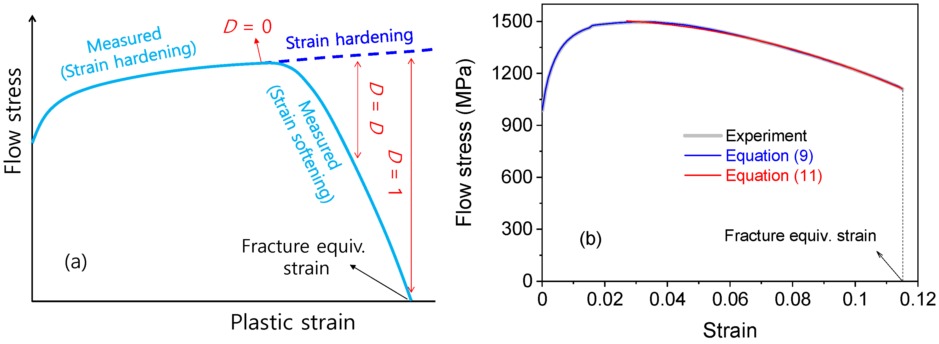
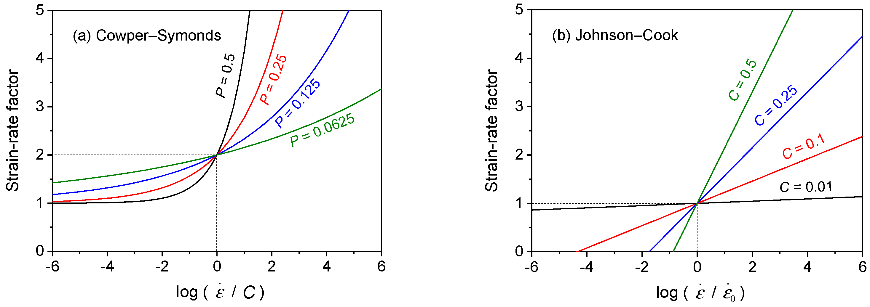
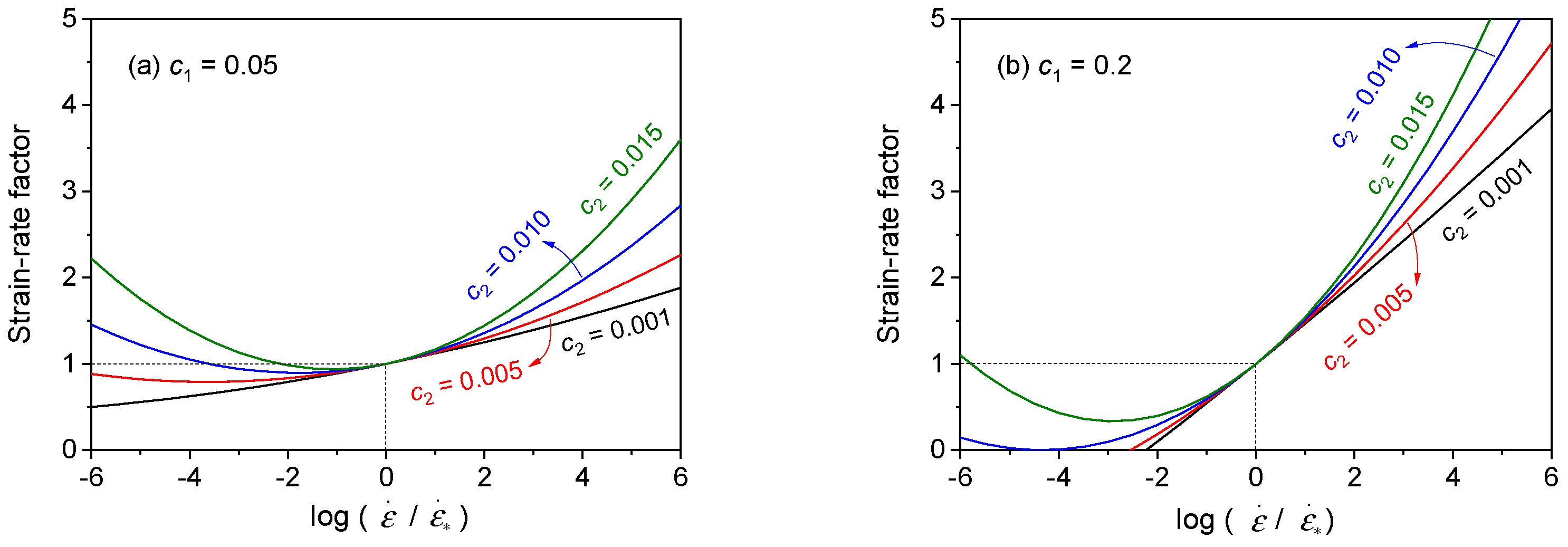
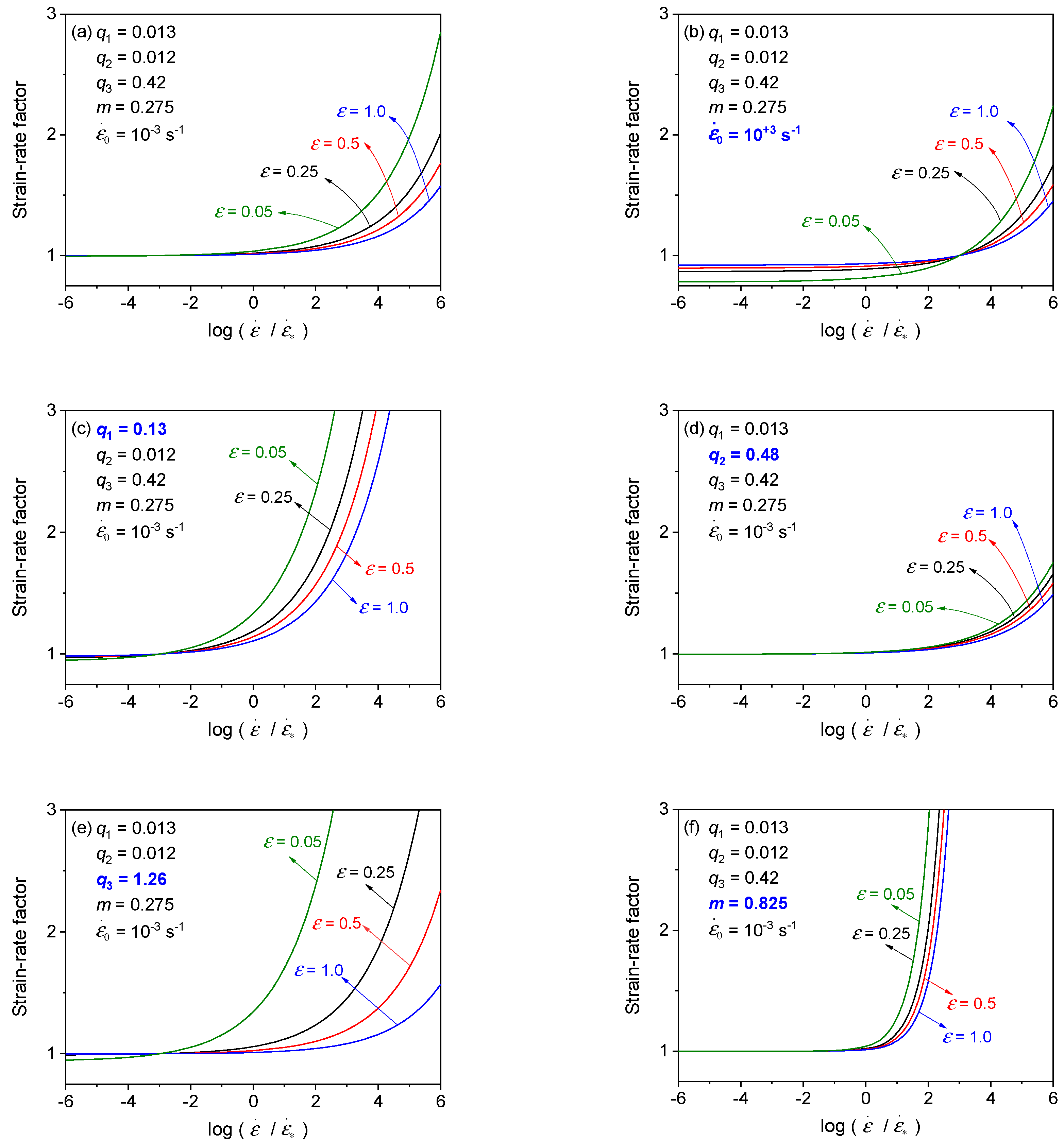
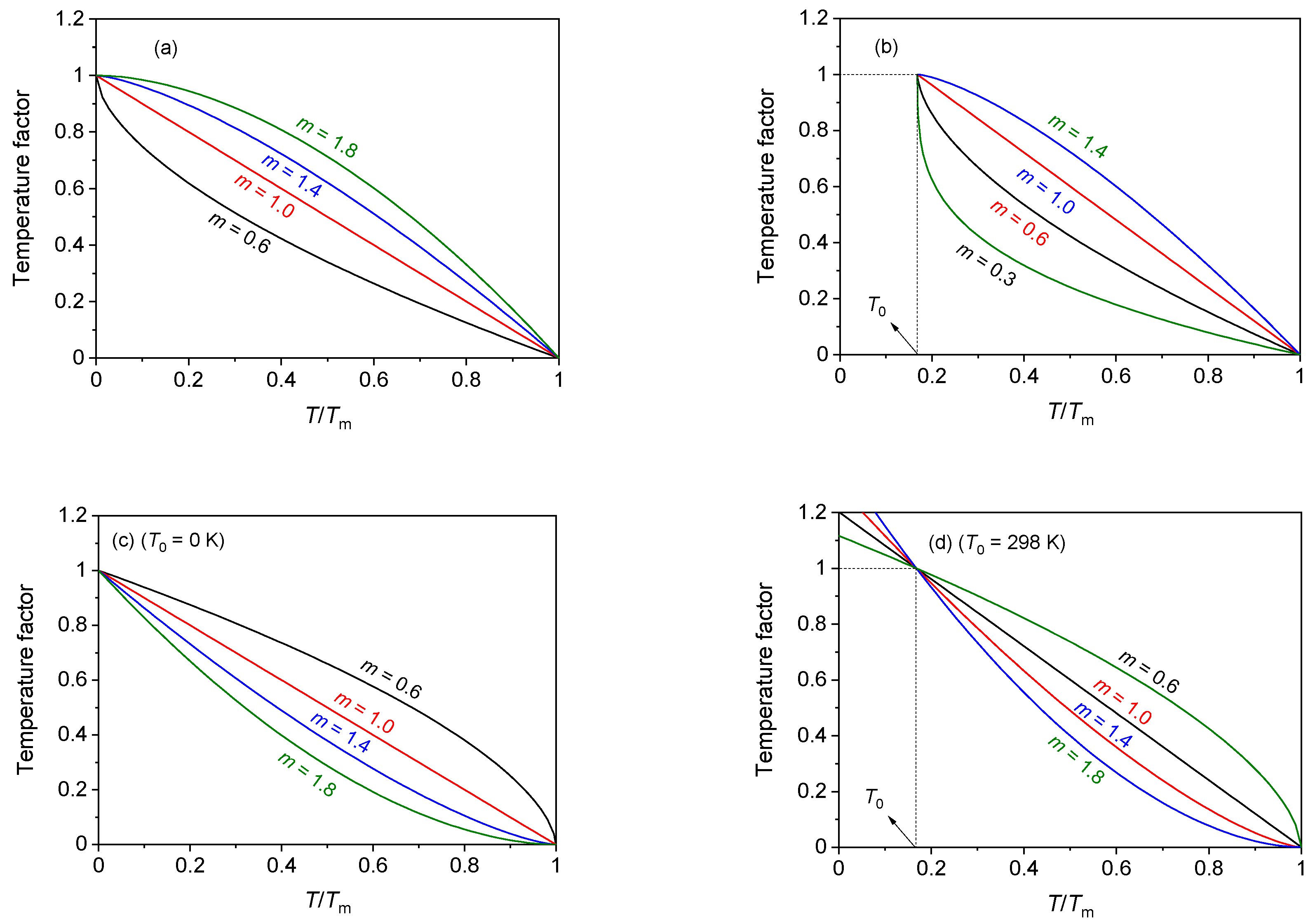
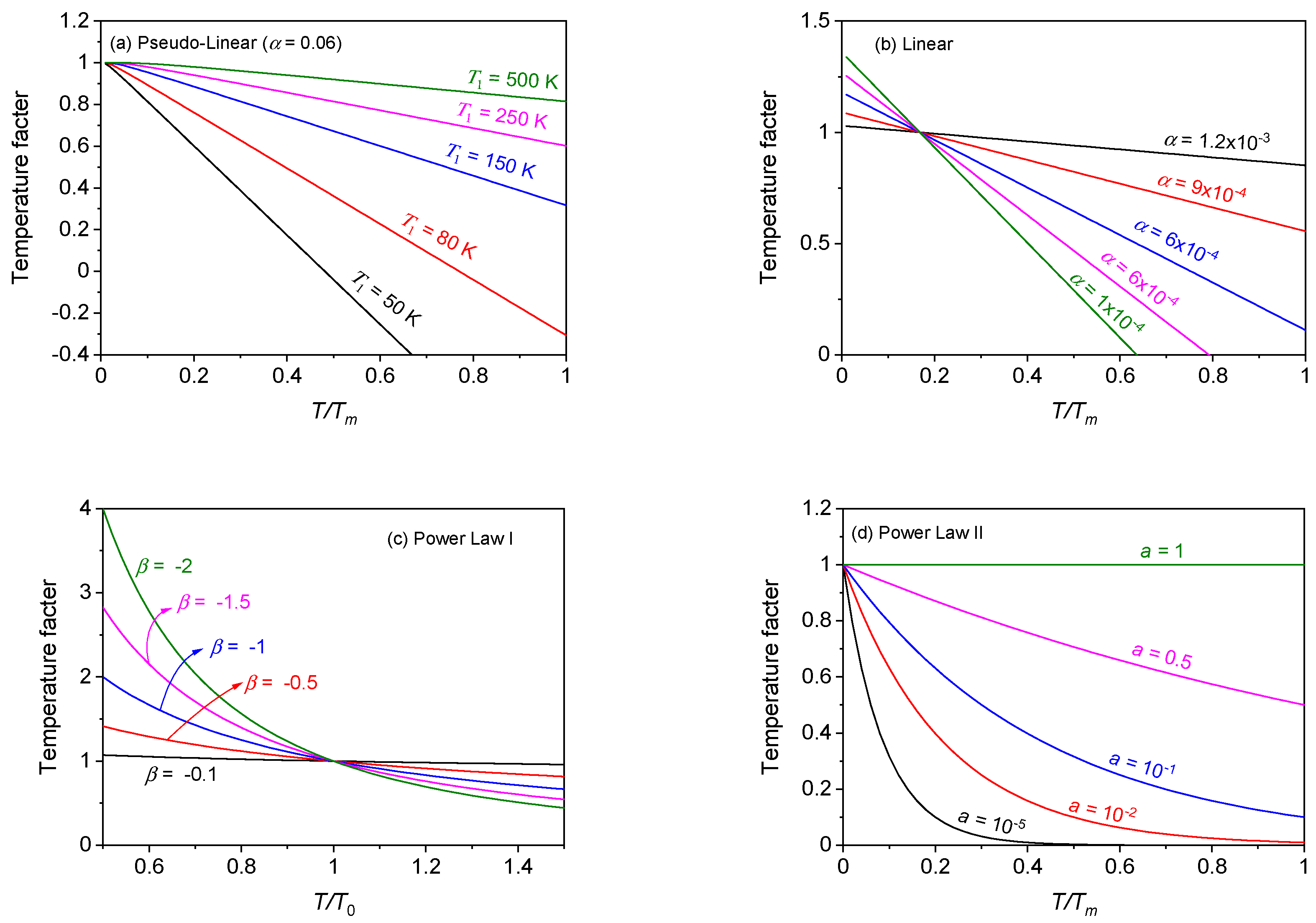
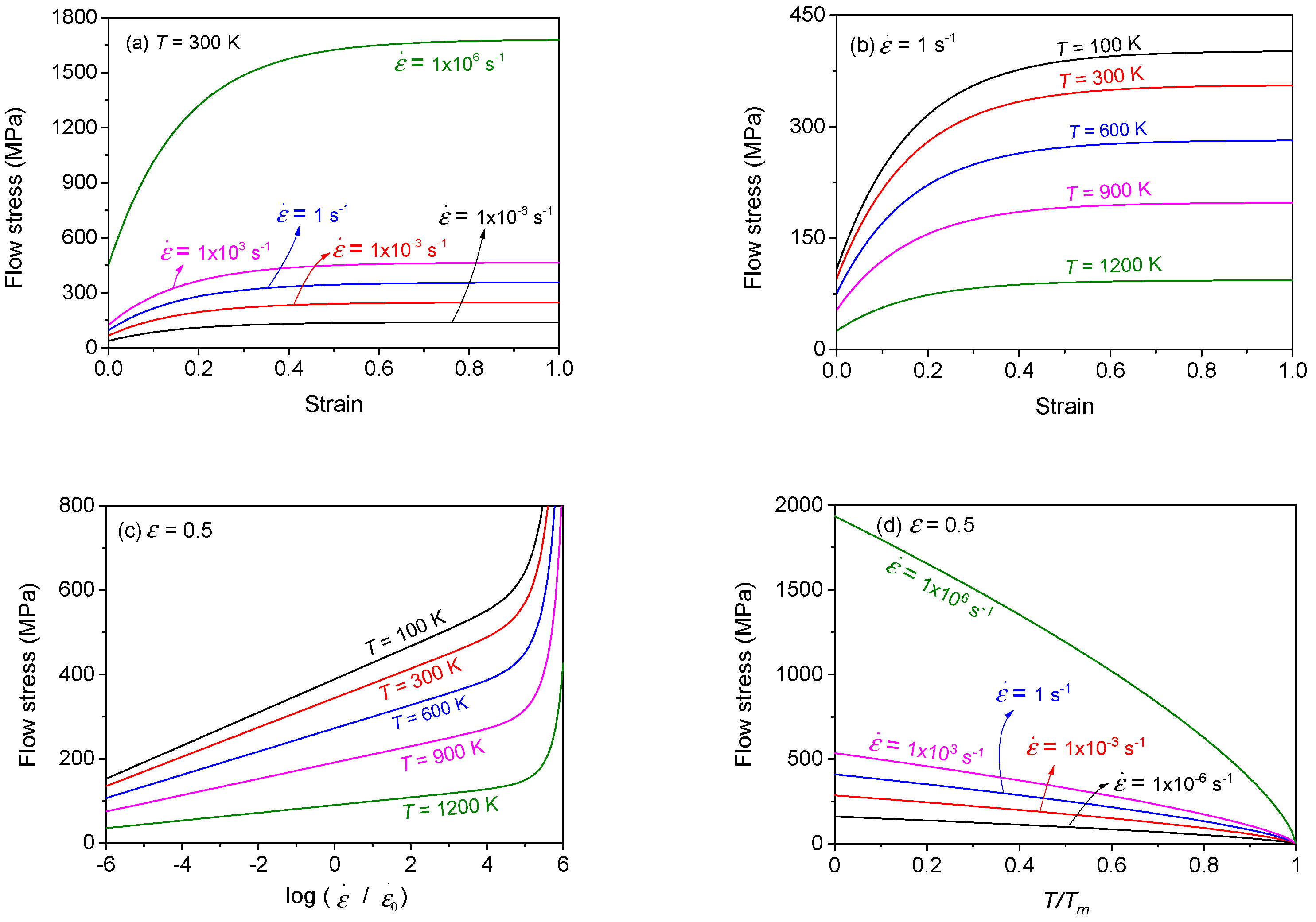
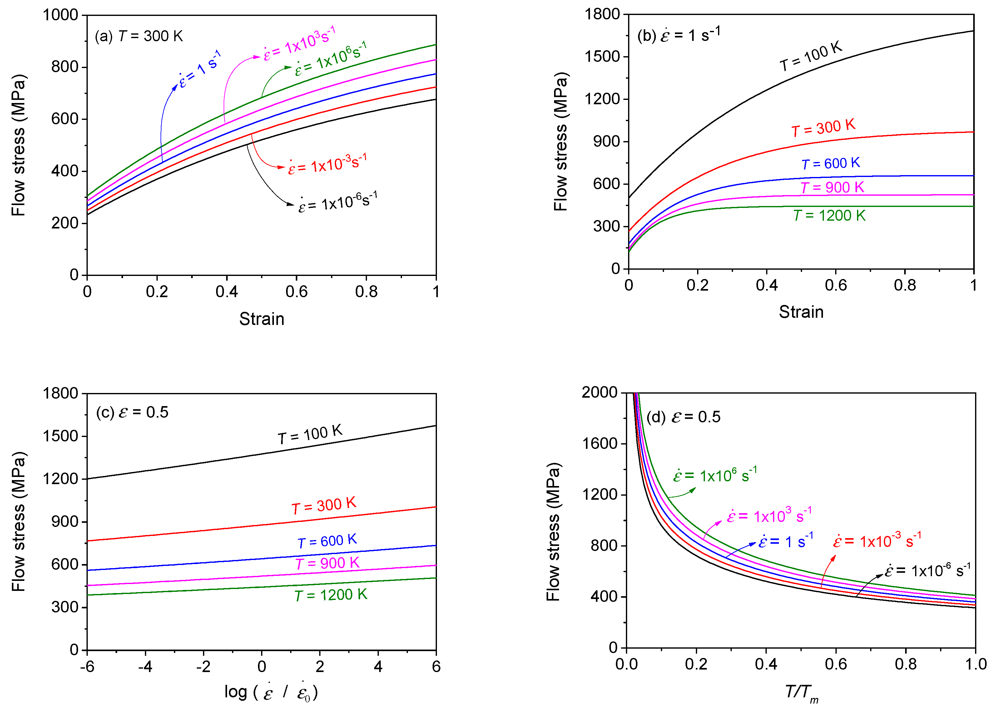
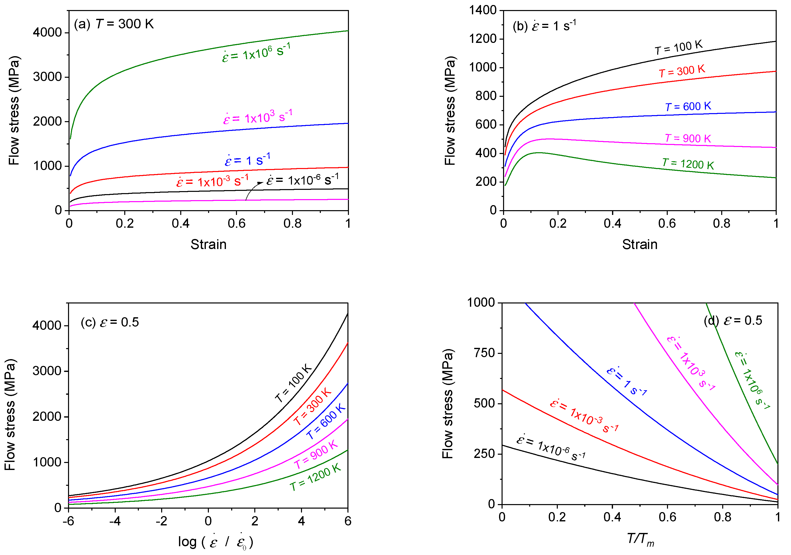
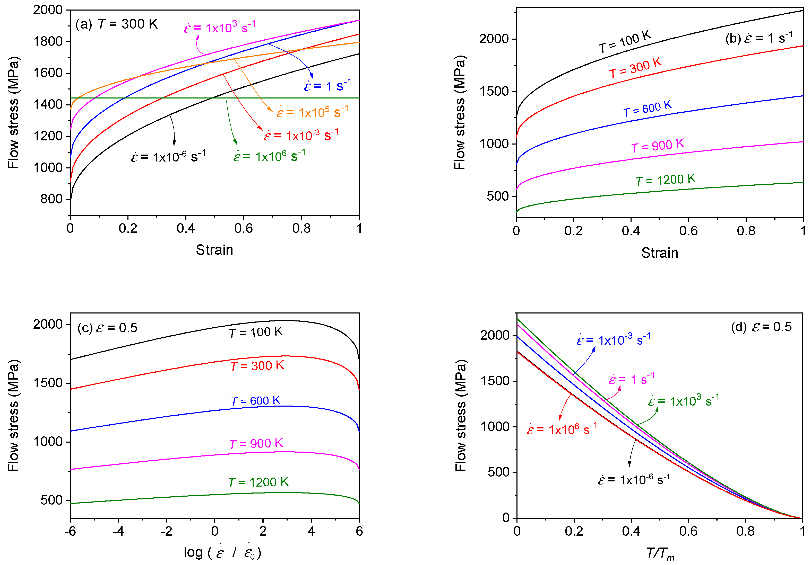
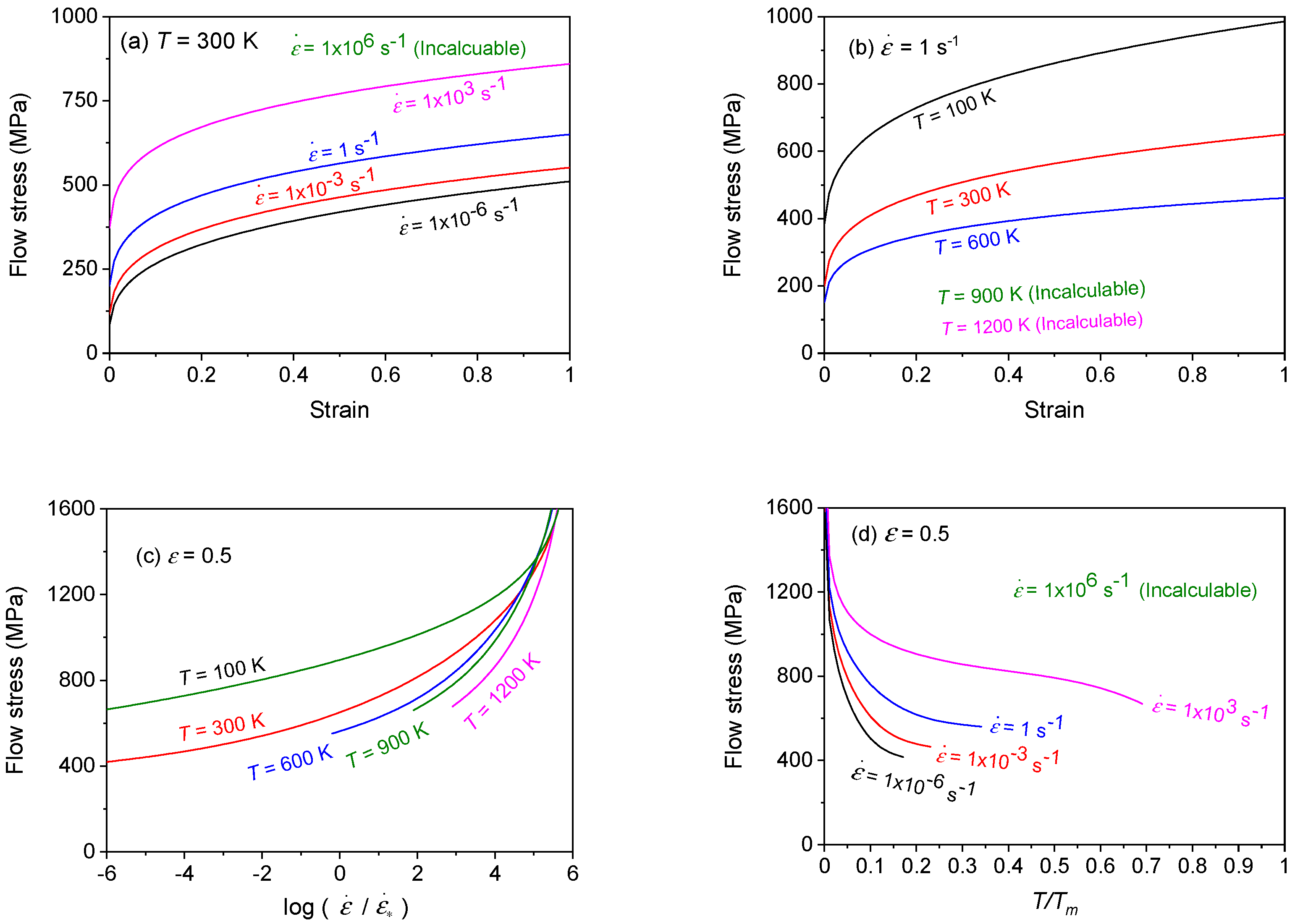
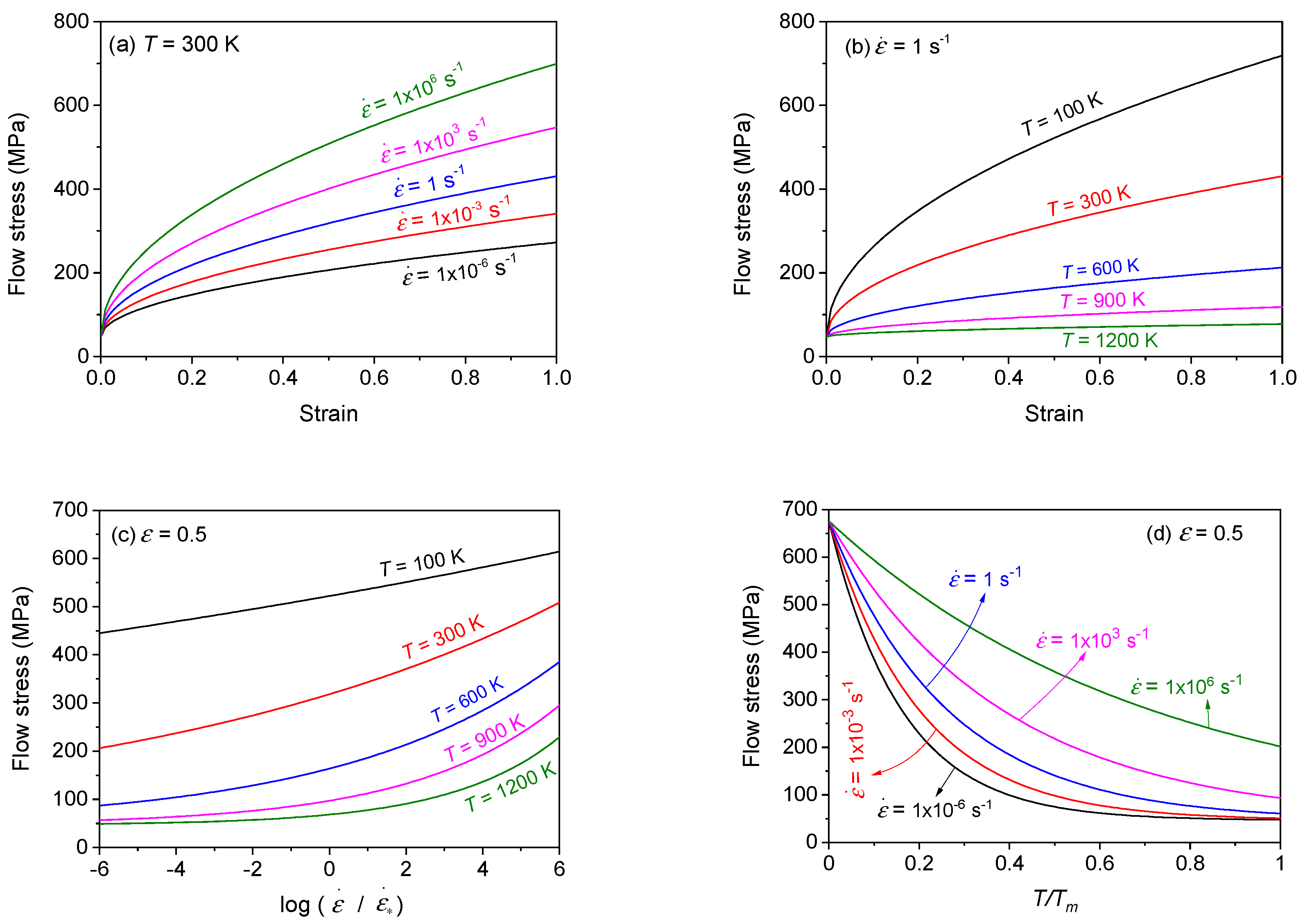
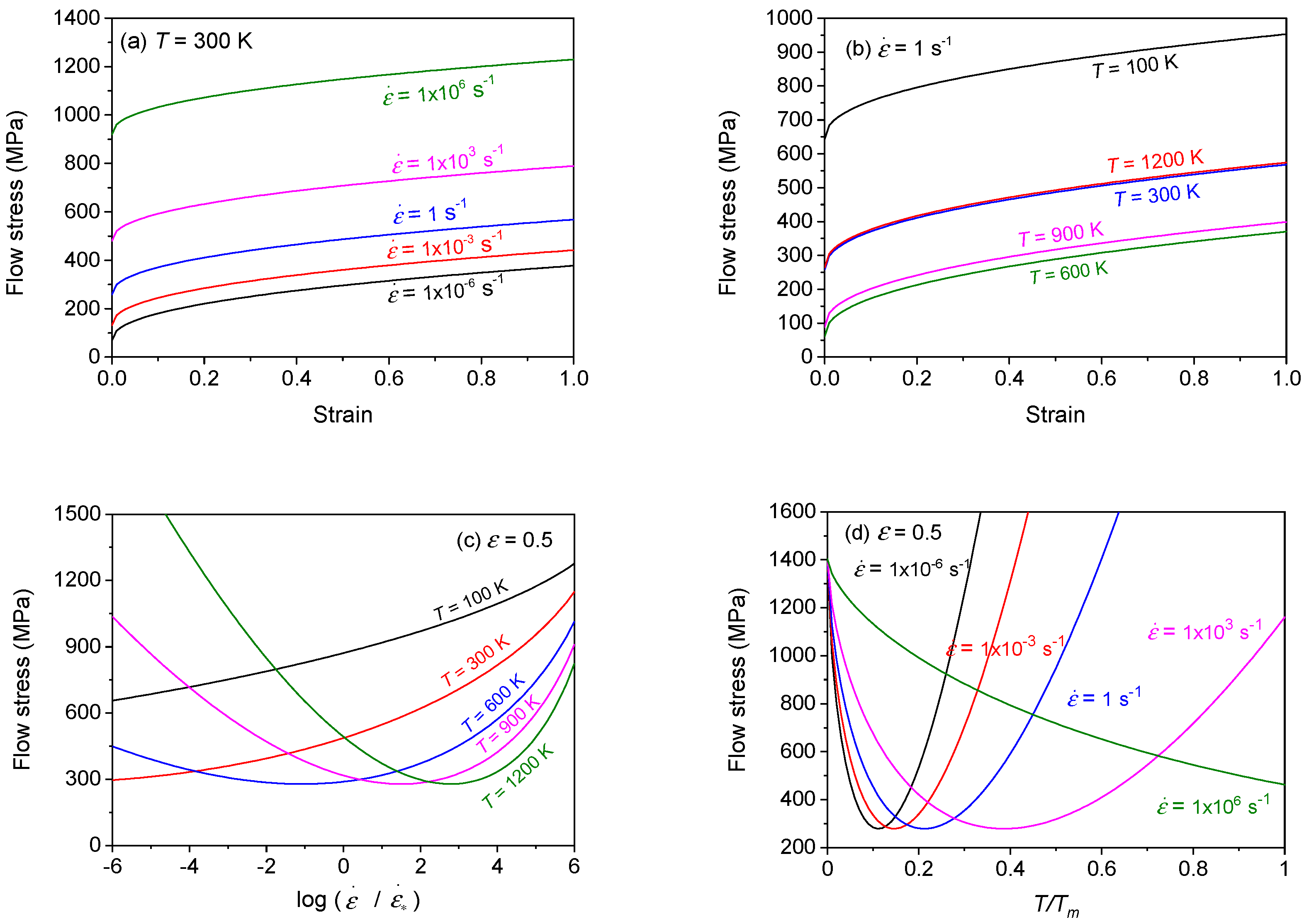
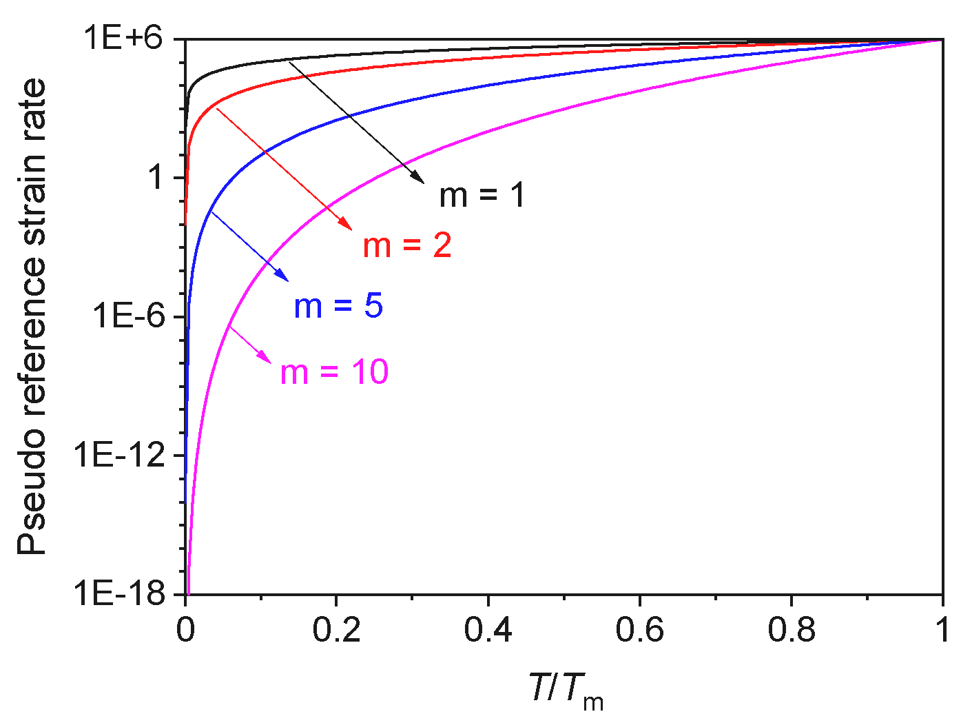
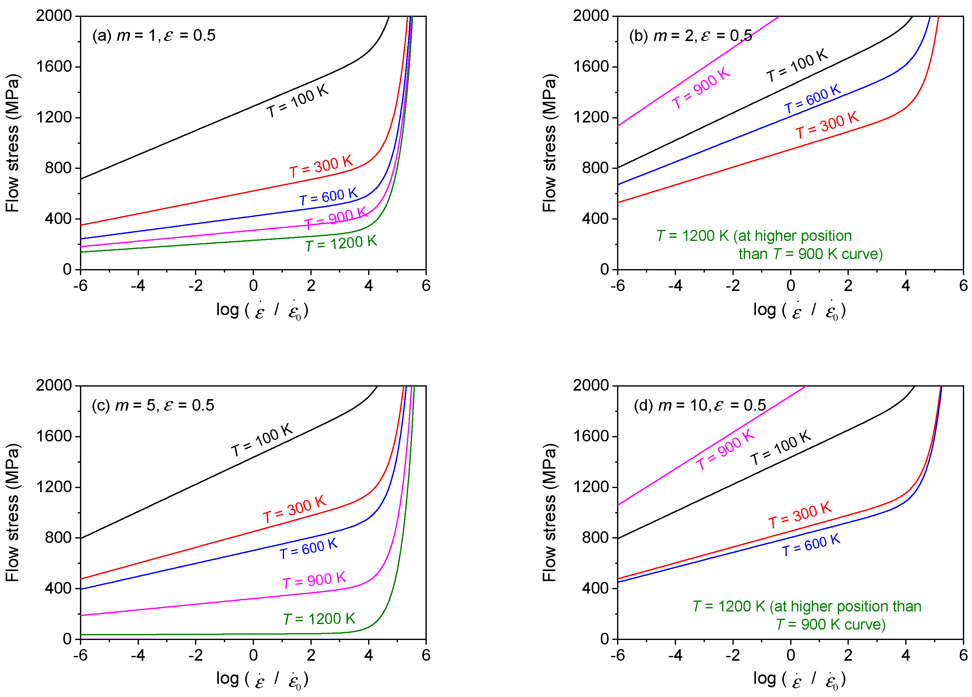
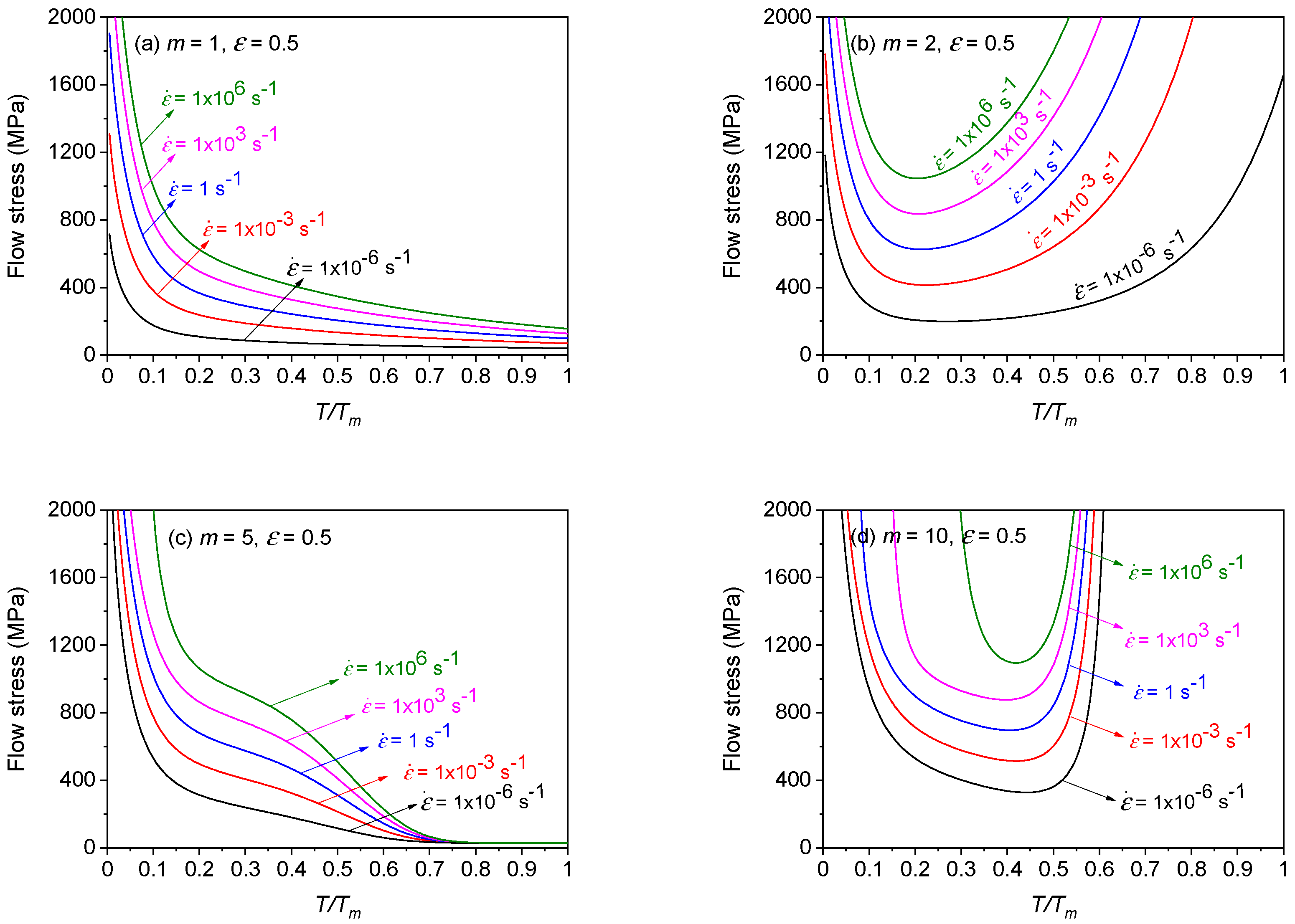
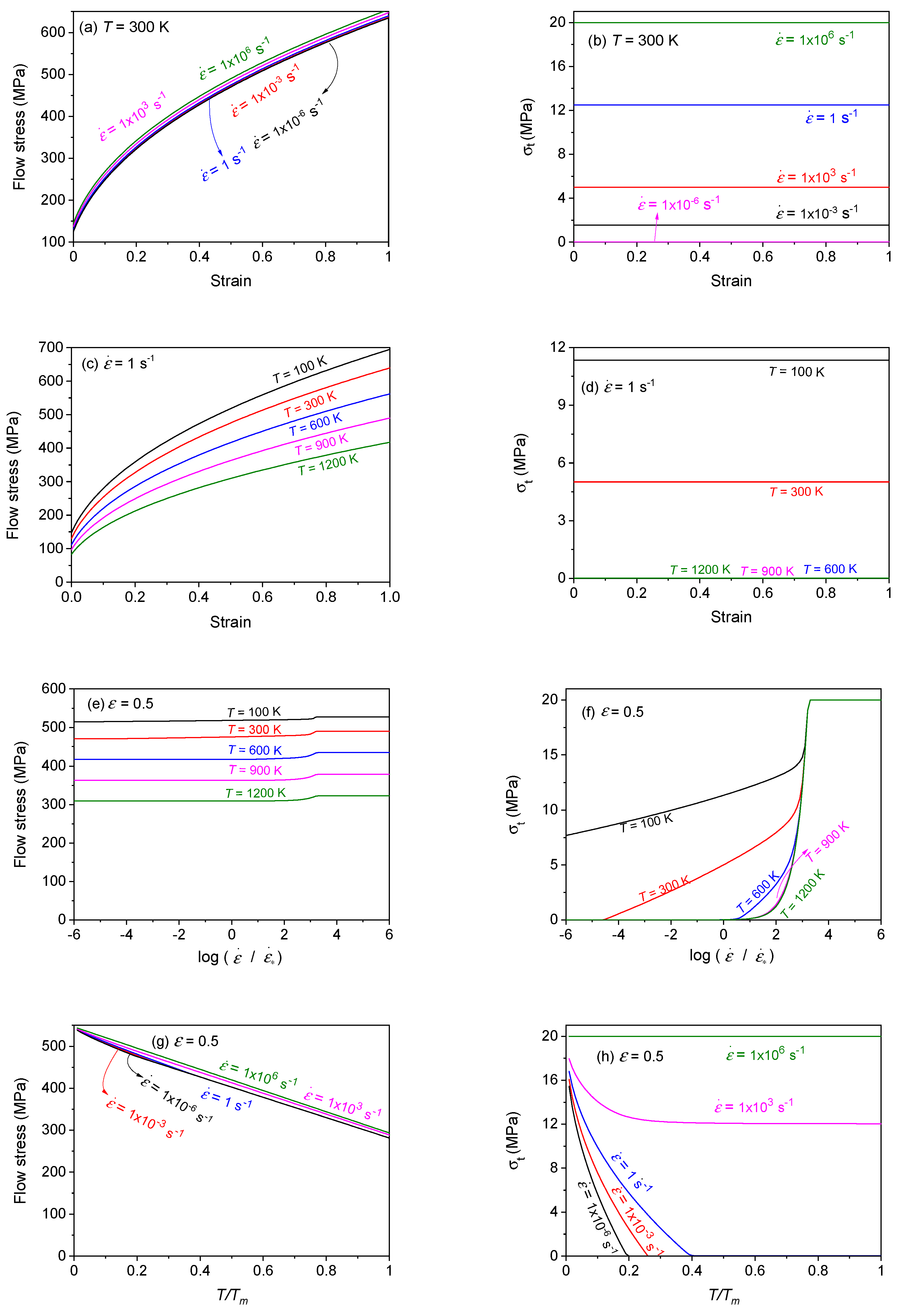
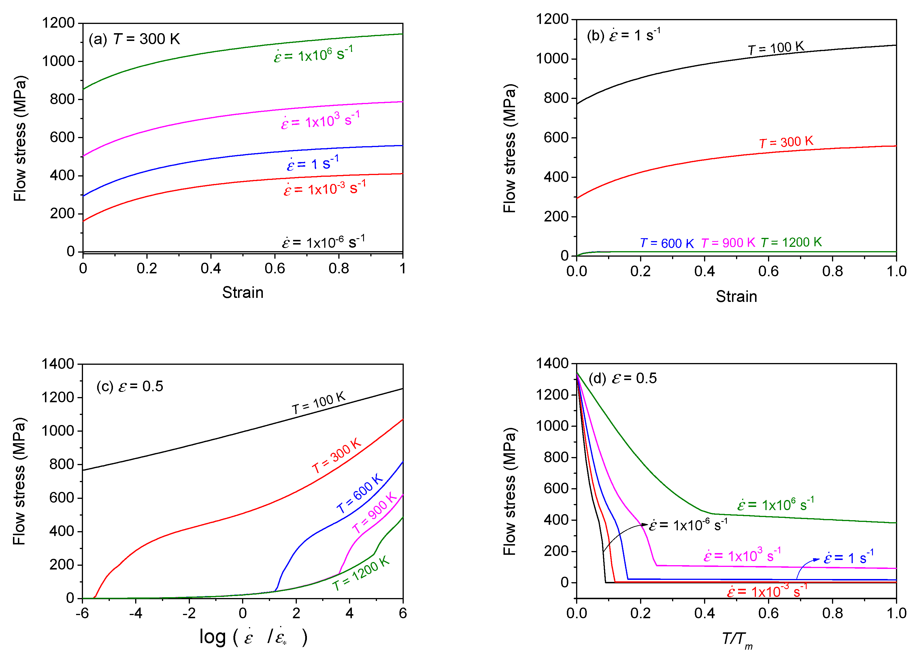
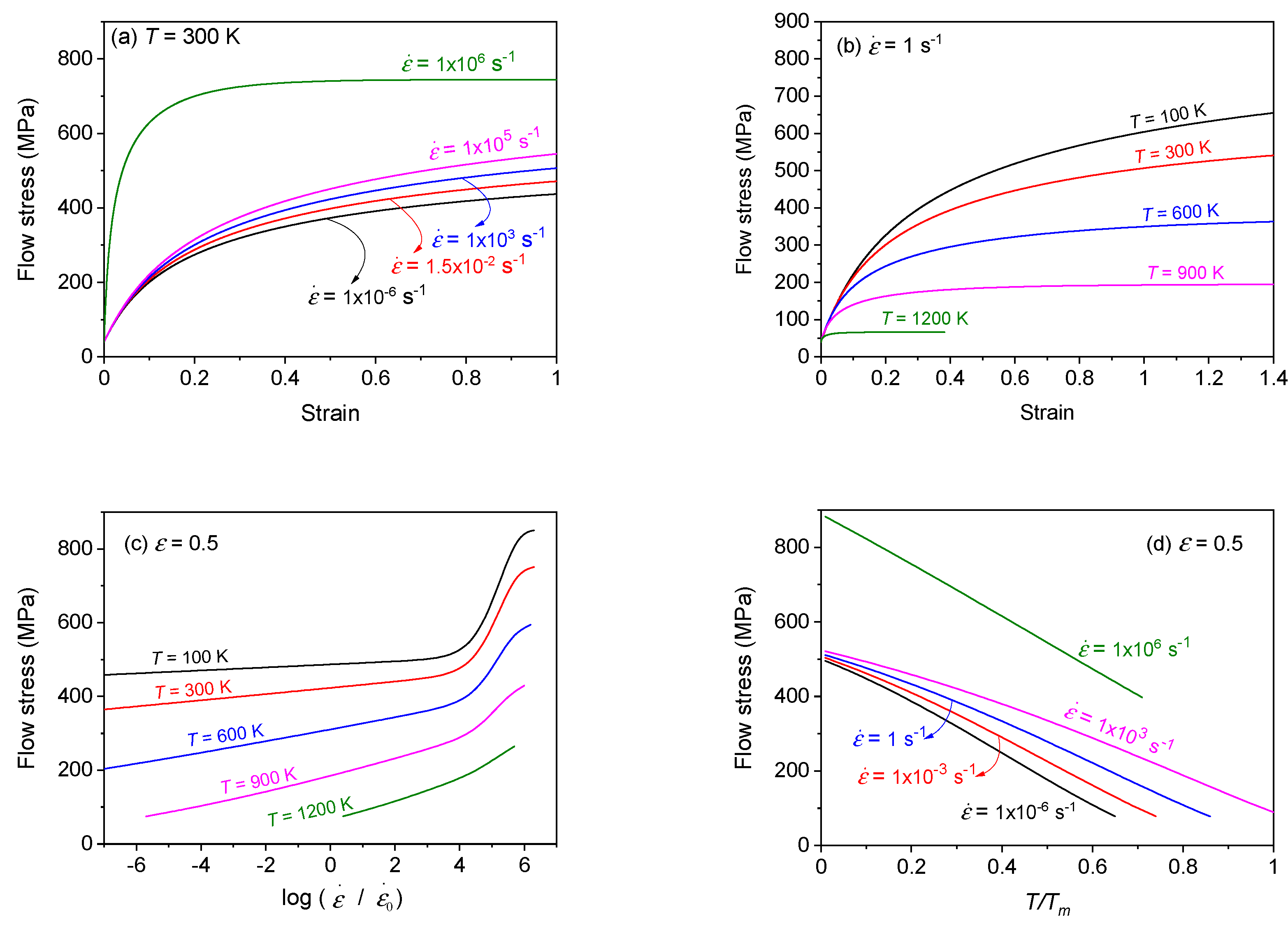
Table 1.
Parameters of the JC model for OFHC [10] (
= 1 s−1,
= 298 K, and Tm = 1356 K).
Table 1.
Parameters of the JC model for OFHC [10] (
= 1 s−1,
= 298 K, and Tm = 1356 K).
| Parameter | A | B | n | C | m |
| Unit | MPa | MPa | 1 | 1 | 1 |
| Value | 90 | 292 | 0.31 | 0.025 | 1.07 |
Table 2.
Parameters of the SK model for OFHC [70] (
= 1 s−1,
= 298 K, and Tm = 1356 K).
Table 2.
Parameters of the SK model for OFHC [70] (
= 1 s−1,
= 298 K, and Tm = 1356 K).
| Parameter | A | B | C | D | E | m |
| Unit | MPa | MPa | 1 | 1 | 1 | 1 |
| Value | 96 | 261 | 6.13 | 0.044 | 1.41 × 10⁻⁶ | 0.7 |
Table 3.
Parameters of the LW model for SS310 (
= 0.002,
= 298 K, and Tm = 1727 K) [12].
Table 3.
Parameters of the LW model for SS310 (
= 0.002,
= 298 K, and Tm = 1727 K) [12].
| Parameters | A | C | D | m | ||
| Unit | MPa | MPa | 1 | K−1 | 1 | 1 |
| Value | 989.3 | 0.7287 | −3.791 | −0.0086 | 0.0098 | −0.574 |
Table 4.
Parameters of the SKW model for DP590 steel (
= 1 s−1,
= 1 s−1,
= 298 K, and Tm = 1750 K) [13].
Table 4.
Parameters of the SKW model for DP590 steel (
= 1 s−1,
= 1 s−1,
= 298 K, and Tm = 1750 K) [13].
| Parameters | H | n | V | A | B | |||||
| Unit | MPa | 1 | MPa | 1 | 1 | 1 | K−1 | K−1 | 1 | 1 |
| Value | 1051 | 0.179 | 643.9 | 0.576 | 22.44 | 0.818 | 0.00193 | 2.7 × 10⁻⁴ | 0.001 | 0.1 |
Table 5.
Parameters of the KHL model for Ti–6Al–4V (
= 1 s−1,
= 106 s−1,
= 296 K, and Tm = 1933 K) [14].
Table 5.
Parameters of the KHL model for Ti–6Al–4V (
= 1 s−1,
= 106 s−1,
= 296 K, and Tm = 1933 K) [14].
| Parameters | A | B | n1 | n0 | C | m |
| Unit | MPa | MPa | 1 | 1 | 1 | 1 |
| Value | 1069 | 874.8 | 0.5456 | 0.4987 | 0.02204 | 1.3916 |
Table 6.
Parameters of the RK model for mild steel ES (
= 10−6 s−1,
= 106 s−1, and Tm = 1793 K) [16].
Table 6.
Parameters of the RK model for mild steel ES (
= 10−6 s−1,
= 106 s−1, and Tm = 1793 K) [16].
| Parameter | |||||||||
| Unit | 1 | 1 | MPa | 1 | 1 | 1 | MPa | 1 | 1 |
| Value | 0.0018 | 0.59 | 591.6 | 0.2 | 0.285 | 0.19 | 406.3 | 0.48 | 2.8 |
Table 7.
Parameters of the ZA model for an FCC material (copper) (
= 1 s−1,
= 1356 K) [17].
Table 7.
Parameters of the ZA model for an FCC material (copper) (
= 1 s−1,
= 1356 K) [17].
| Parameters | C0 | C2 | C3 | C4 |
| Unit | MPa | MPa | K−1 | K−1 s−1 |
| Value | 46.5 | 890 | 0.0028 | 0.000128 |
Table 8.
Parameters of the ZA model for a BCC material (tantalum) ( = 1 s−1, Tm = 3290 K) [18].
Table 8.
Parameters of the ZA model for a BCC material (tantalum) ( = 1 s−1, Tm = 3290 K) [18].
| Parameters | C0 | C1 | C3 | C4 | C5 | n |
| Unit | MPa | MPa | K−1 | K−1 s−1 | MPa | 1 |
| Value | 30 | 1125 | 0.00535 | 0.000327 | 310 | 0.44 |
Table 9.
Parameters of the VA model for tantalum ( = 1 s−1, Tm = 3290 K) [19].
Table 9.
Parameters of the VA model for tantalum ( = 1 s−1, Tm = 3290 K) [19].
| Parameters | B | n | q | p | ||||
| Unit | MPa | MPa | 1 | MPa | K−1 | K−1 | 1 | 1 |
| Value | 50 | 310 | 0.44 | 1125 | 0.0014343 | 0.0000937 | 1.5 | 0.5 |
Table 10.
Parameters of the TBRI model for A508 steel [20].
Table 10.
Parameters of the TBRI model for A508 steel [20].
| Parameters | A | T1 | T2 | m | Tm | |||||
| Unit | MPa | MPa | 1 | K | K | 1 | 1 | K | s−1 | MPa |
| Value | 28.7 | 407.0 | 2.7 | 86.5 | 908.5 | 9.83 | 0.033 | 1623 | 106 | 0.005 |
Table 11.
Parameters of the SCGL model for copper [22] (Tm = 1356 K).
Table 11.
Parameters of the SCGL model for copper [22] (Tm = 1356 K).
| Parameter | ||||||
| Unit | MPa | MPa | 1 | 1 | 1 | MPa |
| Value | 125 | 640 | 36 | 0.0 | 0.45 | 20 |
| Parameter | Uk | C1 | C2 | |||
| Unit | eV | s−1 | MPa·s | MPa | MPa·K−1 | 1 |
| Unit | 0.31 | 0.71 × 10⁶ | 0.012 | 47,700 | −18.126 | 0 |
Table 12.
Parameters of the PTW model for tantalum (Tm = 3290 K) [24].
Table 12.
Parameters of the PTW model for tantalum (Tm = 3290 K) [24].
| Parameter | θ | p | ||||||
| Unit | 1 | 1 | 1 | 1 | 1 | 1 | 1 | 1 |
| Value | 0.00821 | 4 | 0.0129 | 0.00353 | 0.00923 | 0.00136 | 0.012 | 0.4 |
| Parameter | γ | β | α | ρ | M | Tm | ||
| Unit | 1 | 1 | 1 | 1 | GPa | kgm−3 | kg/atom | K |
| Value | 0.634 | 1.38 × 10⁵ | 0.23 | 0.23 | 72.2 | 16,600 | 3.00471 × 10⁻²⁵ | 3290 |
| Parameter | p | q | A | |||||
| Unit | MPa | 1 | 1 | 1 | 1 | s−1 | 1 | MPa |
| Value | 40 | 2/3 | 1 | 107 | 1.6 | 6.2 × 10¹⁰ | 0.312 | 900 |
| Parameter | b | α | ) | |||||
| Unit | nm | MPa | MPa | MPa·s | 1 | K | GPa | GPa |
| Unit | 0.249 | 2390 | 12 | 0.034 | 0.05848 | 165 | 51.3 | 3 |
Table 14.
Flow stress description characteristics of the considered constitutive models in terms of (i) the calculability of the model at wide and T, (ii) variable with either or T, (iii) exponential (nonlinear) increase in with (stress upturn), and (iv) admissible temperature softening. The symbols mean that the respective phenomenon is o: described; ∆: partially described; ×: not described.
| Type | Models | Calculability at Wide and T | Variable with Either or T | Exponential (Nonlinear) Increase in vs. Plot | Admissible T Softening | Number Fitting Parameters | Number of Material Constants |
|---|---|---|---|---|---|---|---|
| Phenomenological | JC | o | o | × | ∆ 1 | 5 | 1 |
| SK | o | o | o | o | 6 | 1 | |
| LW | o | o | × | × | 6 | 0 | |
| SKW | o | o | o | × | 10 | 0 | |
| KHL | o | o | × | o | 6 | 1 | |
| RK | × | o | × | × | 9 | 1 | |
| Physically based | ZA-FCC | o | × | o | × | 4 | 0 |
| ZA-BCC | o | o | o | × | 6 | 0 | |
| VA | o | o | × | × | 8 | 0 | |
| TBRI | × | o | × | × | 10 | 1 | |
| SCGL | o | o | × | × | 5 | 8 | |
| PTW | o | o | × | × | 11 | 5 | |
| FK | × | × | o | × | 14 | 1 |
1 incalculable at T < Tref (admissible T softening in limited T range). Abrupt softening for some m values near Tref.
Publisher’s Note: MDPI stays neutral with regard to jurisdictional claims in published maps and institutional affiliations. |
© 2022 by the authors. Licensee MDPI, Basel, Switzerland. This article is an open access article distributed under the terms and conditions of the Creative Commons Attribution (CC BY) license (https://creativecommons.org/licenses/by/4.0/).
Share and Cite
MDPI and ACS Style
Shin, H.; Ju, Y.; Choi, M.K.; Ha, D.H. Flow Stress Description Characteristics of Some Constitutive Models at Wide Strain Rates and Temperatures. Technologies 2022, 10, 52. https://0-doi-org.brum.beds.ac.uk/10.3390/technologies10020052
AMA Style
Shin H, Ju Y, Choi MK, Ha DH. Flow Stress Description Characteristics of Some Constitutive Models at Wide Strain Rates and Temperatures. Technologies. 2022; 10(2):52. https://0-doi-org.brum.beds.ac.uk/10.3390/technologies10020052
Chicago/Turabian StyleShin, Hyunho, Yongwon Ju, Min Kuk Choi, and Dong Ho Ha. 2022. "Flow Stress Description Characteristics of Some Constitutive Models at Wide Strain Rates and Temperatures" Technologies 10, no. 2: 52. https://0-doi-org.brum.beds.ac.uk/10.3390/technologies10020052
Note that from the first issue of 2016, this journal uses article numbers instead of page numbers. See further details here.