Article

Solving Dual-Channel Supply Chain Pricing Strategy Problem with Multi-Level Programming Based on Improved Simplified Swarm Optimization

Integration and Collaboration Laboratory, Department of Industrial Engineering and Engineering Management, National Tsing Hua University, Hsinchu 30013, Taiwan
*
Author to whom correspondence should be addressed.
Submission received: 20 May 2022 / Revised: 8 June 2022 / Accepted: 9 June 2022 / Published: 11 June 2022
(This article belongs to the Special Issue 10th Anniversary of Technologies—Recent Advances and Perspectives)

Abstract

:
With the evolution of the Internet and the introduction of third-party platforms, a diversified supply chain has gradually emerged. In contrast to the traditional single sales channel, companies can also increase their revenue by selling through multiple channels, such as dual-channel sales: adding a sales channel for direct sales through online third-party platforms. However, due to the complexity of the supply chain structure, previous studies have rarely discussed and analyzed the capital-constrained dual-channel supply chain model, which is more relevant to the actual situation. To solve more complex and realistic supply chain decision problems, this paper uses the concept of game theory to describe the pricing negotiation procedures among the capital-constrained manufacturers and other parties in the dual-channel supply chain by applying the Stackelberg game theory to describe the supply chain structure as a hierarchical multi-level mathematical model to solve the optimal pricing strategy for different financing options to achieve the common benefit of the supply chain. In this study, we propose a Multi-level Improved Simplified Swarm Optimization (MLiSSO) method, which uses the improved, simplified swarm optimization (iSSO) for the Multi-level Programming Problem (MLPP). It is applied to this pricing strategy model of the supply chain and experiments with three related MLPPs in the past studies to verify the effectiveness of the method. The results show that the MLiSSO algorithm is effective, qualitative, and stable and can be used to solve the pricing strategy problem for supply chain models; furthermore, the algorithm can also be applied to other MLPPs.

1. Introduction

Supply chain systems have been progressively diversifying besides conventional retailing manners. Nowadays, the increased competition and globalization of the market have become necessary for different individuals in the supply chain to cooperate to achieve mutual benefits. The competitions within the supply chain have catching researchers’ attention [1,2].
Supply chain management (SCM) handles the entire production flow of a good or service, which is a network that moves the product along from the suppliers of raw materials to those organizations that deal directly with users. In addition, due to the invention and growth of the internet, the prosperity of third-party platforms—online retailing, has gradually increased; companies can engage an additional sales channel in direct selling their products to customers and create various ways of sales to increase income. The appearance of multi-channel supply chain management issues is due to the rapid growth of e-commerce, which has led some manufacturers to sell their products online and increase their sales channels to remain competitive and increase the accessibility of their products. The increase in sales channels represents the complexity of their competition as well as coordination. The market demand is sensitive to the selling price set by the seller, so in a supply chain system, pricing strategy is a complex and tedious decision with numerous factors that affect it.
With all these buying and selling behaviors in business activities, many variables are considered by either the seller or the buyer. Each party is expected to achieve its desired benefit or goal in conducting the activity. Under this premise, the parties coordinate to reach a consensus and gain equilibrium through repeated communication for possible requests to achieve compromises. Therefore, replacing traditional corporate goals with overall value maximization through a holistic approach to the supply chain is a key issue for companies to consider nowadays. Decentralized decision-making occurs when there is a conflict between decision-makers. A hierarchical structure of decentralized decision-making should be carried out according to organizational departments. The objectives of the decision-makers are independent, and they are aimed at maximizing their own profits.
In reality, however, the situation is actually not that simple. There may be some conflict of interest because the asymmetry of the market position causes an asymmetry in the order of decision making for this German economist Heinrich Freiherr von Stackelberg proposed the Stackelberg model in 1934 to describe this situation of priority order decision making with leaders and followers [3]. In addition, the equilibrium point of this problem is determined through the solution of the Stackelberg game. The Nash equilibrium does not guarantee the best resolution for all decision-makers, the result may not be the most favorable situation, but it is an acceptable outcome for all parties. As a result, some studies use the method of multi-level programming (MLP), a mathematical model for solving decentralized decision-making problems, as an extension of the Stackelberg game to find the solution [4,5,6]. The key feature of this model is that the decision-makers have independent objective functions at each level of the hierarchy and control over the selection of decision variables.
The earliest proofs that a multi-level programming problem (MLPP) is an NP-hard problem are Ben & Blair (1990) [7] and Bard (1991) [8], and the bi-level programming problem (BLPP) they solved and proposed is derived from the MLPP problem, so the more complex MLPP also belongs to the NP-hard problem. Because of its limitations and complexity, it is more difficult to solve large-scale problems by mathematical planning methods. In recent years, researchers have adopted the more efficient meta-heuristic algorithm to obtain approximate solutions [6,9,10,11,12], which may not always lead to the best solution, but can handle more complex MLPP problems.
Nowadays, with increasingly complex supply chain relationships, companies need to be equipped with better decision models to manage their own goals. These problems can be solved by proposing suitable algorithms that can solve MLPP in a reasonable time and, at the same time, obtain an acceptable quality of the solution. The relationship between the supply chain network and the logistics distribution scheduling as regards applying swarm optimization algorithms proposed by some scholars, they harnessed the machine learning method, algorithms in the retailing environment in dynamic assessment to determine the users’ trends and patterns and grasp customer attitudes and feelings [13,14,15,16].The improved Simplified Swarm Optimization (iSSO) designed by Yeh [17] in 2015 is one of the evolutionary algorithms and stochastic optimization algorithms. It is characterized by the simplicity and efficiency of the iterative method. The algorithm demonstrates its excellent efficiency and generates high-quality solutions in solving most of the continuity problems.
Based on the above-mentioned excellent features, we propose an approach that uses iSSO to further optimize the pricing strategy by constructing an MLPP model that can effectively maximize the profit among all parties.
The purpose of this study is to investigate the use of an MLPP to solve the pricing problem of the supply chain, considering the financing decision options under dual sales channels where different options generate different interactions among the parties in the supply chain that will affect the pricing strategy. Therefore, this paper first uses the study of Zhen (2020) [18] as the basis of the mathematical model of a dual-channel supply chain system to analyze the profit formula of each party under different financing strategies.
This study aims to develop a method to solve the NP-hard problem of MLPP and construct and investigate the multi-level supply chain system by exploring how the decision-makers in the supply chain system should decide on the best pricing strategy to maximize the profit. By considering various competing influences, the benefits of the supply chain system are maximized by making pricing decisions that satisfy all parties. Thus, the ideal situation is to prioritize the manufacturer’s best interests and minimize the costs of all parties while achieving the best interests of the other parties.
The study objectives can be summarized as follows,
  • Build an MLPP model to obtain the equilibrium solution of pricing strategy in the dual-channel supply chain system.
  • Study and analyze the best decision for the manufacturer on finance strategy.
  • Apply the improved, simplified swarm optimization algorithm to multi-level programming problems.
The rest of this article is organized as follows. Section 2 lists the theoretical basis of the research. Section 3 describes the supply chain model, including proposed symbols, assumptions, and mathematical models. In Section 4, we introduce the research method, including the concept of MLPP and iSSO, and discuss the novelty and steps of the proposed MLiSSO. In Section 5, we analyzed the effects of the proposed method and described in detail the results of the above-mentioned supply chain pricing strategy. Finally, our conclusions are given in Section 6.

2. Literature Review

2.1. Dual-Channel Supply Chain

Nowadays, due to the rapid development of technology, various sales models have emerged in our society. In response to the purchasing habits of the new generation, the development of online retailing has become more and more prevalent.
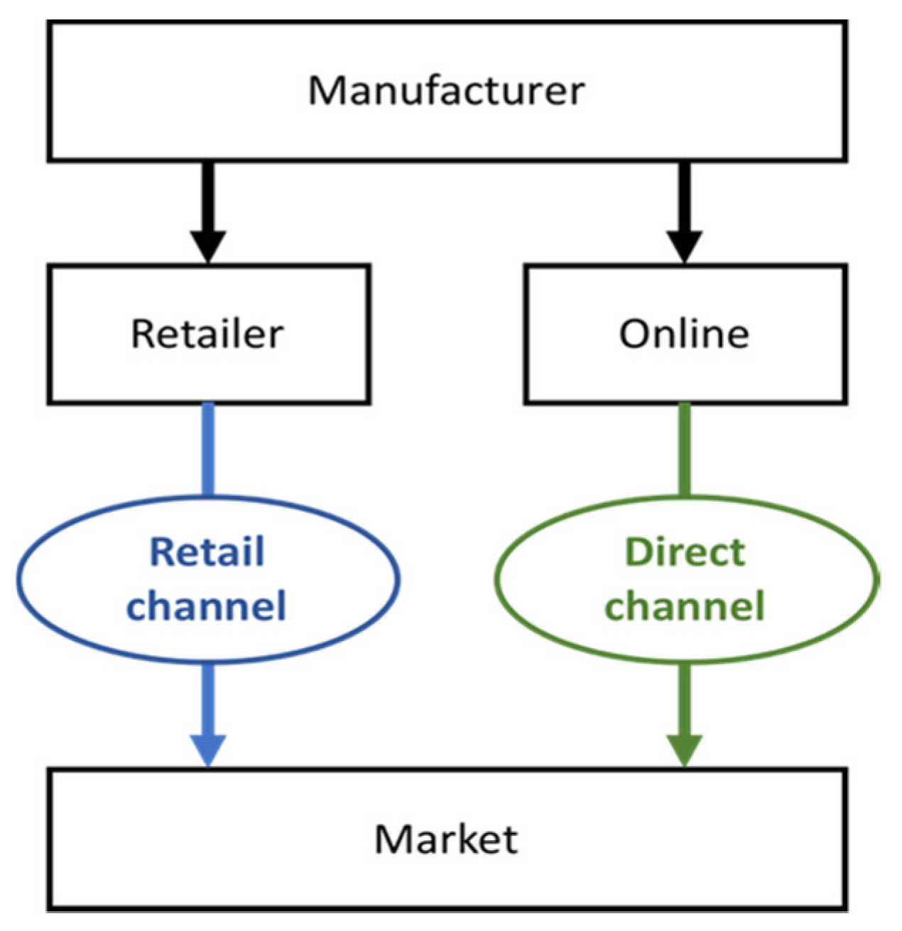
In addition to traditional sales channels, upstream manufacturers in the supply chain are gradually developing channels to sell their products directly online. In this way, sales can be managed through a third-party platform without expanding your physical store or website and only require the costs associated with the platform, such as profit sharing and rent; the structure of the dual-supply chain is shown in Figure 1. Various studies on the supply chain phenomenon are also available in the market with service competition [19], channel selection [20], pricing strategies [21], and dual-channel supply chains [22].
Channel competition holds an important role in dual-channel supply chain management. For example, Bernstein et al. (2009) address how competition between both retail and direct channels affects decisions made by manufacturers on supply chain structure [23]. Ryan et al. (2012) discussed the price competition and coordination in a dual-channel model [24]. Saha (2016) compared the performance of the manufacturer, the distributor, the retailer, and the entire supply chain in three different supply chain structures to prove that under some conditions that a dual-channel can outperform a single retail channel [25].
However, the studies on dual-channel supply chains mostly do not assume that firms are capital constrained; therefore, this study uses the financing strategy preferences of capital-constrained firms in the dual-channel supply chain proposed by Zhen in 2020 [18] while considering the financing strategies of third-party platforms in SCM. As a result, this study considers the operational management and financing strategy preferences of supply chain systems in the above-mentioned points.
Therefore, based on the model proposed by Zhen [18], this study examines the two aforementioned financing approaches for dual-channel competition and consumer considerations and presents the decision relationships between manufacturers and retailers with three different financing strategies. In addition, we compare the impact of cost and revenue on manufacturers, retailers, and lenders in the supply chain, maximizing profit and minimizing each cost to obtain the best pricing decision for the entire supply chain.

2.2. Supply Chain Finance

As the members of the supply chain gain benefits by selling their products while the market demand is sensitive to the selling price of the products, therefore, the pricing decision plays an important role in the profit optimization of the supply chain [6]. In considering changes in the correlation between product prices and market demand, companies can make profit analysis and pricing strategies efforts [26].
Lack of funding may be a hindrance to business development. There are two types of financing discussed in the literature on supply chain financing. One type of financing is external financing, which is defined as loans from institutions outside the supply chain, such as banks, third-party logistics, or other financial institutions. The other is internal financing, defined as loans from companies in the supply chain to their upstream or downstream companies, such as trade credit and buyer’s credit [27].
Most research on internal financing has examined trade credit financing, with the majority of studies focusing on contract coordination and operational decisions under credit risk [28,29]. For external financing, the emphasis is on how the financing affects inventory or operations management and supply chain coordination [30,31]. Unlike the previous studies, Zhen (2020) focuses on the capital constraints of upstream firms under channel competition. This study is significant in examining how the capital constraints of upstream manufacturers affect the operation of dual channels [18].
When sales are not limited to traditional retail channels, to maximize the overall revenue is to develop a multi-channel pricing strategy, and it is cooperation and negotiation between each member in the supply chain system which can be considered as a game. For example, Matsui (2017) proposed that it would be appropriate for the manufacturer to release the direct selling price before the wholesale price is set. A sub-game perfect Nash equilibrium with the non-cooperative game of channel members is reached, and the manufacturer’s profit is maximized [1]. The subgame perfect Nash equilibrium of the non-cooperative game with channel members is reached, and the manufacturer’s profit is maximized.

2.3. Game Theory

Game theory is considered to be one of the most effective tools for dealing with these management problems. The well-known Prisoner’s Dilemma and the Nash Equilibrium of modern noncooperation have become important concepts in game theory.
The strategic interactions between players are what game theory studies as the real-life dilemma that we often encounter. A strategic interaction means that the optimal choices of one player depend on other players’ optimal choices and vice versa. Assume that each player is aware of the equilibrium strategies of the other players. In addition, none of the players gains any benefit by unilaterally changing its own strategy.
Increasingly, research papers are applying game theory to supply chain management [2,32,33]. Cachon and Zipkin [34] addressed the Nash equilibrium in a non-cooperative supply chain with one supplier and multiple retailers. Hennet and Arda [35] evaluated the efficiency of different types of contracts among industrial parties in a supply chain. Tian et al. [36] proposed a dynamic system model for green supply chain management based on evolutionary game theory, which applied game-theoretic methods to decision-making purposes.

2.4. Stackelberg Game

Several researchers have studied through game theory about coordination between manufacturers and retailers [37,38]. Each member attempts to maximize their own profit, a situation known as a non-cooperative game.
Since the market position asymmetry leads to the asymmetry of the decision sequence, there may be some conflict of interest. For this reason, the German economist Heinrich Freiherr von Stackelberg proposed the Stackelberg model in 1934 [3]. The Stackelberg model emphasizes the sequential relationship of decisions. In a game, the player who decides on a decision firstly is called the first player, while the other player is called the follower. When the first player decides his own strategy, he has already taken into account the possible decisions made by the followers in response to the first player’s decision. After the first player’s decision, the follower observes the first player’s decision and thinks about the effect of the strategy on itself, and then makes the best response decision. The whole process means that both sides in the game make decisions based on the pursuit of their own best goals while considering the possible best response of the other side.
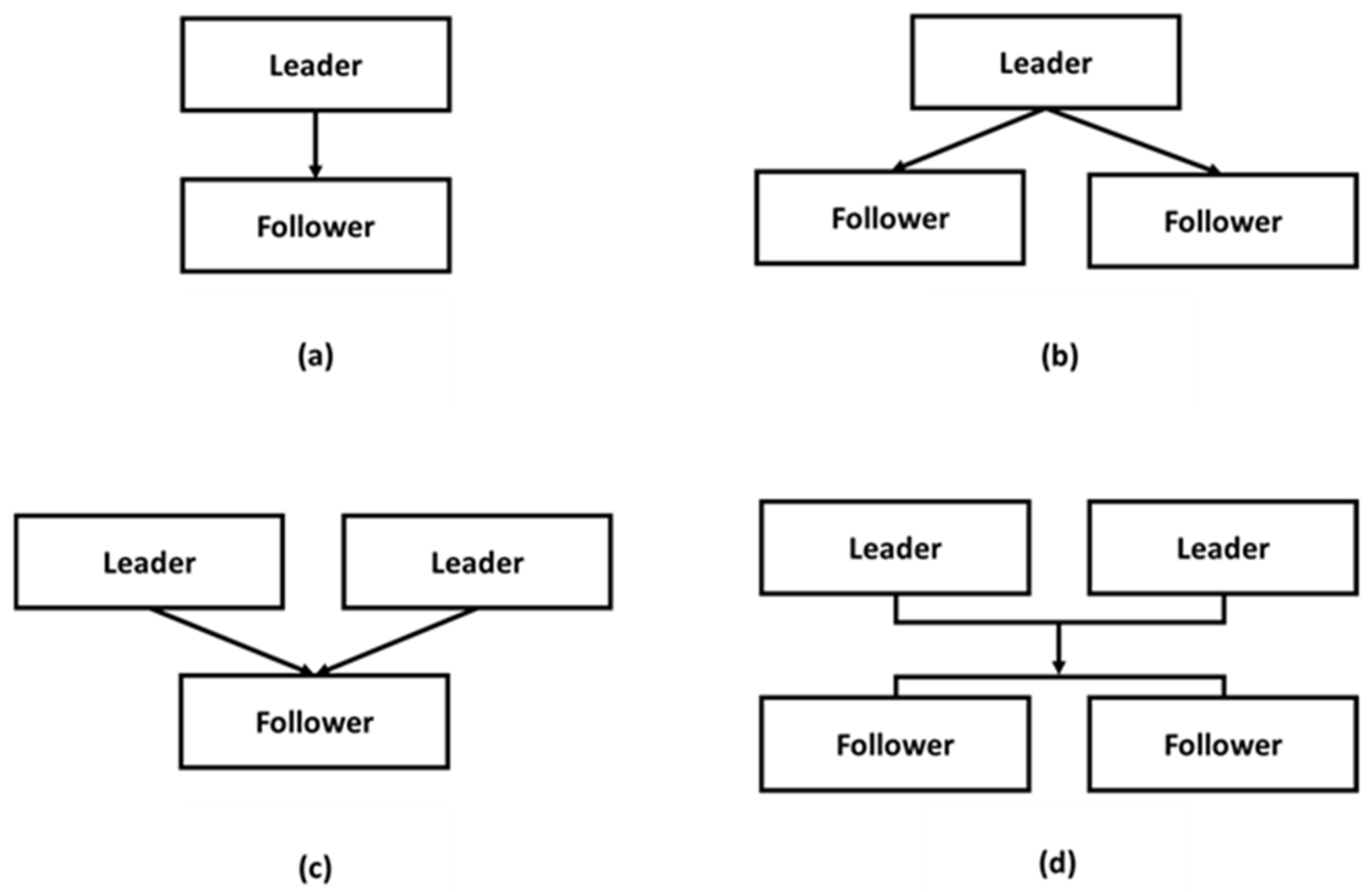
In the Stackelberg non-cooperative game, the dominant (leader) member controls the other members who act after the leader (followers). After estimating the reactions of other members, the leader will take the first decision [39]. The aforementioned hierarchical structure and the sequential nature of decision-making are consistent with the context set by Stackelberg’s theory. Therefore, the main modeling framework in this paper applies the Stackelberg model in the tournament.
According to the number of participants, the Stackelberg game can be divided into four main structures, as shown in Figure 2.

2.5. Multi-Level Programming Problem

In this section, we first review the development of techniques for solving the Stackelberg game problem, then addresses the general formulation of the bi-level programming problem model and multi-level programming problem model.
The multilevel programming problem (MLPP) is an extension of the Stackelberg game [39]. It aims to solve decentralized planning involving multiple decision-makers, where each member seeks to maximize its own interests in a hierarchical organization. This mathematical model has been widely used in practical problems such as resource allocation [4], transportation network design [5], and pricing and lot-sizing [6].
When decision-makers conflict with each other, a decentralized decision-making problem arises. The decentralized decision-making should be by organization departments and form a kind of hierarchical structure. The decision makers’ objectives are independent and may have some conflict of profit. Every decision-maker always wants to achieve a win-win situation called “dominant strategic equilibrium." However, in reality, the situation is actually not that simple. Nash equilibrium does not guarantee the best solution for every decision-maker, but it can get the best solution under the consideration of the entire group; therefore, multilevel programming (MLP) would be needed to find a solution. Zhou (2012) used game theory to determine the optimal pricing strategy to maximize the multilevel remanufacturing reverse supply chain [40]. Sadigh et al. (2012) found the optimal equilibrium of price, advertising spending, and production strategy in a bi-level programming approach [41].
The multilevel programming model has more advantages compared to the traditional single-level programming model. Its main benefits are (1) multilevel planning can be applied to analyze both different or even conflicting objectives in the decision process; (2) The multi-criteria approach of bi-level planning for decision-making can better reflect the actual problem; (3) The multi-level planning approach can denote the interactions between decision-makers.
In the current development of multi-level programming, several challenges emerge (1) Large scale—due to high dimensional decision variables for multi-level decision problems which become complex; (2) Uncertainty—with the uncertain information causing imprecise or unclear decision parameters and conditions for the decision subjects concerned; (3) Variety—with the possibility of the existence of multiple decision subjects with various relationships among them in each decision level. Yet, existing decision models or solution methods cannot fully and effectively handle these large-scale, uncertain and diverse multilevel decision problems [42].
There are two fundamental problems in solving MLPPs from a practical point of view. The first is the way to construct a multilevel decision model that describes the hierarchical decision process. Depending on the number of objectives involved, including dual objectives or multiple objectives; the number of members involved, including single leaders and followers or multiple leaders and followers; and the number of layers in the structure, including the bi-level programming problem (BLPP) or the MLPP. The BLPP is a special type of MLPP, and most of the research has been devoted to the BLPP study [9,10,11,41,43]. In addition, MLPP making that it is more complex than BLPP has been studied in depth in model building.
A further problem is how to identify methods for optimizing decisions. Several solving methods have been developed to solve these problems, broadly classified as exact algorithms and intelligent optimization algorithms. On the basis of the complexity of solving MLPP solutions, Ben & Blair (1990) proved through the well-known knapsack problem that BLPP is an NP-hard problem [7], and Bard (1991) even proved that BLPP is also an NP-hard problem through the search for locally optimal solutions [8]. This leads to exact algorithms that are time-consuming in solving nonlinear, discrete, and multi-optimal versions of large-scale problems that rely heavily on target function differentiability, which is not universally applicable [42].
At present, to obtain the optimal solution of MLPP, metaheuristic algorithms or innovative computations have been designed and widely used to solve BLPP and MLPP, i.e., Liu (1998) proposed a genetic algorithm for solving the Stackelberg-Nash equilibrium problem for generic MLPP with multiple followers [12], and Ma et al. (2013) using Particle Swarm Optimization (PSO) to solve BLPP on supply chain model [6]. Moreover, extending these algorithms to solve MLPPs is difficult and sometimes almost impossible. The main reason why solving MLPPs remains difficult is the lack of efficient algorithms; this is the biggest obstacle to the MLP problem [35,37].
Consequently, a more efficient algorithm has to be developed to solve large-scale BLPP and these algorithms can also be extended to solve MLPP. Thus, in this paper, we propose a multi-level improved, simplified swarm optimization (MLiSSO) method to solve the complex pricing strategy problem of a dual-channel supply chain involving multi-decision-makers, which are applied with a multi-level structure.

2.5.1. Bi-Level Programming Problem

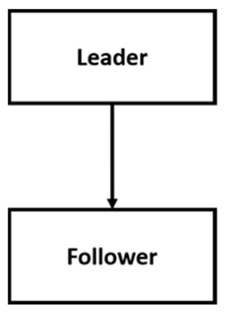
A special case of a multi-level programming problem(MLPP) with a two levels structure is the bi-level programming problem (BLPP) [44]. The general form of the BLPP structure is shown in Figure 3.
Assume that upper-level decision-makers are given control over X, and lower-level decision-makers are given control over Y. Thus, we have   x X R P ,   y Y R q , and F ,   f : R P × R q R 1 . The general BLPP can be formulated as follows:
Min x ϵ X F ( x , y )   ( Leader )
s . t .       G ( x , y ) 0
where y, for each x fixed, solves the problems Equations (3) and (4).
Min y ϵ Y f ( x , y )   ( Follower )
s . t .       g ( x , y ) 0
The leader is the upper-level decision-maker Equation (1), and the follower is the lower-level decision-maker Equation (3). Depending on the demands of the model, x and y may have some additional restrictions, such as integer restrictions or limits on upper and lower bounds.
Based on these, we have the following definitions [45]:
Definition 1.1.
  • The problem constraint region,
S = { ( x ,   y ) X × Y : G ( x , y ) 0 ,   g ( x ,   y ) 0 }
2.
The follower feasible set for each fixed x,
S ( x ) = { y Y : g ( x ,   y ) 0 }
3.
The follower rational reaction set,
P ( x ) = { y Y : y a r g   m i n [ f ( x , y ) : y S ( x ) ] } .
4.
The problem inducible region (IR),
I R = { ( x , y ) : ( x , y ) S , y P ( x ) } .
5.
The problem optimal solution set,
O S = { ( x , y ) : ( x , y ) a r g m i n [ F ( x , y ) : ( x , y ) I R ] }
Definition 1.2.
This section may be divided into subheadings. It should provide a concise and precise description of the experimental results, their interpretation, as well as the experimental conclusions that can be drawn.
Definition 1.3.
For ( x , y ) I R ,   i f   ( x * , y * ) I R ,   F ( x * , y * ) F ( x , y ) , then   ( x * , y * )   is an optimal solution of problem.

2.5.2. Multi-Level Programming Problem

In many applications, the problem of decentralized decision-making within a hierarchical system tends to include more than two levels, which are known as multi-level programming problems (MLPP). The general form of MLPP—tri-level structure is shown in Figure 4.
For   x X R P ,   y Y R q ,   z Z R r , The general tri-level decision problem presented by Faísca [41] is defined as follows:
Min x ϵ X f 1 ( x , y , z )   ( Leader )
s . t . g 1 ( x , y , z ) 0
where (y, z), for each x fixed, solves the problems Equations (12)–(15)
Min y ϵ Y f 2 ( x , y , z )   ( Middle - level   follower )
s . t . g 2 ( x , y , z ) 0
where z, for each (x, y) fixed, solves the problems Equations (14) and (15)
Min z ϵ Z f 3 ( x , y , z )   ( Bottom - level   follower )
s . t .   g 3 ( x , y , z ) 0
where x, y, z are the decision variables of the leader, the middle-level follower, and the bottom-level follower, respectively;   f 1 , f 2 , f 3 : R P × R q × R r R     are the objective functions of the three decision entities, respectively;   g i : R p × R q × R r R k i ,   i = 1 , 2 , 3     are the constraint conditions of the three decision entities respectively.
Based on these, we have the following definitions [46]:
Definition 2.1.
6.
The problem constraint region,
S = { ( x ,   y , z ) X × Y × Z : g i ( x , y , z ) 0 ,   i = 1 , 2 , 3 }
7.
The middle-level follower feasible set for each fixed x,
S ( x ) = { ( y , z ) Y × Z : z g 2 ( x , y , z ) 0 , g 3 ( x , y , z ) 0 }
8.
The bottom-level follower feasible set for each fixed (x, y),
S ( x , y ) = { z Z : g 3 ( x , y , z ) 0 }
9.
The bottom-level follower rational reaction set,
P ( x , y ) = { z Z : z a r g m i n [ f 3 ( x , y , z ) : z S ( x , y ) ] }
10.
The middle-level follower rational reaction set,
P ( x ) = { y , z Y × Z : ( y , z ) a r g m i n [ f 2 ( x , y , z ) : ( y , z ) S ( x ) , z P ( x , y ) ] }
11.
The problem inducible region,
I R = { ( x , y , z ) : ( x , y , z ) S , ( y , z ) P ( x ) }
12.
The problem optimal solution set,
O S = { ( x , y , z ) : ( x , y , z ) a r g m i n [ f 1 ( x , y , z ) : ( x , y , z ) I R ] }
To develop an efficient algorithm to solve a 3 levels decision problem, it is necessary to explore the geometry of the solution space and the associated theoretical properties. The following assumptions are usually made to ensure that the problem is well formulated in terms of the existence of a solution.
Assumption 2.1.
f 1 , f 2 , f 3 , g 1 , g 2 , g 3   are continuous functions, whereas    f 2 , f 3 , g 1 , g 2 , g 3   are continuously differentiable.
Assumption 2.2.
f 3   is strictly convex in z for   z S ( x , y )   where S ( x , y ) is a compact convex set, while f 2 is strictly convex in   ( y , z )   for   ( y , z ) S ( x )   where   S ( x )   is a compact convex set.
Assumption 2.3.
f 1 is continuous convex in x , y , and z .
Under Assumptions 2.1 and 2.2, the rational reaction sets of the bottom-level follower and the middle-level follower   P ( x , y )   and   P ( x )   are point-to-point maps and closed, which implies that   I R   is compact. Thus, under Assumption 2.3, solving the tri-level decision problem is equivalent to optimizing the leader’s continuous function   f 1   over the compact set   I R . It is well known that the solution to such a problem is guaranteed to exist.
It is noticeable that if the bottom-level follower’s problem is a convex parametric programming problem that satisfies the Karush–Kuhn–Tucker Conditions (KKT) for each fixed   ( x , y )   [45,47], the bottom-level follower’s problem is equivalent to the following KKT Equations (23)–(26):
𝛻 z L ( x , y , z , u ) = 𝛻 z f 3 ( x , y , z ) + u 𝛻 z g 3 ( x , y , z ) ,
u g 3 ( x , y , z ) = 0 ,
g 3 ( x , y , z ) 0 ,
u 0
where   𝛻 z f 3 ( x , y , z ) + u 𝛻 z g 3 ( x , y , z )   is the Lagrangian function of the bottom-level follower,   𝛻 z L ( x , y , z , u )   denotes the gradient of the function, for z and u is the vector of Lagrangian multipliers. A necessary and sufficient condition that   ( y , z ) P ( x )   is that the row vector u exists such that   ( x ,   y ,   z ,   u )   satisfies the KKT Equations (23)–(26).
On this basis, by replacing the bottom-level follower problem with the KKT Equations (23)–(26), the tri-level programming problem can be transformed into a bi-level programming problem. The converted equation is shown below:
Min x f 1 ( x , y , z )   ( Leader )   ( 11 )
where (y, z), for each x fixed, solves the problems Equations (22)–(25)
Min y , z , u f 2 ( x , y , z )   ( Follower )   ( 12 )
𝛻 z f 3 ( x , y , z ) + u 𝛻 z g 3 ( x , y , z ) = 0   ( 24 ) ( 26 )
In this research, the proposed MLiSSO algorithm is extended to solve a multi-level supply chain pricing problem to find a solution ( x , y , z ) based on Equations (11), (12) and (27)–(29).

2.6. Improved Simplified Swarm Optimization (iSSO)

In this study, because of the NP-hard nature of the multi-level model, we propose a solution procedure based on a novel, convenient and efficient heuristic algorithm called improved Simplified Swarm Optimization (iSSO) [17], which is based on the Simplified Swarm Optimization (SSO) [48] that can perform a full domain search over a large feasible solution space and enhance the solution quality of the algorithm during the search process.
In 2009, Yeh designed the Simplified Swarm Optimization (SSO) [43] to overcome the shortcomings of PSO proposed by Kennedy and Eberhart [49], which was developed based on human observation of birds foraging behavior and a little weak for discrete problems. The targeting principle was used to update variables quickly, which only uses one random number, two multiplications, and one comparison after c w , c p , and c g are given in SSO. According to the results of Yeh [50,51], SSO is more efficient in converging to high-quality solution spaces in some problems.
The update mechanism of SSO is very simple, efficient and flexible [48,50,51,52,53,54,55,56], and can be presented as a stepwise-function update:
x i j t + 1 = { g j ,           i f ρ [ 0 , 1 ] [ 0 , C g )     p i j ,         i f ρ [ 0 , 1 ] [ C g , C p ) x i j t ,         i f ρ [ 0 , 1 ] [ C p , C w ) x ,         i f ρ [ 0 , 1 ] [ C w , 1 )
All variables need to be updated in traditional SSO (called all-variable update), i = 1 ,   2 ,   ,     N s o l ,   j = 1 ,   2 ,     ,     N v a r ,   t = 0 ,   1 ,   2 ,     ,     N g e n 1 . Let X i t = { x i 1 t , x i 2 t , , x i N v a r t } represent the ith solution in the t generation, and in the formula of Equation (30), x i j t is expressed as the jth variable in X i t ; N v a r represents the number of variables;   c w , c p , and c g are a preset constant; p i j t is the best solution in its evolutionary history; g j is the jth variable of the best solution ever, and x is a random number between the lower bound and the upper bound of the jth variable.
Then to further improve the ability of SSO to solve continuous type problems, Yeh introduced the improved Simplified Swarm Optimization (iSSO) in 2015 [17]. A continuous version of SSO with a new update mechanism is proposed in this work to enhance the ability to solve continuous problems with traditional SSO. To date, iSSO has been successfully applied to many sequential problems, as shown in Yeh [57,58], with experimental results demonstrating its effectiveness in solving sequential problems and its ability to produce high-quality solutions. The update mechanism of iSSO is much simpler than the major soft computing technique-PSO (which must calculate both the velocity and position functions) [18,48,54,55,56].
The update mechanism of iSSO can be presented as follows:
x i j t + 1 = { x ij t + r ij [ 0.5 , 0.5 ] t · u j   i f   x ij t = g i   or   ρ ij [ 0 , 1 ] t [ 0 , C r = c r ) g j + r ij [ 0.5 , 0.5 ] t · u j     i f   x ij t g i   and   ρ ij [ 0 , 1 ] t [ C r , C g = c r + c g ) x ij t + r ij [ 0.5 , 0.5 ] t · ( x ij t g j )     i f   x ij t g i   and   ρ ij [ 0 , 1 ] t [ C g , 1 = c r + c g + c w )
u j = x j m i n x j m a x 2 · N v a r
As defined in Equation (36), C r = c r , C g = c r + c g . In addition, in Equation (32), u j is calculated with the variable’s lower-bound x j m i n , the upper-bound x j m a x , and the numbers of variables. For each update, a random number ρ i j t that is uniformly distributed between [0, 1] is randomly generated first, and r i j t is a random number that is uniformly distributed between [−0.5, 0.5]. To compare ρ i j t with the three constants C r , C g , and C w , if 0 < ρ i j t < C r , the variable is updated according to the first term of Equation (31); if t, the variable is updated according to the second term of Equation (31) to find the adjacent values of g. If C r < ρ i j t < C g , the variable will be updated according to the third term of Equation (36) to find a value between the interval from itself to g j .
If the variable does not meet the upper and lower bound restrictions, the variable will be set to the nearest boundary value. If X i t + 1 does not outperform X i t in the target function, then X i t + 1 = X i t and will not be updated.
So far, only a few papers have studied dual-channel supply chains under capital constraints, which can be regarded as an MLPP. To solve these problems, we apply a continuous-type algorithm iSSO on MLPP to deal with these pricing strategy problems. The detailed algorithmic procedure will be presented and explained in Section 4.

3. Statement

3.1. Model Description

To solve the optimal pricing strategy for the overall supply chain and to further illustrate the hierarchical and interactive relationships among the supply chain decisions, we use a multi-level programming problem to describe the master-slave decision structure of the proposed capital constraint dual-channel supply chain model by Zhen [18]. The Stackelberg game is applied to the model due to the aforementioned level structure of the supply chain system and the sequential relation of decision-making is consistent with the context set. As a result and according to the different financing strategies, the supply chain structure can be divided into two types: bi-level and tri-level planning models to present the decisions made by all members of the supply chain in pursuit of their own optimal goals while considering the optimal responses of each other. This chapter introduces the assumptions, notations, and mathematical models of the problem.

3.2. Assumptions

All assumptions regarding the study are described below.
  • This study constructs a dual-channel supply chain model with three levels of the supply chain (manufacturer → retailer → customer) to profit maximization.
  • The manufacturer’s initial capital is zero and must repay the entire capital liability.
  • The basic principle of profitability is that the price must be designed to meet the conditions of profitability for all parties.
  • In the model, neither the upstream manufacturer nor the downstream manufacturer considers the inventory problem. The upstream manufacturer ships as much product as it makes to the downstream retailer. The downstream manufacturer buys as much as it can and sells it all to the market.

3.3. Notations

According to the article published by Zhen [18], the notation in Table 1 is used in the capital-constrained dual-channel supply chain model.
In general, in each channel, the demand is mainly influenced by its own price; therefore, it is assumed that b > d . In addition, we also assume a > ( b d ) ( P M + P R ) as the demand is not negative.

3.4. The Mathematical Model Description

A dual-channel supply chain with the aim of profit maximization is considered in this article, with a manufacturer to produce a unit product at cost c . The manufacturer has two sales channels in this market. One is the retail channel, where the manufacturer sells the product at wholesale price w to the retailer, which sells it at retail price P R to the consumer, and this channel is also known as the traditional channel. The other channel is the direct sales channel. The manufacturer sells the products directly to the consumers at the selling price P M through a third-party platform, also called the third-party platform channel. The structure of the supply chain model is shown in Figure 5; the solid black line indicates that the products are sold to retailers through wholesale; the dotted black line indicates that the products are sold directly through a third-party online platform, and the platform fee η is paid for the cooperation.
In addition, the demands in this market are variables, defined as manufacturer demand q M and retailer demand q R , respectively. It is assumed that the demand structure of this supply chain is a linear price dependence, which is widely used in the literature [59]. The demand functions are as follows,
q R = λ a b P R + d P M
q M = ( 1 λ ) a b P M + d P R
where b means that a unit of price reduction increases the demand by b, corresponding to marginal and switching customers. A large value of d corresponds to switching customers who are sensitive to differences between the selling price and the retail price. In other words, the degree of differentiation between direct and retail channels decreases as d increases. Thus, d captures the degree of competition between the two channels [60,61].
To find the optimal financing decision and related pricing outcome for this model, we try to maximize the profits for manufacturers, retailers, third-party platforms, and the bank. The objective function and constraints of the model are described in the next part.

3.5. Model Construction

Based on the proposed dual-channel supply chain model proposed in [18] and due to the hierarchical decision relationship of the model, we formulate the supply chain model as an MLPP according to the literature review as follows:
(a)
Retailer
M a x = w R q R R + ( 1 η ) P M R q M R c ( 1 + r R ) ( q M R + q R R )
M a x = ( P R R w R ) q R R + r R c ( q M R + q R R )
(b)
Bank
M a x   f 1 = w B q R B + ( 1 η ) P M B q M B c ( 1 + r B ) ( q M B + q R B )
M a x   f 2 = ( P R B w B ) q R B
M a x   f 3 = r B c ( q M B + q R B )
(c)
3rd Party Platform
M a x   f 1 = w T q R T + ( 1 η ) P M T q M T c ( 1 + r T ) ( q M T + q R T )
M a x   f 2 = ( P R T w T ) q R T
M a x   f 3 = η P M T q M T + r T c ( q M T + q R T ) .
(d)
Constraints of all
s . t .   a > ( b d ) ( P M i + P R i )
w i q R + ( 1 η ) P M i q M i > c ( q R i + q M i ) ( 1 + r i )
P R i w i c ( 1 + r i )
P M i c ( 1 + r i )
P M i w i
Equation (35) means the manufacturer’s maximum profit with retailer finance strategy, and Equation (36) means the retailer’s maximum profit with retailer finance strategy.
Equation (37) means the manufacturer’s maximum profit with bank finance strategy, Equation (43) means the retailer’s maximum profit with bank finance strategy, and Equation (38) means the bank’s maximum profit with bank finance strategy.
Equation (39) means the manufacturer’s maximum profit with a third-party platform finance strategy, Equation (40) means the retailer’s maximum profit with a third-party platform finance strategy, and Equation (41) means the third-party platform’s maximum profit with a third-party platform finance strategy.
These three problems all share the same constraints for each layer of Equations (43)– (47). For Equation (43) means demand should not be negative. To fulfill Equation (44), manufacturers must set a selling price that ensures their revenue is greater than its cost. For Equations (45) and (46), we assume that channel prices must exceed marginal costs. For Equation (47), the retailer cannot purchase from the direct channel, so the selling price of the direct channel must not be lower than the wholesale price.

4. Methodology

4.1. Multi-Level Improved Simplified Swarm Optimization (MLiSSO)

In this study, we propose an MLiSSO approach to apply iSSO to MLPP, including the following functional concepts, which are described in detail in the subsequent subsections.
The basic idea of MLPP can be explained as follows, for a strategy given by the leader, followers are assumed to react rationally. The resulting decisions of the leader and the followers can be considered as the “outcome” of the problem. If the leader chooses a different strategy, the outcome will change accordingly. The inducible region is then defined as the set of these outcomes for all the leader’s strategies. Thus, the best outcomes that the leader can induce are the best results in the inducible region.
Therefore, in this paper, based on the main constraints of MLPP solving, we use the following methods to ensure the implementation of the above ideas and to avoid the problem of the solving process falling into the best solution of the region, as well as to ensure that it presents the characteristics of the MLPP model and the generation of feasible solutions.

4.1.1. Improved Simplified Swarm Optimization (iSSO)

For the update mechanism iSSO we used in this paper, which is mentioned in the literature review [17], to maintain the diversity of the solution, we add the condition of partial best p i j back into the formula, set the random range for turbulence to [ 0.001 ,   0.001 ] , and make the value of u j decrease as the number of generations increases. Equations (48) and (49) are the core formulas when iSSO evolves. Thus, there are four evolution scenarios for x i j t + 1 : oscillating near g j , oscillating near P i j , oscillating near the original value, or evolving to the point between the original value and g j . The evolution decision is determined by ρ i j t .
The modified formula is as follows:
x i j t + 1 = { g j + ρ [ 0.001 , 0.001 ] · u j if   x i j t g j   and   ρ [ 0 , 1 ] [ 0 , C g ) p i j + ρ [ 0.001 , 0.001 ] · u j if   x i j t g j   and   ρ [ 0 , 1 ] [ C g , C p ) x i j t + ρ [ 0.001 , 0.001 ] · u j if x i j t = g j   or   ρ [ 0 , 1 ] [ C p , C w ) x i j t + ρ [ 0.001 , 0.001 ] · ( x i j t g j ) if   x i j t g j   and   ρ [ 0 , 1 ] [ C w , 1 ]
u j = x j m i n x j m a x 2 · N g e n N v a r
If any variable violates the boundary condition, it is set to the nearest boundary after using Equation (53). The steps are shown in detail in the following Section 4.1.7

4.1.2. Fixed-Variables Local Search

Based on the hierarchical properties of the MLP problem, we introduce a local search method with fixed variables in MLiSSO. In traditional SSO, the initial solution is generated randomly between the lower and upper bounds at the same time. When SSO updates the position, the solutions of all dimensions are changed simultaneously. In this study, only the solution of the decision variable of that level is changed when it is updated and then the local search is executed. The solutions of the remaining levels keep the original results. The calculation process is explained in detail in the following Section 4.1.7.

4.1.3. Fitness Function

For the BLPP structure mentioned in the literature review Equations (1)–(4), the upper and lower levels of the programming problem are both standard constraints optimization problems that do not consider the information interaction between the leader and the follower. We treat the lower-level programming problem as a separate constraint optimization problem without losing the general approach to describe constraint processing techniques. In this case, the fitness of all particle updates can be calculated according to Equation (50); the fitness of the best solution is calculated and evaluated according to Equation (51):
f i t n e s s ( x , y ) = { f ( x , y ) ,                   i f y S ( x )               F ( x , y ) ,                   i f y S ( x ) / S        
where S ( x ) denotes the lower-level programming problem feasible set and S denotes the constraint region. The fitness value is calculated differently according to the updated level. For the upper-level update, we generate the value of F ( x , y ) , and for the lower-level update, we generate the value of f ( x , y ) , due to the level having different objective functions to obtain their optimal value.
f i t n e s s ( x , y ) = F ( x , y ) ,     i f y S ( x ) / S
The MLiSSO targets the leader’s priority first. Therefore we use the higher-level objective functions for the best solution evaluation to ensure that we always put the leader’s interest first in a multilevel programming situation. The calculation of all processes is explained in detail in the following Section 4.1.7.

4.1.4. Constraint Handling

In this study, to make the solutions obtained by MLiSSO conform to the problem constraints, we propose a simple but effective constraint method that ensures that the solutions generated during its operation are all conforming to the various constraints of the problem.
We use conditional constraints to enforce domain integrity by restricting the solutions generated after iterative updates to acceptable values that match the domain restrictions. A Boolean operator is used to establish the constraints, and when a solution is generated, it is determined whether it satisfies the constraints, and the result is returned. If the result meets the constraint, it is accepted as True and proceeds to the next step of the process; if it violates any of the constraints, it is rejected as False and generates a random set of solutions that meet the variable limitations (upper bound and lower bound), then redo the Boolean evaluation, repeating this step until it is accepted.

4.1.5. Stopping Criteria

There are two major stopping criteria used:
  • The generation number.
  • The maximum iteration.
It will terminate the MLiSSO algorithm after it has reached the maximum number of iterations or generations.

4.1.6. Level Conversion

Based on the literature review that we referred to above, the problem of tri-level supply chains required to be solved in this study can be transformed into a bi-level programming problem through the use of Kuhn–Tucker conditions Equations (23)–(26) to convert the problem to the term as Equations (27–(29) and Equations (11)–(12). The transformed supply chain equation is shown in Equations (52)–(57), Equations (11), Equations (13) and Equation (13) below:
Max x F = w i q R i + ( 1 η ) P M i q M i c ( 1 + r i ) ( q M i + q R i )   ( 11 )
where (y, z, u), for each x fixed, solves the problems Equations (59)–(66)
Max y , z , u f = ( P R i w i ) q R i   ( 13 )
0.4 ( q M i + q R i ) u 1 [ 0.4 ( q M i + q R i ) ] 0.4 u 2 0.4 u 3 = 0
u 1 [ w i q R i ( 1 η ) P M i q M i + 0.4 ( 1 + r i ) ( q M i + q R i ) ] = 0 ,
u 2 [ w i + 0.4 ( 1 + r i ) ] = 0 ,
u 3 [ P M i + 0.4 ( 1 + r i ) ] = 0 ,   ( 15 ) ,   ( 26 )

4.1.7. Steps of MLiSSO for Solving MLPP

The steps of MLiSSO to solve MLPP are described in this section. With one main program and two subprograms are included, which are based on iSSO algorithms. The details are explained as follows.
Main Program: The best solution to solving
STEP 1-1 Maximum   iteration   T m a x .
STEP 1-2 Set   T m a x T = 0 .
STEP 1-3 Call   Subprogram 1   and   generate   the   initial   solution   ( X i T , Y i T ) .
STEP 1-4 Evaluate   F ( X i T , Y i T ) and   let   ( X * , Y * ) = ( X i T , Y i T ) .
STEP 1-5 Fixed   Y i T to the upper-level programming model.
STEP 1-6 Let   T = T + 1 .
STEP 1-7 Call   Subprogram 2   to   generate   X i T .
STEP 1-8 Fixed   the   solution   X i T .
STEP 1-9 Call   Subprogram 2   to   generate   Y i T .
STEP 1-10 Fixed   ( X i T , Y i T )   into   the   objective   function   to   evaluate   the   value   of   the   objective   function .   If   F ( X i T , Y i T ) > F ( X * , Y * ) ,   ( X i T , Y i T )   it   is   recorded   as   ( X * , Y * ) .
STEP 1-11 Stopping   criterion :   if   T T m a x go to STEP 1-12; otherwise, go to STEP 1-6.
STEP 1-12 Output   ( X * , Y * ) and   the   objective   function   value   of   the   upper - level   F ( X * , Y * )   and   the   lower - level   f ( X * , Y * ) .
Subprogram 1: Solution initialization
STEP 2-1Initiate N s o l , N g e n , N v a r , C g , C p , and C w , and the upper and lower bounds of each variable.
STEP 2-2Set N g e n   t = 0 and i = 1 , where i = 1 , 2 , ,   N s o l .
STEP 2-3Generate ( X i T t , Y i T t ) . Let P f i T = ( X i T t , Y i T t ) , and calculate f ( P f i T ) = f ( X i T t , Y i T t ) for i = 1 , 2 , ,   N s o l . And find Gbest such that f ( P f G T ) is the best, and then let t = 1 and i = 1 .
STEP 2-4Generate ρ and calculate u j .
STEP 2-5Generate r to update the X i T t and Y i T t , and calculate f ( X i T t , Y i T t ) .
STEP 2-6 If   f ( X i T t , Y i T t ) > f ( P f i T ) , then P f i T = ( X i T t , Y i T t ) ; Otherwise, go to STEP 2-8.
STEP 2-7If f ( P f i T ) > f ( P f G T ) , then P f G T = P f i T .
STEP 2-8If i N s o l then i = i + 1 and return to STEP 2-4.
STEP 2-9If t < N g e n then   t = t + 1  and  i = 1 , and return to STEP 2-4. Otherwise, go to STEP 2-10.
STEP 2-10Output P f G T = ( X i T , Y i T ) .
Subprogram 2: Level updating solving
STEP 3-1 Initiate   N s o l for both levels, N g e n l (if updating with upper-level l = 1 ; otherwise, l = 2 ) ,   N v a r ,   C g , C p ,   and   C w , and the upper and lower bounds of each variable.
STEP 3-2 Set   N g e n l   t = 0   and   i = 1 ,   where   i = 1 , 2 , ,   N s o l .
STEP 3-3 Generate   X i T t   or   Y i T t .   Let   P F i T = ( X i T t , Y i T ) ,   P f i T = ( X i T , Y i T t ) ,   and   calculate   F ( P F i T ) = F ( X i T t , Y i T ) ,     f ( P f i T ) = f ( X i T , Y i T t )   for   i = 1 , 2 , ,   N s o l .   And   find   Gbest   such   that   F ( P F G T )   or   f ( P f G T )   is   the   best ,   and   then   let   t = 1   and   i = 1 .
STEP 3-4 Generate   ρ   and   calculate   u j .
STEP 3-5 Generate   r   to   update   X i T t   and   Y i T t   and   calculate   F ( X i T t )   and   f ( Y i T t ) .
STEP 3-6 For   upper - level   update ,   If   F ( X i T t , Y i T )   >   F ( P F i T ) ,   then   P F i T = ( X i T t , Y i T ) ;   for   lower - level   update ,   if   f ( X i T , Y i T t )   >   f ( P f i T ) ,   then   P f i T = ( X i T , Y i T t ) ; Otherwise, go to STEP 3-8.
STEP 3-7 For   upper - level   update ,   if   F ( P F i T )   >   F ( P F G T ) ,   then   P F G T = P F i T ;   for   lower - level   update ,   if   f ( P f i T )   >   f ( P f G T ) ,   then   P f G T = P f i T .
STEP 3-8 If   i N s o l ,   then   i = i + 1 and return to STEP 3-4.
STEP 3-9 If   t < N g e n l   then   t = t + 1   and   i = 1 , and return to STEP 3-4. Otherwise, stop.
STEP 3-10 Output   P F G T   o r   P f G T .

5. Data Analysis and Results

Section 5 is divided into two subsections. The first subsection presents a comparative analysis of the differences between the performance of the proposed algorithms in this thesis and other algorithms based on other papers. In the second section, the proposed methodology is applied to the actual supply chain problem, and the pricing decision results are analyzed.

5.1. Numerical Experiments

To test and demonstrate the above concept, three different types of numerical examples taken from the literature are presented. For comparison, in this study, 20 runs were performed (for problem 1 is 30 runs according to the compared algorithm results) for each problem. The standard deviation was calculated with the formula listed below in Table 2, where the standard deviation is based on the upper-level objective function.

5.1.1. Experimental Datasets

In this study, we used four questions used in previous literature as the datasets for the validation tests; the functions are as shown in Table 3, Table 4 and Table 5. The dataset parameters were set according to the parameters used in the reference source data.

5.1.2. Experiments with Orthogonal Arrays

The experimental design of the MLiSSO setup was carried out using a two-factor, two-level full factorial design with four experimental combinations. Including the parameter pbest, and the modification of the u value according to the above mentioned in Section 4.
Each of the above-mentioned three experimental datasets was used to perform independent configuration experiments to identify the most suitable configurations, and Table 6 and Table 7 show the configuration combinations.
The following experiments were compiled using python 3.8 with the same basic parameters, C g = 0.2 ,   C p = 0.3 ,   C w = 0.5 , number of particles = 20, number of generations = 200 (for subprogram), and iterations= 500 (for main program).
Each experiment was run 20 times, and the results were evaluated and analyzed by using the leader’s target function value results. Assuming that the samples conformed to the norm, an analysis of variance (ANOVA) with α = 0.05 was conducted to select the most suitable configuration.
Dataset: Problem 1
Table 8 shows that the p-values of factors A is smaller than α = 0.05, so the factors did cause significant differences, and the p-value of factor B were greater than α = 0.05, so the factors did not cause significant differences. However, factor B was more likely to cause differences than factor A, as shown in Table 9, which shows the mean value of 20 experiments for each of the four groups of experiments
From Figure 6, it can be concluded that the A factor has better performance at level 2 than level 1, and the B factors have better performance at level 1 than at level 2. But, according to the interaction plot, as shown in Figure 7, it indicates the existence of interaction, and we cannot tell if the configuration settings will have better performance by all set to level 2.
Dataset: Problem 2
Table 10 shows that the p-values of both factors A and B are smaller than α = 0.05, so the factors did cause significant differences; furthermore, the factor B was more likely to cause differences than the factor A, as shown in Table 11, which is the mean values of 20 experiments for each of the four groups of experiments.
From Figure 8, it can be concluded that both A and B factors have better performance at level 2 than at level 1, which also has a significant difference in the performance. However, the interaction plot, as shown in Figure 9, it indicates the existence of interaction, and we cannot tell if they could have better performance by all set to level 2.
Dataset: Problem 3
Table 12 shows that the p-values of factors A and B were greater than α = 0.05, so the factors did not cause significant differences; however, factor A was more likely to cause differences than factor B, as shown in Table 13, which is the mean values of 20 experiments for each of the four groups of experiments.
From Figure 10, it can be concluded that the A factor has better performance at level 2 than level 1, and the B factors have better performance at level 1 than at level 2. However, the interaction plot, as shown in Figure 11, it indicates the existence of interaction, and we cannot tell if the configuration settings will have better performance by all set to level 2.
Result Summary
The results of the experiments for the above four configurations are listed and discussed. As shown in Table 14, Table 15 and Table 16, it can be concluded that when both factors A and B are set to level 2 (setting 4), the results obtained for this configuration are superior to those in the other configurations in all three experiments. This setting 4 is also the MLiSSO configuration proposed in this study. Therefore, based on this result, the proposed MLiSSO will be used for other experiments and analyses in the following.

5.1.3. Comparison Experiment Results

In this study, we solved three sets of MLPP problems with different levels of complexity by using MLiSSO and compared the results with those of algorithms proposed in other related literature.
Dataset: Problem 1
We constructed a linear BLPP with multiple leaders and followers from [62] as a numerical example to analyze more complex problems; the functions of problem 1 are listed in Table 3.
In this problem, the parameters setting of two different algorithms, GA [64] and PSO, are given in [11], then we used the trial-and-error method for the setting of MLiSSO, and summarized in Table 17. In addition, as mentioned above, the number of iterations of MLiSSO is indicated by generation(update) and iteration(main), while other algorithms used for comparison are indicated by iteration if not specified. The best optimal solution, mean, and standard deviation values of the solutions for 30 runs are presented in Table 18 and Table 19. Figure 12 shows the convergence of the optimal solution target function value   F ( X ,   Y ) in MLiSSO.
Table 18 and Table 19 indicate that MLiSSO has the smallest standard deviation according to the objective value priority of the leader in the case of linear bi-level decision-making with multiple leaders and multiple followers. It returns better results than the GA, just after the results of PSO with a difference of 0.0157 in terms of the best result. In addition, the average solutions of MLiSSO return significantly better than the solutions of other algorithms in the average result, and the standard deviation of the MLiSSO method is lower than that of other algorithms. This indicates that MLiSSO has higher stability and provides better solution quality for solving complex problems.
In the study of Kuo & Huang [11], for the initial solution, they adopt the float coding method to generate the random numbers for the upper-level variables and program for variables in the lower level. Then, update the velocity and position for every particle at once. To compare with the results, we use the same structure and iteration = 150 to generate the results, which are listed in the right column (as literature) in Table 18 and Table 19.
The results show that if we only use the proposed modified iSSO with the same kind of structure, the best result and the average result are both superior to the other two methods, and the average result is just after the original MLiSSO. However, the purpose of MLiSSO is for general use on other types of MLPP when this method is only used on linear programming problems mentioned in the literature, so we use the following non-linear problems to emphasize the commonality of MLiSSO.
Dataset: Problem 2
For the example of nonlinear BLPP, which was constructed from [63], the functions of problem 2 are listed in Table 4. In this problem, the two different algorithms, evolutionary algorithm (EA) and PSO-CST are given in [65,66], and the setup of the parameters is listed in Table 20. In addition, as mentioned above, the number of iterations of MLiSSO is indicated by generation (update) and iteration (main), while other algorithms used for comparison are indicated by iteration if not specified. The best optimal solution, mean, and standard deviation values of the solutions for 20 runs are shown in Table 21, and because the average results are not given in the literature [65,66], we only list the result of MLiSSO. Figure 13 shows the convergence of the optimal solution target function value F ( X ,   Y ) in MLiSSO.
In the case of this problem, we conclude from Table 21 that MLiSSO outperforms the other algorithms in terms of the objective priority of the leaders and the standard deviation of the solutions obtained is only 0.1396, which means that its solutions remain fairly stable. Thus, MLiSSO shows better performance than these two algorithms for the nonlinear BLPP. This result also implies that the proposed MLiSSO is suitable for solving nonlinear multi-player BLPP.
Dataset: Problem 3
We constructed a nonlinear BLPP with a single leader and follower from [6] as a numerical example to analyze more complex problems(cube); the functions of problem 1 are listed in Table 5.
In this problem, the two different algorithms, HPSOBLP and IBPSO, are given in [6,67], with parameter settings summarized in Table 22. In addition, as mentioned above, the number of iterations of MLiSSO is indicated by generation (update) and iteration (main), while other algorithms used for comparison are indicated by iteration if not specified. The best optimal solution, mean, and standard deviation values of the solutions for 20 runs are presented in Table 23 and Table 24. Figure 14 shows the convergence of the optimal solution target function value F(X,Y) in MLiSSO
Table 23 and Table 24 indicate that MLiSSO outperforms the other algorithms in terms of the objective priority of the leaders, which means that MLiSSO has a better performance than these two algorithms. In addition, also the average results show that the solution can be obtained with better quality in several independent experiments.

5.2. Model Evaluation

Based on the aforementioned experimental results, it can be stated that MLiSSO can be used to solve the MLPP with a higher stability quality of optimal solution results. This section further verifies the practicality of the MLiSSO on supply chain problems by using the supply chain model with three different financing strategies Equations (40)–(47) and constraints of them Equations (48)–(52). The parameters setup of the supply chain model is, according to Zhen [18], listed in Table 25, and the parameter setup of MLiSSO is listed in Table 26. The corresponding solutions of the three financing strategy models are shown in Table 27 and Table 28. Figure 15 and Figure 16 show the convergence of the optimal solution target function value F ( X , Y ) in MLiSSO
As shown in Table 27 (1) for the retailer-financed case, the objective value of the leader has converged to f 1 ( x ,   y ,   z ) = 0.03231 , while the objective value of layers 2 have converged to   f 2 ( x ,   y ,   z ) = 0.00756 ; (2) for the bank-financed case, the objective value of the leader has converged to f 1 ( x ,   y ,   z ) = 0.04068 while the objective values for layers 2 and 3 converge to f 2 ( x ,   y ,   z ) = 0.00284 and   f 3 ( x ,   y ,   z ) = 0.00168 ; (3) the third-party platform-financed case, the objective value of the leader has converged to f 1 ( x ,   y ,   z ) = 0.04068 , while the objective values for layers 2 and 3 converge to f 2 ( x ,   y ,   z ) = 0.00284 and f 3 ( x ,   y ,   z ) = 0.01487 . We also list the average and standard deviation of the solutions we obtained in 20 runs in Table 28.
It can be noted that under this group of market conditions of parameters and after conversion calculation, as shown in Table 27, we learn that among all financing options, the financing strategy with third-party platforms and banks has absolutely favorable conditions for manufacturers. Thus, it can be concluded that this approach can be applied to complex and practical decision problems to solve MLPP.

6. Conclusions

First, we review this paper; our proposed method uses hierarchical updates of fixed variables, trivial problem transformations, computation of objective functions, and iSSO algorithms. Although it does not outperform the best current algorithms for the related small-scale problems, it surpasses the performance of other algorithms for large-scale problems. In conclusion, due to the average and standard deviation of the results, it provides a relatively stable, feasible, and effective solution to the MLPP problem and can be applied to the relevant decision-making process. On the other hand, this paper uses a fixed-variable approach to search, which can express the concept of hierarchical decision-making more effectively and can be implemented on higher-level MLPs that introduce multiple leaders and multiple followers to achieve a more realistic large-scale goal problem. It is also easier to extend to solve a complex problem. If further exploration and experimentation can be done, it may further enhance the ability of this solution to solve problems.
In recent years, many researchers have been studying hybrid algorithms for solving MLPP problems, and as the complexity of the problems increases, mathematical research will become more practical. Therefore, it is expected that more ways and improvements will be developed to solve related problems to meet the industry’s current needs.
With the results of this study, the necessity of investigating many of these issues is highlighted, especially to improve the methodology of MLPP. Among the many topics to be explored in future research, there are several major extensions that we intend to focus on.
(1)
Hybridization of other heuristic mechanisms to improve MLiSSO solving
(2)
Consider the dynamical mechanism for adjusting the upper and lower terms in terms of the turbulence of the update mechanism to improve the generated solutions towards the desired optimal solution to improve the efficiency and quality of the solutions.

Author Contributions

Conceptualization, Z.L. and W.-C.Y.; methodology, Z.L., Y.-C.Y. and W.-C.Y.; writing—original draft preparation, Z.L.; writing—review and editing, Z.L. and S.-Y.T. All authors have read and agreed to the published version of the manuscript.

Funding

This research received no external funding.

Institutional Review Board Statement

Not applicable.

Informed Consent Statement

Not applicable.

Data Availability Statement

All data included in the main text.

Conflicts of Interest

The authors declare no conflict of interest.

References

  1. Matsui, K. When should a manufacturer set its direct price and wholesale price in dual-channel supply chains? Eur. J. Oper. Res. 2017, 258, 501–511. [Google Scholar] [CrossRef]
  2. Ma, J.; Wang, H. Complexity analysis of dynamic noncooperative game models for closed-loop supply chain with product recovery. Appl. Math. Model. 2014, 38, 5562–5572. [Google Scholar] [CrossRef]
  3. Von Stackelberg, H. Marktform Und Gleichgewicht; Springer: Berlin/Heidelberg, Germany, 1934. [Google Scholar]
  4. Grand, S.; Von Krogh, G.; Leonard, D.; Swap, W. Resource allocation beyond firm boundaries: A multi-level model for open source innovation. Long Range Plan. 2004, 37, 591–610. [Google Scholar] [CrossRef]
  5. Dotoli, M.; Fanti, M.P.; Meloni, C.; Zhou, M.C. A multi-level approach for network design of integrated supply chains. Int. J. Prod. Res. 2005, 43, 4267–4287. [Google Scholar] [CrossRef]
  6. Ma, W.; Wang, M.; Zhu, X. Improved particle swarm optimization based approach for bilevel programming problem-an application on supply chain model. Int. J. Mach. Learn. Cybern. 2014, 5, 281–292. [Google Scholar] [CrossRef]
  7. Ben-Ayed, O.; Blair, C.E. Computational difficulties of bilevel linear programming. Oper. Res. 1990, 38, 556–560. [Google Scholar] [CrossRef]
  8. Bard, J.F. Some properties of the bilevel programming problem. J. Optim. Theory Appl. 1991, 68, 371–378. [Google Scholar] [CrossRef]
  9. Segall, R. Using branch-and-bound to solve bi-level geometric programming problems: A new optimization model. Appl. Math. Model. 1990, 14, 271–274. [Google Scholar] [CrossRef]
  10. Kasemset, C.; Kachitvichyanukul, V. A PSO-based procedure for a bi-level multi-objective TOC-based job-shop scheduling problem. Int. J. Oper. Res. 2012, 14, 50–69. [Google Scholar] [CrossRef]
  11. Kuo, R.; Huang, C. Application of particle swarm optimization algorithm for solving bi-level linear programming problem. Comput. Math. Appl. 2009, 58, 678–685. [Google Scholar] [CrossRef]
  12. Liu, B. Stackelberg-Nash equilibrium for multilevel programming with multiple followers using genetic algorithms. Comput. Math. Appl. 1998, 36, 79–89. [Google Scholar] [CrossRef]
  13. Kliestik, T.; Zvarikova, K.; Lăzăroiu, G. Data-driven machine learning and neural network algorithms in the retailing environment: Consumer engagement, experience, and purchase behaviors. Econ. Manag. Financ. Mark. 2022, 17, 57–69. [Google Scholar]
  14. Hopkins, E. Machine Learning Tools, Algorithms, and Techniques. J. Self-Gov. Manag. Econ. 2022, 10, 43–55. [Google Scholar]
  15. Nica, E.; Sabie, O.M.; Mascu, S.; Luţan, A.G. Artificial Intelligence Decision-Making in Shopping Patterns: Consumer Values, Cognition, and Attitudes. Econ. Manag. Financ. Mark. 2022, 17, 31–43. [Google Scholar]
  16. Kliestik, T.; Kovalova, E.; Lăzăroiu, G. Cognitive decision-making algorithms in data-driven retail intelligence: Consumer sentiments, choices, and shopping behaviors. J. Self-Gov. Manag. Econ. 2022, 10, 30–42. [Google Scholar]
  17. Yeh, W.-C. An improved simplified swarm optimization. Knowledge-Based Syst. 2015, 82, 60–69. [Google Scholar] [CrossRef]
  18. Zhen, X.; Shi, D.; Li, Y.; Zhang, C. Manufacturer’s financing strategy in a dual-channel supply chain: Third-party platform, bank, and retailer credit financing. Transp. Res. Part E: Logist. Transp. Rev. 2020, 133, 101820. [Google Scholar] [CrossRef]
  19. Tsay, A.A.; Agrawal, N. Channel Conflict and Coordination in the E-Commerce Age. Prod. Oper. Manag. 2009, 13, 93–110. [Google Scholar] [CrossRef]
  20. Cai, G.G. Channel selection and coordination in dual-channel supply chains. J. Retail. 2010, 86, 22–36. [Google Scholar] [CrossRef]
  21. Yan, R.; Pei, Z. Information asymmetry, pricing strategy and firm’s performance in the retailer-multi-channel manufacturer supply chain. J. Bus. Res. 2011, 64, 377–384. [Google Scholar] [CrossRef]
  22. Chiang, W.-Y.K.; Chhajed, D.; Hess, J.D. Direct Marketing, Indirect Profits: A Strategic Analysis of Dual-Channel Supply-Chain Design. Manag. Sci. 2003, 49, 1–20. [Google Scholar] [CrossRef]
  23. Bernstein, F.; Song, J.-S.; Zheng, X. Free riding in a multi-channel supply chain. Nav. Res. Logist. (NRL) 2009, 56, 745–765. [Google Scholar] [CrossRef]
  24. Ryan, J.; Sun, D.; Zhao, X. Coordinating a Supply Chain with a Manufacturer-Owned Online Channel: A Dual Channel Model Under Price Competition. IEEE Trans. Eng. Manag. 2012, 60, 247–259. [Google Scholar] [CrossRef]
  25. Saha, S. Channel characteristics and coordination in three-echelon dual-channel supply chain. Int. J. Syst. Sci. 2014, 47, 740–754. [Google Scholar] [CrossRef]
  26. Huang, W.; Swaminathan, J.M. Introduction of a second channel: Implications for pricing and profits. Eur. J. Oper. Res. 2009, 194, 258–279. [Google Scholar] [CrossRef]
  27. Tang, C.S.; Yang, S.A.; Wu, J. Sourcing from Suppliers with Financial Constraints and Performance Risk. Manuf. Serv. Oper. Manag. 2018, 20, 70–84. [Google Scholar] [CrossRef]
  28. Lee, C.H.; Rhee, B.-D. Trade credit for supply chain coordination. Eur. J. Oper. Res. 2011, 214, 136–146. [Google Scholar] [CrossRef]
  29. Kouvelis, P.; Zhao, W. Who Should Finance the Supply Chain? Impact of Credit Ratings on Supply Chain Decisions. Manuf. Serv. Oper. Manag. 2018, 20, 19–35. [Google Scholar] [CrossRef]
  30. Kouvelis, P.; Zhao, W. Supply Chain Contract Design Under Financial Constraints and Bankruptcy Costs. Manag. Sci. 2016, 62, 2341–2357. [Google Scholar] [CrossRef]
  31. Caldentey, R.; Haugh, M.B. Supply Contracts with Financial Hedging. Oper. Res. 2009, 57, 47–65. [Google Scholar] [CrossRef]
  32. Aydin, R.; Kwong, C.; Ji, P. Coordination of the closed-loop supply chain for product line design with consideration of remanufactured products. J. Clean. Prod. 2016, 114, 286–298. [Google Scholar] [CrossRef]
  33. Yang, D.; Jiao, J.; Ji, Y.; Du, G.; Helo, P.; Valente, A. Joint optimization for coordinated configuration of product families and supply chains by a leader-follower Stackelberg game. Eur. J. Oper. Res. 2015, 246, 263–280. [Google Scholar] [CrossRef]
  34. Cachon, G.P.; Zipkin, P.H. Competitive and cooperative inventory policies in a two-stage supply chain. Management science 1999, 45, 936–953. [Google Scholar] [CrossRef]
  35. Hennet, J.-C.; Arda, Y. Supply chain coordination: A game-theory approach. Eng. Appl. Artif. Intell. 2008, 21, 399–405. [Google Scholar] [CrossRef]
  36. Tian, Y.; Govindan, K.; Zhu, Q. A system dynamics model based on evolutionary game theory for green supply chain management diffusion among Chinese manufacturers. J. Clean. Prod. 2014, 80, 96–105. [Google Scholar] [CrossRef]
  37. Cachon, G.P.; Netessine, S. Game Theory in Supply Chain Analysis, in Models, Methods, and Applications for Innovative Decision Making; INFORMS: Catonsville, MD, USA, 2006; pp. 200–233. [Google Scholar]
  38. Leng, M.; Parlar, M. Game Theoretic Applications in Supply Chain Management: A Review. INFOR Inf. Syst. Oper. Res. 2005, 43, 187–220. [Google Scholar] [CrossRef]
  39. Stackelberg, H.V.; Von, S.H. The Theory of the Market Economy; Oxford University Press: Oxford, UK, 1952. [Google Scholar]
  40. Zhou, Z.F. Research on Pricing Decision of Multi-Level Remanufacturing Reverse Supply Chain Based on Stackelberg Game. Appl. Mech. Mater. 2012, 220–223, 290–293. [Google Scholar] [CrossRef]
  41. Sadigh, A.N.; Mozafari, M.; Karimi, B. Manufacturer–retailer supply chain coordination: A bi-level programming approach. Adv. Eng. Softw. 2012, 45, 144–152. [Google Scholar] [CrossRef]
  42. Lu, J.; Han, J.; Hu, Y.; Zhang, G. Multilevel decision-making: A survey. Inf. Sci. 2016, 346–347, 463–487. [Google Scholar] [CrossRef]
  43. Luo, H.; Liu, L.; Yang, X. Bi-level programming problem in the supply chain and its solution algorithm. Soft Comput. 2019, 24, 2703–2714. [Google Scholar] [CrossRef]
  44. Colson, B.; Marcotte, P.; Savard, G. Bilevel programming: A survey. 4OR 2005, 3, 87–107. [Google Scholar] [CrossRef]
  45. Bard, J. Practical Bilevel Optimization: Applications and Algorithms, in Series: Nonconvex Optimization and Its Applications; Springer: Berlin/Heidelberg, Germany, 1998. [Google Scholar]
  46. Faísca, N.P.; Saraiva, P.M.; Rustem, B.; Pistikopoulos, E.N. A multi-parametric programming approach for multilevel hierarchical and decentralised optimisation problems. Comput. Manag. Sci. 2007, 6, 377–397. [Google Scholar] [CrossRef]
  47. Dempe, S. Foundations of Bilevel Programming; Springer Science & Business Media: Berlin, Germany, 2002. [Google Scholar]
  48. Yeh, W.-C. A two-stage discrete particle swarm optimization for the problem of multiple multi-level redundancy allocation in series systems. Expert Syst. Appl. 2009, 36, 9192–9200. [Google Scholar] [CrossRef]
  49. Eberhart, R.; Kennedy, J. Particle Swarm Optimization. In Proceedings of the IEEE International Conference on Neural Networks, Perth, Australia, 27 November–1 December 1995. [Google Scholar]
  50. Yeh, W.-C. Orthogonal simplified swarm optimization for the series–parallel redundancy allocation problem with a mix of components. Knowl.-Based Syst. 2014, 64, 1–12. [Google Scholar] [CrossRef]
  51. Yeh, W.-C. Optimization of the Disassembly Sequencing Problem on the Basis of Self-Adaptive Simplified Swarm Optimization. IEEE Trans. Syst. Man, Cybern.-Part A Syst. Hum. 2011, 42, 250–261. [Google Scholar] [CrossRef]
  52. Huang, C.-L.; Jiang, Y.-Z.; Yin, Y.; Yeh, W.-C.; Chung, V.Y.Y.; Lai, C.-M. Multi Objective Scheduling in Cloud Computing Using MOSSO. IEEE Congr. Evol. Comput. 2018, 12, 1–8. [Google Scholar]
  53. Yeh, W.-C. A new exact solution algorithm for a novel generalized redundancy allocation problem. Inf. Sci. 2017, 408, 182–197. [Google Scholar] [CrossRef]
  54. Yeh, W.-C. New parameter-free simplified swarm optimization for artificial neural network training and its application in the prediction of time series. IEEE Trans. Neural Netw. Learn. Syst. 2013, 24, 661–665. [Google Scholar]
  55. Yeh, W.-C. Novel swarm optimization for mining classification rules on thyroid gland data. Inf. Sci. 2012, 197, 65–76. [Google Scholar] [CrossRef]
  56. Yeh, W.-C. Simplified swarm optimization in disassembly sequencing problems with learning effects. Comput. Oper. Res. 2012, 39, 2168–2177. [Google Scholar] [CrossRef]
  57. Yeh, W.-C. A novel boundary swarm optimization method for reliability redundancy allocation problems. Reliab. Eng. Syst. Saf. 2019, 192, 106060. [Google Scholar] [CrossRef]
  58. Lin, P.; Cheng, S.; Yeh, W.; Chen, Z.; Wu, L. Parameters extraction of solar cell models using a modified simplified swarm optimization algorithm. Sol. Energy 2017, 144, 594–603. [Google Scholar] [CrossRef]
  59. Shen, Y.; Willems, S.P.; Dai, Y. Channel Selection and Contracting in the Presence of a Retail Platform. Prod. Oper. Manag. 2018, 28, 1173–1185. [Google Scholar] [CrossRef]
  60. Abhishek, V.; Jerath, K.; Zhang, Z.J. Agency Selling or Reselling? Channel Structures in Electronic Retailing. Manag. Sci. 2016, 62, 2259–2280. [Google Scholar] [CrossRef]
  61. Liu, Y.-H.; Hart, S.M. Characterizing an optimal solution to the linear bilevel programming problem. Eur. J. Oper. Res. 1994, 73, 164–166. [Google Scholar] [CrossRef]
  62. Bard, J.F.; Falk, J.E. An explicit solution to the multi-level programming problem. Comput. Oper. Res. 1982, 9, 77–100. [Google Scholar] [CrossRef]
  63. Amouzegar, M.A.; Cybernetics, P.B. A global optimization method for nonlinear bilevel programming problems. IEEE Trans. Syst. Man Cybern. Part B (Cybern) 1999, 29, 771–777. [Google Scholar] [CrossRef]
  64. Guang-Min, W.; Zhong-Ping, W.; Xian-Jia, W.; Ya-Lin, C. Genetic Algorithms for Solving Linear Bilevel Programming. In Proceedings of the IEEE Sixth International Conference on Parallel and Distributed Computing Applications and Technologies (PDCAT’05), Dalian, China, 5–8 December 2005; pp. 920–924. [Google Scholar]
  65. Wang, Y.; Jiao, Y.-C.; Li, H. An Evolutionary Algorithm for Solving Nonlinear Bilevel Programming Based on a New Constraint-Handling Scheme. IEEE Trans. Syst. Man Cybern. Part C Appl. Rev. 2005, 35, 221–232. [Google Scholar] [CrossRef]
  66. Wan, Z.; Wang, G.; Sun, B. A hybrid intelligent algorithm by combining particle swarm optimization with chaos searching technique for solving nonlinear bilevel programming problems. Swarm Evol. Comput. 2013, 8, 26–32. [Google Scholar] [CrossRef]
  67. Li, X.; Tian, P.; Min, X. A Hierarchical Particle Swarm Optimization for Solving Bilevel Programming Problems. In International Conference on Artificial Intelligence and Soft Computing; Springer: Berlin/Heidelberg, Germany, 2006; pp. 1169–1178. [Google Scholar]
Figure 1. Structure of the dual-channel supply chain.
Technologies 10 00073 g001
Figure 2. Relationship between participants in the Stackelberg game. (a) represents a single leader and follower, (b) represents a single leader and multiple followers, (c) represents multiple leaders and single followers, and (d) represents multiple leaders with multiple followers.
Technologies 10 00073 g002
Figure 3. The general form of BLPP structure.
Technologies 10 00073 g003
Figure 4. The general form of MLPP—tri-level structure.
Technologies 10 00073 g004
Figure 5. Supply chain model.
Technologies 10 00073 g005
Figure 6. Main effects plot of problem 1. A represents factor A in Table 8, B represents factor B in Table 8.
Technologies 10 00073 g006
Figure 7. Interaction plot of problem 1. A represents factor A in Table 8, B represents factor B in Table 8.
Technologies 10 00073 g007
Figure 8. Main effects plot of problem 2. A represents factor A in Table 8, B represents factor B in Table 8.
Technologies 10 00073 g008
Figure 9. Interaction plot of problem 2. A represents factor A in Table 8, B represents factor B in Table 8.
Technologies 10 00073 g009
Figure 10. Main effects plot of problem 3. A represents factor A in Table 8, B represents factor B in Table 8.
Technologies 10 00073 g010
Figure 11. Interaction plot of problem 3. A represents factor A in Table 8, B represents factor B in Table 8.
Technologies 10 00073 g011
Figure 12. Convergence curve when iteration = 500 of problem 1.
Technologies 10 00073 g012
Figure 13. Convergence curve when iteration = 100 of problem 2.
Technologies 10 00073 g013
Figure 14. Convergence curve when iteration = 100 for problem 3.
Technologies 10 00073 g014
Figure 15. Convergence curve of RF.
Technologies 10 00073 g015
Figure 16. Convergence curve of 3PF & BF.
Technologies 10 00073 g016
Table 1. Notations of the dual-channel supply chain model.
TypeSymbolDescription
parameteraThe total potential market size.
λ The   underlying   market   share   of   the   retailer   for   the   manufacturer   is   ( 1 λ ) .   0 λ 1 .
b Demand   sensitivity   to   its   selling / retail   price .   0 < b 1 .
d The   coefficient   of   cross - price   sensitivity .   0 < d 1 .
cProduct production cost.
η Revenue   sharing   of   3 rd   party   platform .   0 < η 1 .
i Finance strategy for:
      i = { B ,   b a n k   f i n a n c e   s t r a t e g y .                                   T ,   3 r d   p l a t f o r m   f i n a n c e   s t r a t e g y . R ,   r e t a i l e r   f i n a n c e   s t r a t e g y .                            
variables w i Wholesale   price ,   for   i = { B T R               N o n e ,   w i 0 .
P R i Retailer s   retail   channel   retail   price ,   with   finance   strategy   for   i = B ,   T   o r   R .   P R i 0 .
P M i Manufacturer s   direct   channel   selling   price   through   3 rd   party   platform ,   with   finance   strategy   for   i = B ,   T   o r   R .   P M i 0 .
q R i Retail   channel   demand ,   with   finance   strategy   for   i = B ,   T   o r   R .
q M i Direct   channel   demand ,   with   finance   strategy   for   i = B ,   T   o r   R .
r i Revenue   sharing   rate ,   with   finance   strategy   for   i = B ,   T   o r   R .   0 < r i 1 .
Table 2. Comparison formula.
FormulaDescription
Standard deviation (SD) i = 1 R ( F M i * F M A * ) 2 R
where   i = 1 , 2 , , R . R = 30 in this paper.
F M i * = The optimal solution for MLiSSO in ith run.
F M A * = The average of R optimal solutions for MLiSSO.
Table 3. Functions for problem 1.
No.Problem Functions
Problem 1 [62] M a x   F = 8 x 1 + 4 x 2 4 y 1 + 40 y 2 + 4 y 3 ,
where   ( y 1 , y 2 , y 3 )   solves,
M a x   f = x 1 2 x 2 y 1 y 2 2 y 3
s.t.
y 1 y 2 y 3 1
2 x 1 + y 1 2 y 2 + 0.5 y 3 1
2 x 2 2 y 1 + y 2 + 0.5 y 3 1
x 1 , x 2 , y 1 , y 2 , y 3 0
Table 4. Functions for problem 2.
No.Problem Functions
Problem 2 [63] M i n   F = x 1 2 3 x 2 2 4 y 1 + y 2 2 ,   where   ( y 1 , y 2 )   solves,
s.t.
x 1 2 + 2 x 2 4
x 1 , x 2 0
M i n   f = 2 x 1 2 + y 1 2 5 y 2
  s.t.
     x 1 2 2 x 1 + x 2 2 2 y 1 + y 2 3
   4 x 2 + 3 y 1 4 y 2 4
   y 1 , y 2 0
Table 5. Functions for problem 3.
No.Problem Functions
Problem 3 [6] M i n   F = x 2 + ( y 10 ) 2 ,   where   y   solves,
s.t.
x + 2 y 6 0 ,
x 0
M i n   f = x 3 2 y 3 + x 2 y x 2
  s.t.
   x + 2 y 3 0 ,
   y 0
Table 6. Factor level table.
Level\Factor Parameter   C p u Value Setting
1WithoutConstant
2Add-inDynamic
Table 7. Full factorial design table.
Setting\Factor Parameter   C p u Value Setting
1WithoutConstant
2WithoutDynamic
3Add-inConstant
4Add-inDynamic
Table 8. ANOVA table of Dataset problem 1.
SourceDFSSMSF-Valuep-Value
A123.40123.40154.530.036
B10.4130.41260.080.778
Error76392.1935.1604
Total79427.4440.000
S = 2.27166R − Sq = 8.25%R − Sq (adj) = 4.63%
Table 9. Response table of Dataset problem 1.
LevelAB
127.527.0
228.026.0
Delta0.51.0
Rank21
Table 10. ANOVA table of Dataset problem 2.
SourceDFSSMSF-Valuep-Value
A10.020500.0205055.130.026
B10.040190.04018710.060.002
Error760.303700.003996
Total790.450290.000000
S = 0.0632139R − Sq = 32.56%R − Sq (adj) = 29.89%
Table 11. Response table of Dataset problem 2.
LevelAB
118.5918.63
218.62518.585
Delta0.0350.045
Rank21
Table 12. ANOVA table of Dataset problem 3.
SourceDFSSMSF-Valuep-Value
A13.13443.13443.240.076
B10.66970.66970.690.408
Error7673.45310.9665
Total7978.85820.0000
S = 0.983102R−Sq = 6.85%R−Sq (adj) = 3.18%
Table 13. Response table of Dataset problem 3.
LevelAB
1−67.5−67.2
2−67.1−67.4
Delta0.40.2
Rank12
Table 14. Results of dataset problem 1.
Setting F a v g F s t d e v F s t d e v F m i n
127.16548632.73279782.732797817.3713556
226.26565563.05033933.050339320.0050241
327.49098921.76622051.766220521.7917118
428.10355100.86570800.865708026.4103750
Table 15. Results of dataset problem 2.
Setting F a v g F s t d e v F s t d e v F m i n
118.60203240.071097518.723180818.4959183
218.58132080.061699118.713613918.4883674
318.56851480.063681118.720290418.4420441
418.67887740.055381318.833493518.6205643
Table 16. Results of dataset problem 3.
Setting F a v g F s t d e v F s t d e v F m i n
167.247013230.97728250968.9393158765.6916659
267.712929411.03198115569.2806171665.54469136
367.134053820.96903105869.1733403465.33748003
467.034126080.95229564867.0341260865.23260349
Table 17. Parameters setup for problem 1.
GA [64]PSO [11]MLiSSO
opulation: 20, Crossover rate: 0.9, Mutation rate: 0.1, Iterations: N/APopulation: 20, Vmax: 10, Inertial weight: 1.2–0.2, Iterations: 150Population: 20, Cg: 0.3, Cp: 0.6, Cw: 0.8, Generations:100/150, Iterations: 500/150
Table 18. Best results of problem 1.
GAPSOMLiSSO
(500)
MLiSSO
(As Literature/150)
x 1 0.0000.00040.00020.0266
x 2 0.8980.89960.89910.0205
y 1 0.0000.00000.00000.7969
y 2 0.5990.59950.59930.7944
y 3 0.3990.39930.39860.1503
F29.148029.178829.663129.4853
f −3.193−3.1977−3.1948−1.9594
Runtime(s)N/AN/A3532
Table 19. Average results & SD of problem 1.
GAPSOMLiSSO
(500)
MLiSSO
(As Literature/150)
x 1 0.157050.021920.000780.01579
x 2 0.864950.866930.896070.18669
y 1 0.000000.00000 0.000000.41225
y 2 0.471920.563350.597010.66371
y 3 0.515920.341080.393510.19149
F21.5294824.8125629.0449426.53842
f −3.39072−3.1977−3.17696−1.84811
F stdev3.144321.553740.106892.23245
Runtime(s)N/AN/A4535
Table 20. Parameters setup for problem 2.
EA [65]PSO-CST [66]MLiSSO
Population: 30, Crossover rate: 0.8, Mutation rate: 0.2, Iterations: 100 Population :   45 ,   Numbers   of   particles :   m = 40   ( first   update ) ,   n = 5   ( CST   particles ) ,   V m a x = 2 ,   c 1 = c 2 = 2 ,   Iterations: 8Population: 20, Cg: 0.2, Cp: 0.3, Cw: 0.5, Generations: 100, Iterations: 100
Table 21. Best results of problem 2.
EA [65]PSO-CST [66]MLiSSO
x 1 0.000000440.38440.0115
x 2 21.61241.9765
y 1 1.8751.86901.8466
y 2 0.90630.80410.7988
F−12.68−14.7772−18.4633
f −1.016−0.2316−6.1174
F stdevN/AN/A0.1396
F  avgN/AN/A−18.4566
Runtime(s)N/AN/A5
Table 22. Parameters setup for problem 3.
HPSOBLP [67]IBPSO [6]MLiSSO
Population :   N m a x =   20 ,   40 ,   c 1 = c 2 = 2 ,   V m a x =   bounds ,   w = decrease linearly from 1.2 to 0.1, Iterations: 120, 30 Population :   N 1 = N 2 = 20 ,   V m a x = 10 ,   c 1 = c 2 = 2 . 5 ,   Iteration :   T 1 = T 2 = 100Population: 20, Cg: 0.2, Cp: 0.3, Cw: 0.5, Generations: 100, Iterations: 100
Table 23. Best results of problem 3.
HPSOBLPIBPSOMLiSSO
x N/A0.49601.0186
y N/A1.73561.9753
F88.7757168.545965.8663
f −0.7698−13.5561−18.9133
Runtime(s)N/AN/A5
Table 24. Average results & SD of problem 3.
HPSOBLPIBPSOMLiSSO
x N/A1.19851.1036
y N/A1.77911.8756
F88.783569.019267.4949
f N/A−13.3375−15.8649
F stdev0.0016N/A1.0366
Runtime(s)N/AN/A5
Table 25. Model parameters setup.
Parameteraλbdcη
Setup10.410.50.40.15
Table 26. Parameters setup for supply chain model.
MLiSSO
Population: 20
Cg: 0.2
Cp: 0.3
Cw: 0.5
Generations:100
Iterations: 500
Table 27. The best result of the supply chain model.
RFBF3PF
w 0.649520.405060.40506
P M 0.832840.707650.70765
P R 0.711130.629510.62951
q M 0.105290.124320.12432
q R 0.122720.207100.20710
r0.348100.012650.01265
f 1 0.032310.040680.04068
f 2 0.007560.002840.00284
f 3 N/A0.001680.01487
Table 28. Average results & SD of supply chain model.
RFBF3PF
w 0.730530.404950.40495
P M 0.885130.712930.71293
P R 0.761350.615880.61588
q M 0.081220.140580.14058
q R 0.095540.195010.19501
r0.538320.012370.01237
f 1 0.021970.038980.03898
f 2 0.003550.002710.00271
f 3 N/A0.001610.01664
f 1   stdev0.005240.000680.00068
f 2   stdev0.004340.002650.00265
f 3   stdevN/A0.001530.00106
Publisher’s Note: MDPI stays neutral with regard to jurisdictional claims in published maps and institutional affiliations.

