Article

Feasibility Study of a Table Prototype Made of High-Performance Fiber-Reinforced Concrete

1
Dipartimento di Ingegneria Civile, Edile e Architettura, Università Politecnica delle Marche, Ancona 60131, Italy
2
Dipartimento di Matematica, Università di Roma La Sapienza, Rome 00185, Italy
3
Dipartimento di Scienze e Ingegneria della Materia, dell’Ambiente ed Urbanistica, Università Politecnica delle Marche, Ancona 60132, Italy
4
Metrica srl, via Pestalozzi 22, Milan 20143, Italy
*
Author to whom correspondence should be addressed.
Submission received: 13 June 2017 / Revised: 29 June 2017 / Accepted: 30 June 2017 / Published: 4 July 2017
(This article belongs to the Special Issue Construction Materials Technologies)

Abstract

:
The challenging and innovative idea of realizing a table totally made of fiber-reinforced concrete is explored through an interdisciplinary research activity, where contributions coming from different fields (design, material science, experimental testing, numerical modeling) are combined. The paper describes the different phases of the study, starting from the design of the table, moving through the development of a purpose-made high-performance fiber-reinforced concrete and the mechanical characterization via experimental testing, and concluding with numerical modeling. Numerical results are determined by implementing a damage plasticity constitutive model in a finite element code. The mechanical response of the table has been analyzed for different loading and boundary conditions, and an exhaustive and complete picture of the possible failure mechanisms has been drawn. Simulations have clearly described the different stress-softening processes of damage evolution and plastic strains localization, pointing out the vulnerable parts of the table. Finally, strategies for improving the table mechanical performances are discussed.

1. Introduction

Cement-based materials (i.e., mortars and concretes) are the most widely used construction materials because they offer outstanding economic efficiency compared to other construction materials, as well as remarkable mechanical performances and durability. However, in certain environmental conditions drying shrinkage and the related cracking can be responsible for their reduced durability. It has been demonstrated [1,2] that incorporating fibers into cementitious materials can effectively improve their toughness and ability to withstand cracks. Moreover, unreinforced concrete is known for its low strength-to-weight ratio. Recently, many efforts have been devoted to the development of Fiber-Reinforced Concretes (FRC) with enhanced mechanical properties [3]. The so-called ultra-high-performance fiber-reinforced concretes (HPFRC) exhibit a tensile strength much larger than that of ordinary concretes, and if the dosage of fibers is high (up to 2% by volume) the increase could be up to about four times. Even ductility considerably improves [4,5,6]. Indeed, when ultra-high-performance FRCs are subjected to tensile stress states, they exhibit a stress-hardening phase, corresponding to a process of diffuse micro-cracking, totally absent in common concretes, and a subsequent very long stress-softening stage, where macro-cracks form and evolve up to the final collapse [7].
Fiber-reinforced concretes are widely used in the field of structural engineering, mainly for retrofitting and strengthening of existing concrete structures, but also for the production of thin structural elements (beams, plates, etc.) or prefabricated components. Only recently, attention has been paid to their use in three-dimensional printing techniques of real buildings [8].
In the present work, application of fiber-reinforced concretes to the field of design is explored. At present, just a few design objects made of concrete have been proposed (for instance, see [9]), where concrete is never used as structural material. Here we propose the study of a table totally made of FRC, which has been designed by Metrica srl, a design studio in Milan, Italy. The designers felt the need to design an object that could provide the same design answers of the structures conceived by the great engineer. “Lightness” is the word that describes the achievements in the field of structural engineer that ranged from functionalist expressions to more organic and freeform/nature-based shapes. In the world of domestic and contract furniture, results are often pointing toward the opposite direction. Moreover, weight is another key-factor to take into consideration. The table has been called “Nervi table”, in tribute of Pier Luigi Nervi, engineer and architect worldwide known for his innovative use of reinforced concrete. Renderings of the table are proposed in Figure 1. As can be seen, because of its thin and slender form, the Nervi table represents an interesting structural challenge, achieved only by combining efforts from different research fields.
A first contribution has come from material science. Indeed, an accurate mix design has been needed in order to develop a concrete with properties, which are difficult to be obtained simultaneously, like workability, essential to realize thin geometries, surface fineness, required for esthetical and usability reasons, and, not last, adequate mechanical strengths.
A second effort has concerned experimental testing, which has allowed to determine the effective mechanical properties of concrete. Steel fibers have considerably enhanced the concrete tensile strength, needed to sustain the bending loadings which are typically applied to the table. Pure tensile tests have been carried out on dog-bone samples. They have furnished the tensile peak stress and an accurate description of the post-elastic behavior, when, after concrete cracking, fibers sustain loading. Standard three-point bending and compression tests have been conducted to determine the Young’s modulus and the compressive maximum stress.
Finally, the third contribution has regarded modeling. The table was modeled by finite elements, and the concrete damage plasticity constitutive model available in Abaqus [10] was implemented. The model accounts for isotropic damage, with stiffness degradation depending on a scalar variable, and non-associated plasticity, and it is able to describe both diffuse micro-cracking and strain localization, with formation of smeared macro-cracks. First, the results of tensile tests have been reproduced to validate the model, and then simulations on the Nervi table have been performed by considering different loadings and different boundary conditions. Finally, some remedies to improve the table strength have been tested. Different thicknesses of the table top and different tensile maximum strengths of concrete have been assumed, and numerical results have clearly shown their positive effects on the table capability of bearing loads.
The paper is organized as follows. In Section 2, composition and basic mechanical properties of the high-performance fiber-reinforced concrete developed for the Nervi table are described. Section 3 deals with tensile tests, presenting the experimental setup and the main results. Attention is focused on the stress–strain curve, used to calibrate the constitutive parameters of the numerical model, and on the failure mechanism. In Section 3, modeling analysis is carried out. First, the basic ingredients of the model are described and the constitutive parameters are assigned (Section 4.1), then preliminary simulations on tensile tests are presented (Section 4.2), and, finally, simulations regarding the Nervi table, subjected to different loadings and boundary conditions, are discussed (Section 4.3). Conclusions are drawn in Section 5.

2. High-Performance Fiber-Reinforced Concrete: Mix Design and Mechanical Properties

In this section, the composition of the high-performance fiber-reinforced concrete designed for the Nervi table is described and the basic mechanical properties are pointed out. The designed concrete presents three properties which are essential for the application at hand: they are high workability, low surface roughness, and high strength.
Materials and dosages are listed in the following.
-
Commercial Portland-limestone blended cement type CEM I 52.5 R, according to the European Standards EN-197/1, is used at a dosage of 720 kg/m3 of concrete (its Blaine fineness is 470 m2/kg and its relative specific gravity is 3.14).
-
As aggregate, 1350 kg/m3 of well-graded very fine natural sand has been used with particle size up to 2.0 mm. The percentage of material passing the sieve with 1.0 mm opening is 97%, while the percentage passing the 0.25 mm sieve is 7%. The maximum particle size is chosen so small in order to allow the introduction of a huge amount of fibers. In fact, the higher the maximum grain size of the aggregate particles, the more difficult it is for the fibers to matrix bond in the mixture [11].
-
As filler, silica fume with grain size smaller than 1 µm, obtained as industrial by-product of the silicon processing, has been used at a dosage of 120 kg/m3 of concrete. Silica fume powder has a specific surface area of about 18 m2/g, evaluated by means of BET surface method, and a relative specific gravity of 2.21. Its chemical composition is 98% silica.
-
Metallic glass fibers are used for FRC at a dosage of 55 kg/m3 (corresponding to 0.75 vol %). They are flat and flexible amorphous metallic fibers, obtained by quenching a molten alloy (Fe, Cr)80 (P, C, S)20, falling on a water-cooled wheel rotating at high speed (15 mm long, 1.0 mm wide, 0.029 mm thick). Fiber aspect ratio is 80, and relative specific gravity is 7.25. Fibers have a high resistance to corrosion due to the chromium content of the alloy. The elastic modulus is about 218 GPa and tensile strength is about 320 MPa. Their effectiveness on reinforcing cement-based matrix was proven in previous experimental works [12,13].
-
Polycarboxylate-based superplasticizers have been employed, constituted of a carboxylic acrylic ester polymer in the form of 26.8 ± 1.3% aqueous solution at a dosage of 2.0% by weight of cement.
-
A dead-burnt calcium oxide (CaO at about 99%) has been used for fiber-reinforced cement composites (FRCCs) at a dosage of 30 kg/m3, according to the results obtained in previous experimental works [14,15].
Workability at the fresh state has been monitored by means of the flow table according to the procedure described in EN 1015-3. Consistency of fresh HPFRC has been self-leveling.
After 28 days of wet curing, the HPFRC has shown the following characteristics:
-
Density of 2340 kg/m3;
-
122 MPa compressive strength, evaluated according to EN 1015-11;
-
20 MPa maximum flexural strength, evaluated according to EN 14651 (i.e., three-point bending test) on three prism specimens for each mixture and curing time with a nominal size (width and depth) of 40 mm, 160 mm long;
-
Young modulus of about 43 GPa in compression, and Poisson modulus of 0.25.

3. Tensile Tests

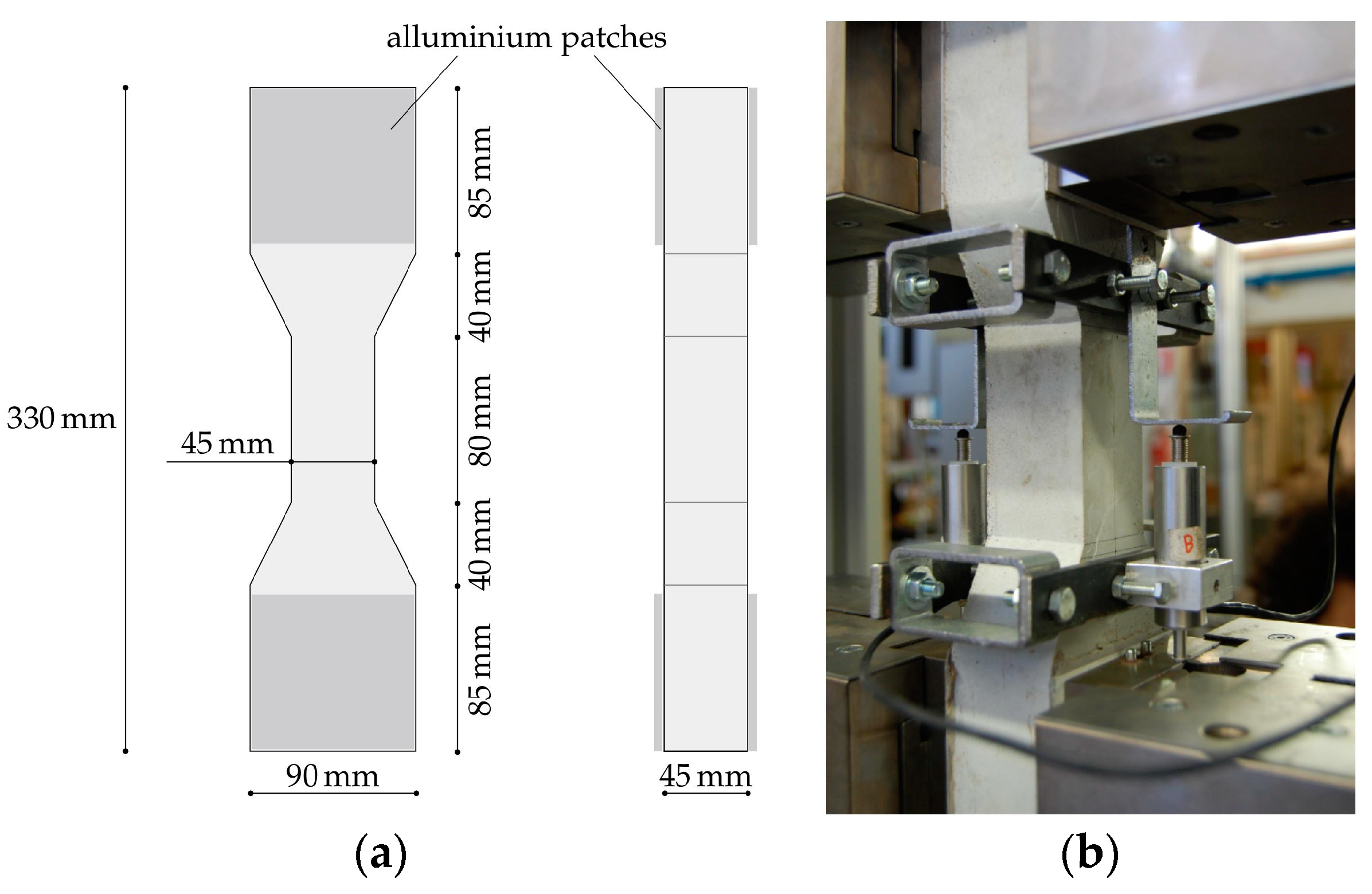
3.1. Experimental Setup

Direct tensile tests have been performed on dog-bone specimens, whose geometry is drawn in Figure 2a. Two fibers percentages, 0.50 and 0.75 vol %, are considered, and three samples are tested for each fibers content. According to the Italian code [16], and in agreement with suggestions of [17], the central cross-section of the sample is a square of side of 45 mm, which is three times the fibers length (i.e., 15 mm) in order to ensure a random fibers distribution. Indeed, anisotropic and not homogeneous fibers distribution leads to a degradation of the mechanical properties of the composite [18,19]. To avoid fibers orientation during the casting procedure, concrete has been spilled by spanning the whole length of the formworks in order to reduce concrete fluxes inducing fibers alignment. Moreover, samples have been only slightly vibrated, again to reduce possible fibers reorientation.
A picture illustrating the tensile test set-up is shown in Figure 2b. Similar set-ups have been recently used to characterize the tensile strength of UHPFRC in [20,21]. Two linear variable differential transformers (LVDT), connected to a custom steel frame, have been used to record the elongation, and also to drive the electro-mechanical testing machine (AllroundLine Zwick Z250 [22], Zwick GmbH & Co. KG, Ulm, Germany). In such a way, an adaptive control is applied to the testing tensile process. A constant elongation rate of 0.0375 s−1 has been applied, corresponding to a displacement rate of 0.05 mm/min. Thin aluminium patches have been glued to the specimen enlargements in order to correct surface imperfections and to improve the transfer of shear stresses. Loading–unloading cycles have been performed during the test, which have allowed to evaluate the plastic strains evolution and the progressive degradation of the stiffness, associated to damage accumulation.

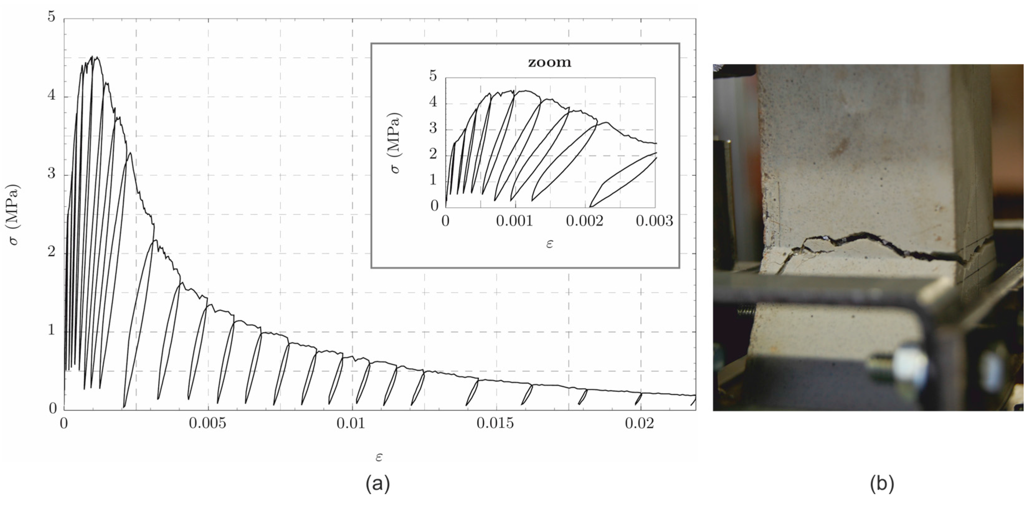
3.2. Experimental Results

Samples with 0.75 vol % of fibers have exhibited a tensile strength considerably larger than samples with 0.50 vol %. Thus, in the following, we just present results on the former, more performant, composite. The stress–strain curve obtained from tensile tests is plotted in Figure 3a, where an enlargement of the initial part of the curve is included. As in [7], three different consecutive stages can be recognized, namely: (1) an initial, very short, linear elastic stage; (2) a short hardening phase, which lasts when the stress peak σ = 4.5 MPa is reached. At the end of the hardening stage, a distinct fracture in the concrete matrix appears, which produces a significant stiffness reduction (up to six times the initial stiffness, and even more); (3) from here on in, the sample experiences a long softening phase, dominated by plastic deformations, which are attributed to fibers yielding, on one side, and to fibers debonding from matrix, on the other side. Finally, the sample fails when fibers are totally pulled out from the concrete matrix. As shown in the picture of Figure 3b, crack forms at the lower cross-section of the narrow central part of the sample.

4. Finite Element Modelling

4.1. Numerical Model

Numerical analysis is performed by implementing the Concrete Damage Plasticity constitutive model (CDP), available in Abaqus. Accounting for plasticity and damage, CDP model is able to reproduce failure processes usually observed in quasi-brittle materials, as concretes. In FRC, breaking is anticipated by an extended stress-softening process, where stiffness degradation combines with plastic deformations.
The basic ingredients of the model are presented in the following. The independent variables are the displacement field u (x,t), the plastic strain tensor εp (x,t), and the damage d (x,t), which is a scalar field varying in [0,1]: d = 0 means sound material, and d = 1 means totally broken material. Space position and time instants are indicated by x and t. The stress tensor is defined as
σ = ( 1 d ) C ( ε ε p ) ,   with   ε = s y m u ,
where C is the elasticity tensor, assumed to be isotropic. The evolution of the plastic deformation is governed by the equations:
ε ˙ p = λ ˙ g p ( σ ¯ ) σ ¯ ,
ε ˜ ˙ p = h ( σ ¯ ) ε ˙ p ,
λ ˙ 0 ,
f p ( σ ¯ , ε ˜ p ) 0
λ ˙ f p ( σ ¯ , ε ˜ p ) = 0
which are written in terms of the effective stress σ ¯ = C ( ε ε p ) . The scalar ε ˜ p is the hardening variable. In the Kuhn–Tucker set of Equations (2c)–(2e), the yield function f p ( σ ¯ , ε ˜ p ) is the one proposed in [23], and modified in [24]. The flow rule (2a) is non-associated, and the Drucker–Prager hyperbolic flow potential is assigned to g p ( σ ¯ ) . In the evolution law (2b), h ( σ ¯ ) is a weighted function of the principal effective stresses. We refer to [10] for the explicit expressions of f p , g p and h .
The evolution of the degradation variable d is governed by an algebraic equation d = d ( σ ¯ , ε ˜ p ) , which, in the simplest one-dimensional case of pure tension has the expression d = 1 σ ¯ / σ M , with σ M the maximum tensile stress (see next Figure 3).
The constitutive parameters to be assigned in the model are: the Young’s modulus E = 42 GPa, the Poisson’s ratio ν = 0.25, and the tensile and compressive stress–strain curves plotted in Figure 4. The tensile curve of Figure 4a coincides with the experimental curve of Figure 3, while the compressive curve of Figure 4b is given by pure compression tests performed on cubic samples, not reported in this paper for brevity.
Three-dimensional simulations have been performed to reproduce the experimental results of tensile tests, while two-dimensional shell elements have been used to model the table. In both cases, numerical analysis has been conducted by implementing the modified Riks method [25,26,27], which, basically, considers the size of the loading step as an additional variable. Incorporated into a Newton–Raphson scheme, the Riks method is particularly suitable to solve non-linear problems where stress-softening processes of strain and damage localization could induce numerical instabilities.
In the next Section 4.2, the experimental tensile test of Section 3 is reproduced by a three-dimensional numerical simulation, and, in Section 4.3, the mechanical response of the Nervi table is investigated for different loading conditions and different boundary conditions. Both table top and legs are modelled as two-dimensional shells. The numerical results presented in the following are partially taken from [28].

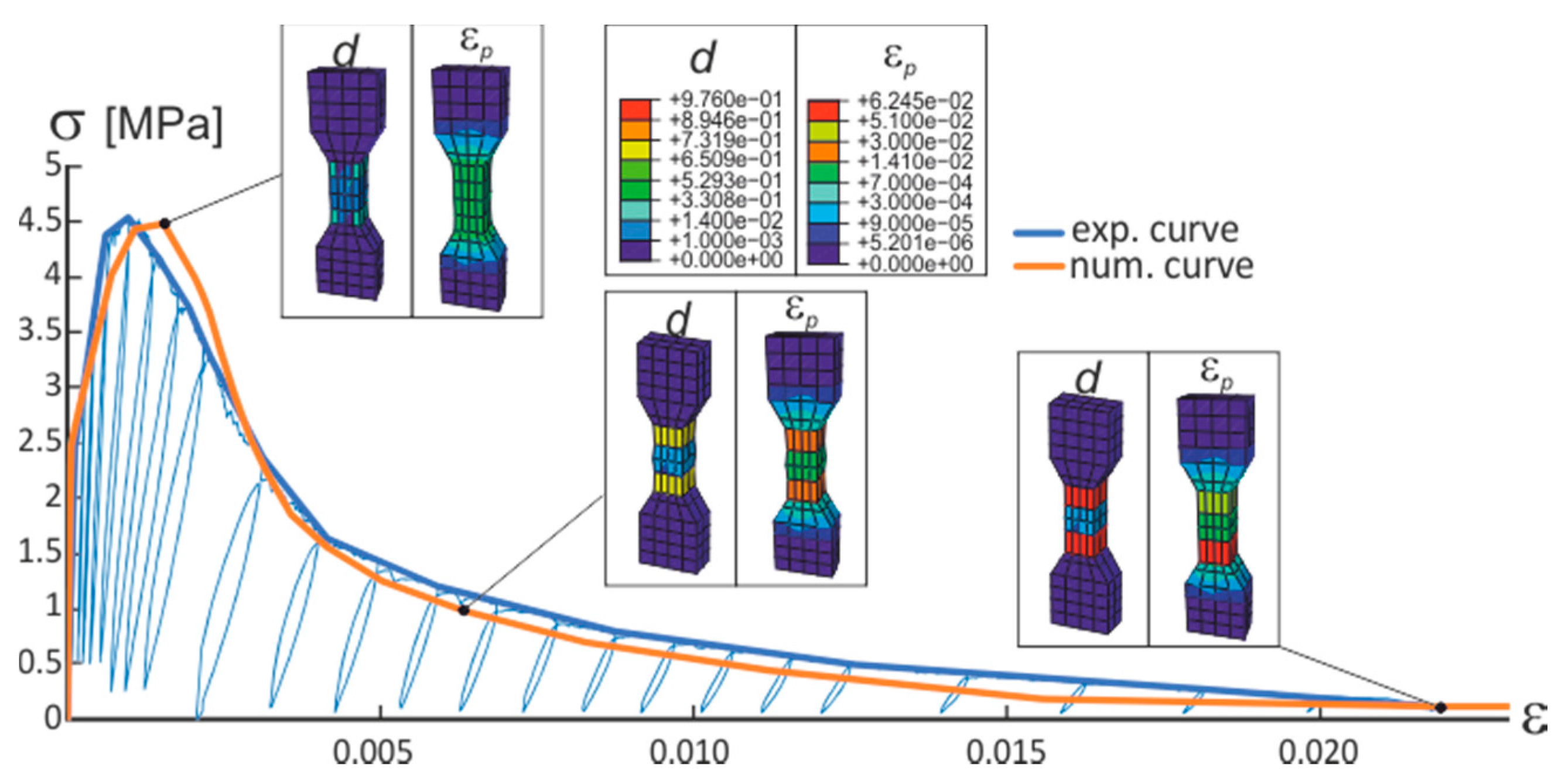
4.2. Simulations: Tensile Tests

The geometry of the dog-bone sample of Figure 2a is discretized by 8-node linear finite elements, with characteristic size equal to 2.25 mm. Since the model is local, the size of the finite elements is related to the size of the so-called process zone, that is the zone where damage localizes at fracture. We have chosen a size equal to 1.5 times the length of fibers. In order to be the material internal length independent from the finite elements size a non-local approach must be followed (see, for instance the variational model [29]).
The sample lower end-section is fixed, and a tensile displacement is applied to the upper end-section. The normal stress σ is given by the reactive normal force at the sample end-sections divided by the section area, and tensile strain ε is measured in the central part of the sample, by considering a measuring base equal to 10.7 cm, as in experiments.
The numerical stress–strain curve is drawn in Figure 5, and compared with the experimental curve. The closeness between curves is quite expected, since the experimental curve has been assigned as input data in the numerical model, and the accuracy of the results just validates the model, and proofs its correctness. More unexpected is the numerical prediction of the failure process, very adherent to the one observed in experiments. In both the two cases, rupture localizes at the extremity of the thinner central part of the sample. A picture of the crack observed in the experiment is reported in Figure 3b, while, as regards numerical simulation, failure evolution is described by the snapshots of damage d and normal plastic strain εp at three different instants, plotted in Figure 5b. At the end of the stress-hardening phase, damage and plastic strain are mainly homogeneously distributed in the narrow central part of the sample (first pair of snapshots). In the subsequent stress-softening stage, they initially localize at the two extremities of the central zone (second pair of snapshot), and then they concentrate (mainly the plastic strains) on the lower extremity of the sample central part, where the sample breaks (third pair of snapshots).

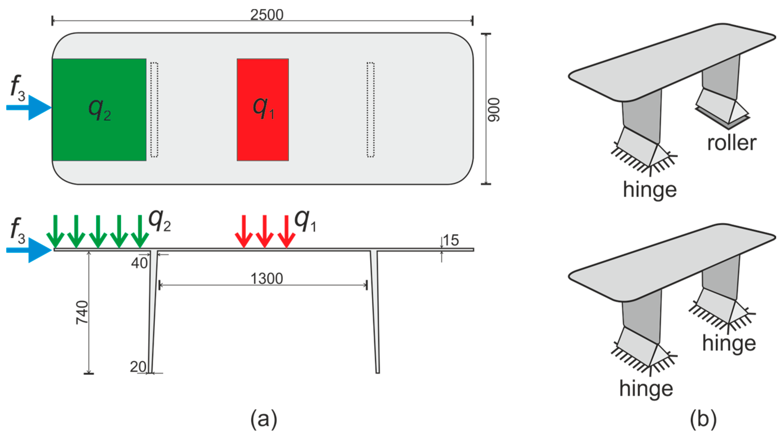
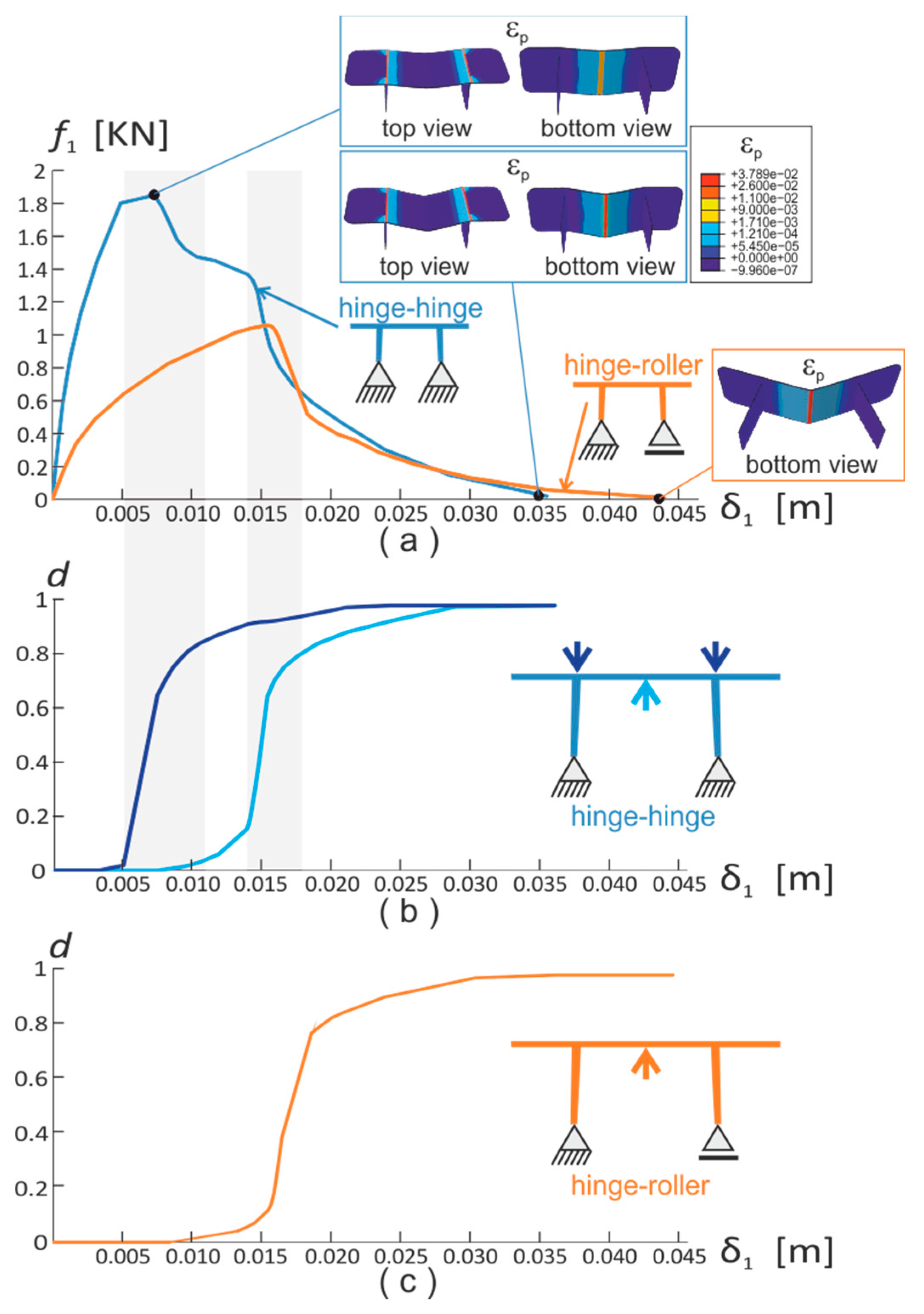
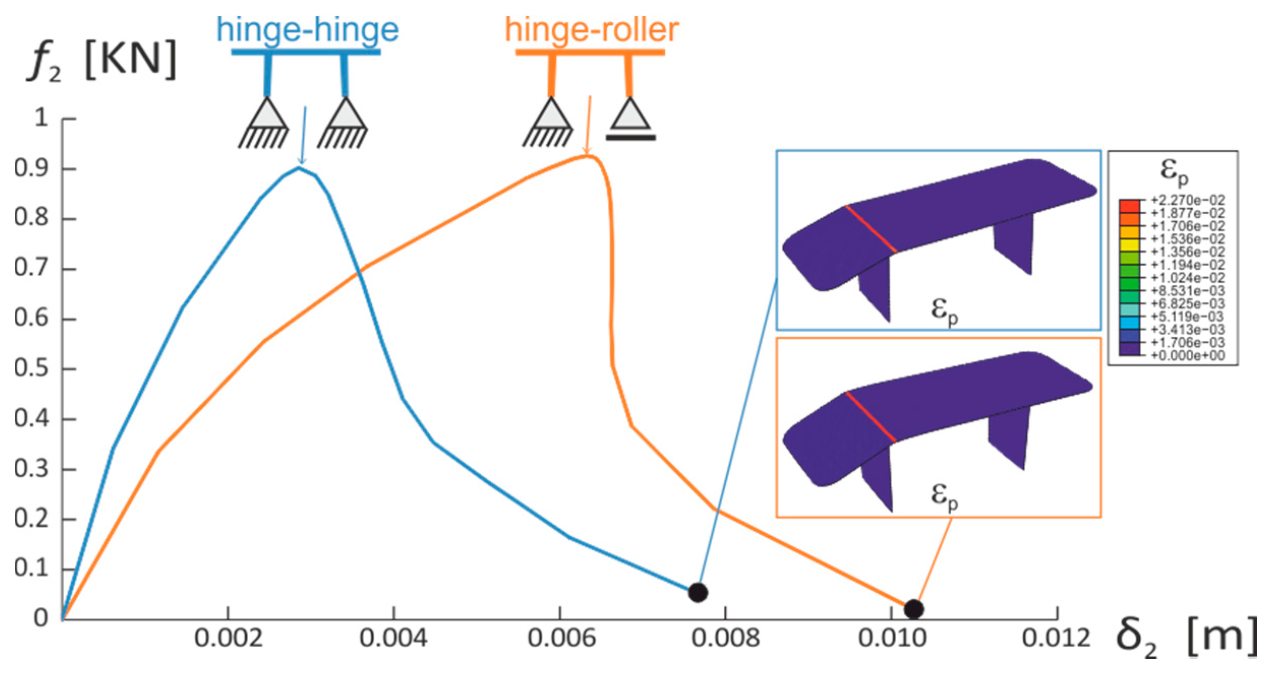
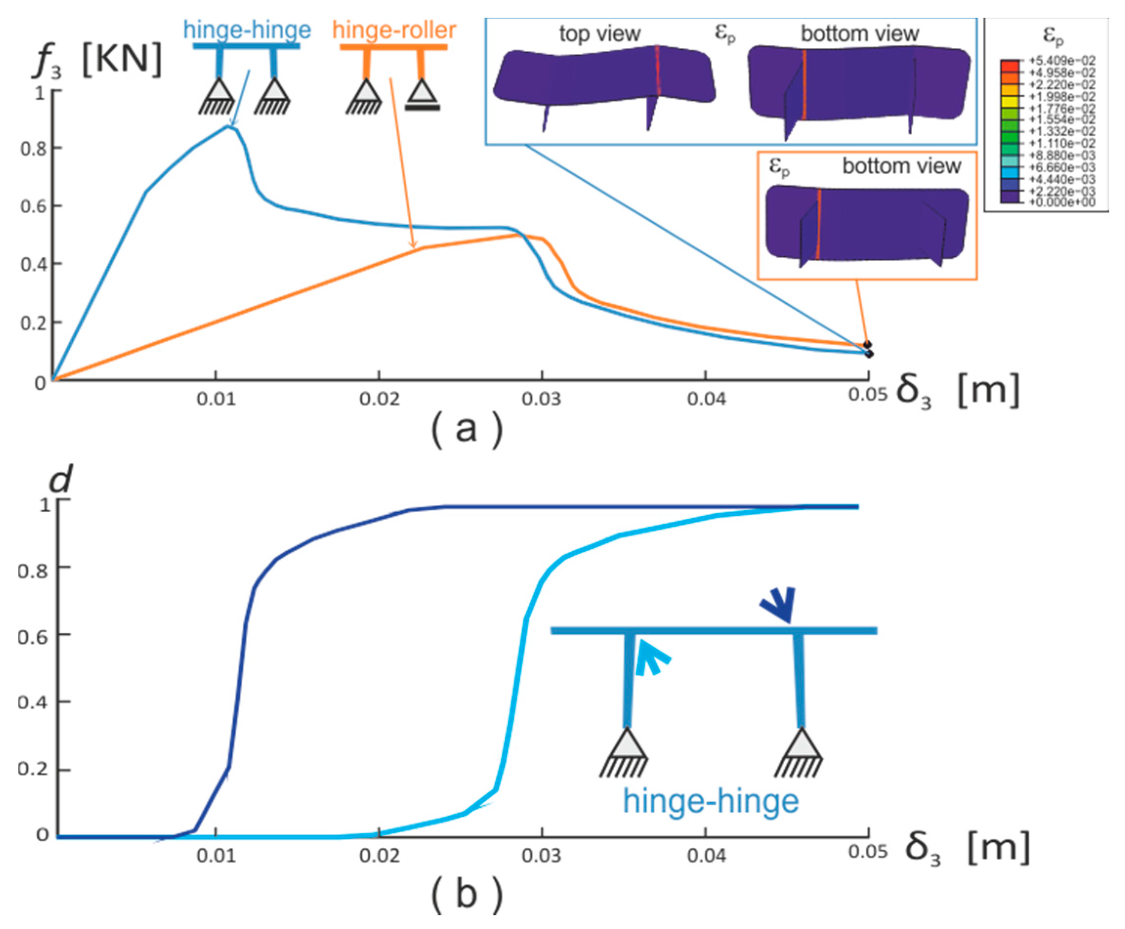
4.3. Simulations: Nervi Table

The Nervi Table (see Figure 1) is studied in this subsection. Its geometry is drawn in Figure 6a. The table top is 2500 × 900 mm2, 15 mm in thickness, with span between legs equal to 1300 mm. Legs are two-dimensional slabs slightly sloped with respect to the vertical direction, whose thickness varies from 20 mm (at the foot) to 40 mm (at the top). Table top and legs are discretized by means of two-dimensional shell elements (4-node S4R elements), whose characteristic size is 2.25 cm. Three different loading conditions are assumed, as schematized in Figure 6a: (i) vertical load q1 applied on a rectangle in the middle of the top (red arrows, and red area); (ii) vertical load q2 applied on a rectangle on the left side of the top (green arrows, and red area); (iii) horizontal force f3 applied in the middle of the top left side (blue arrow). The evolution problem is determined by imposing the load and controlling the displacement of the so-called control points, which are the midpoints of the loading areas (red and green areas in Figure 6) when loads q1 and q2 are applied, and the force application point in the case of f3. The advantage of adopting displacement control is that even softening regimes can be captured. For each loading condition, two different boundary conditions are applied at the foot of the table legs, laid on a horizontal plane: hinge-roller (h-r) conditions and hinge-hinge (h-h) conditions, as schematized in Figure 6b. Inertial forces are always considered. The table weight is 135 kg.
(i) Central vertical loading.
When load q1 is applied, the table behaves as shown in Figure 7. Force f1 = A1q1 (A1 is the area of the loading surface) versus the vertical displacement δ1 of the top central point is plotted in Figure 7a, for h-r and h-h boundary conditions. Both the two curves exhibit an initial hardening phase, and a subsequent softening stage.
Hinge-hinge boundary conditions make the system much stiffer than hinge-roller boundary conditions, the hardening branch of the blue curve being much steeper than that of the orange curve. When h-h boundary conditions are applied, the maximum load attained by the structure is about 1.8 kN, and the corresponding displacement is 7 mm, while a smaller maximum load, about 1.0 kN, and a larger corresponding displacement, around 16 mm, are obtained with h-r boundary conditions.
Estimates of the tensile stress in the bottom side of the midsection can be determined by using the Navier’s formula σ = 6 M / ( b h 2 ) , where M is the bending moment in the midsection, and b and h are the table top width and thickness (b = 900 mm, h = 15 mm). The bending moments are assumed to be M = f l / 4 and M = f l / 8 , for the cases of h-r and h-h boundary conditions, respectively. They are the midpoint bending moments of simply supported and fixed supported beams. Thus, the maximum tensile stresses of the midsection are estimated by the formulas
σ h r = 3 2 l b h 2 f 1   ( h r   bc ) ,   σ h h = 3 4 l b h 2 f 1   ( h h   bc )
If the geometrical dimensions of the Nervi table are considered (see Figure 6), Formula (3) specializes as follows: σ h r = 9.6 f 1 [MPa], and σ h h = 4.8 f 1 [MPa], with f1 measured in kN. The maximum stresses corresponding to the peak values of f1 are σhr = 10.1 MPa and σhh = 8.9 MPa, which are very close to each other. They are about two times larger than the maximum stress given by simple tensile tests (Figure 5). These results are in agreement with experimental evidences [30], according to which the maximum normal stress attained in bending tests is 2–3 times larger than that of pure tensile tests.
In the softening phase, the evolution of plastic strain and damage is quite different in the two cases. Snapshots of the plastic deformation εp are plotted in Figure 7a, and evolution of damage in specific points of the table top is described by the d-δ curves of Figure 7b,c. The points of the table top where damage is registered are indicated by arrows in the table sketches on the right sides of Figure 7b,c. For h-r boundary conditions, εp and d form and grow in a narrow strip in the bottom central part of the top, and, at the end, the top midsection breaks. More involved is the failure process observed when h-h boundary conditions are applied. Indeed, two drops with steep decreasing slope can be clearly observed in the blue softening branch of Figure 7a: the first drop corresponds to damage formation at the extrados of the top, right above the legs, and the second drop corresponds to damage evolution in the bottom midsection of the top. Plastic deformations undergo a similar two-step evolution process, first growing in the top over the legs, and then in the middle. Ultimately, the table top fails in three sections: those adjacent to the legs and the midsection.
(ii) Lateral vertical loading.
The mechanical response to the vertical load q2, applied on the left side of the top (green arrows in Figure 6), is shown in Figure 8. Force-displacement curves are drawn in the case of h-r and h-h boundary conditions, where f2 = A2q2, with A2 the area of the green surface of Figure 6, and δ2 is the vertical displacement of the green surface midpoint. Both the two curves exhibit a maximum load slightly smaller than 1 KN, but the corresponding displacements are different. Indeed, for h-r boundary conditions, the displacement δ2 = 6.5 mm is about two times larger than the displacement obtained with h-h boundary conditions.
The largest stresses are attained on the table top cross-section, placed over the left leg. They can be estimated by means of Navier’s formula, assuming the scheme of a cantilever beam with a uniform distributed loading. Accordingly, the stress on the upper side of the cantilever fixed end section is σ = 3 l ^ f 2 / ( b h 2 ) , where l ^ = 600 mm is the length of the cantilevered portion of the table top. For the Nervi table geometry, the above formula assumes the expression σ = 8.9 f 2 [MPa], with f2 measured in kN. The maximum stress value σ = 8.9 MPa, corresponding to the peak value of f2 = 1 KN, is consistent with the values found in the above point (i).
In the two cases, plastic deformations form in the upper side of the table top, above the left leg (see snapshots in Figure 8), and they lead to the subsequent table failure.
(iii) Horizontal load.
Now the horizontal force f3 applied in the middle of the left side of the table top (see blue arrow in Figure 6) is considered. Force-displacement curves are plotted in Figure 9, with δ3 the horizontal displacement of the application point of f3. As in the previous cases, the larger maximum force is obtained when h-h boundary conditions are applied.
Failure mechanisms depend on the boundary conditions. Indeed, in the case of h-h boundary conditions, plastic strain and damage localize in a narrow strip in the bottom side of the table top, closed to the left leg (see the snapshot in the orange frame of Figure 9a). For h-h boundary conditions, the softening phase undergoes two stages, corresponding to the two drops down of the softening response curve. In the first one, damage localizes near the right leg, in the upper side of the table top, while, in the second one, damage evolves near the left leg, in the lower side. This is clearly shown by the d3 curve of Figure 9b. First damage forms at the extrados close to the left leg, and then at the intrados near the right leg, where the largest tensile stresses are attained.
If h-r boundary conditions are considered, the largest stresses are registered at the upper section of the table left leg. The maximum stress in this section can be estimated by the formula σ = 6 l ˜ f 3 / ( b ˜ h ˜ 2 ) , where l ˜ = 740 mm, b ˜ = 560 mm, and h ˜ = 20 mm are the length, the width and the thickness of the table legs, respectively. This formula is obtained by supposing the leg to be a cantilever subjected to a load on its free end section, and using Navier’s formula. For the Nervi table geometry, the above formula rewrites σ = 19.8 f 3 [MPa], with f3 measured in kN. The peak stress is σ = 9.9 MPa, corresponding to the peak force f2 = 0.5 KN.
Finally, we notice that in all the performed simulations, damage and plastic strains are always induced by tensile stress states, and that the material remains linearly elastic when subjected to compressive stresses.
To conclude this section, we present some results of simulations, where geometrical and material parameters are enhanced in order to improve the strength of the table. The geometry is modified by increasing the table top thickness from 15 mm to 20 mm, and the material is improved by considering larger maximum tensile stress (σM,t in Figure 4a), i.e., σM,t = 5.6 MPa and σM,t = 7.0 MPa. The resulting f11 curves, obtained when the load q1 is applied, and h-r boundary conditions are assigned, are plotted in Figure 10, and compared with the curve (green line) of simulation described at point (i). When the top thickness is increased (orange curve), the maximum load doubles, reaching the peak value of 2 KN. However, besides the strength improvement, increased thickness produces undesired weight growth (from 135 kg to 160 kg). On the other hand, more performant concretes contribute to increase the peak load of about 25% and 50%, for σM,t = 5.6 MPa and σM,t = 7.0 MPa, respectively. In this respect, ongoing mix design studies are conducted, aimed at improving the mechanical properties, on one side, and at guaranteeing workability and surface fineness, on the other side.

5. Conclusions

The feasibility study of a table made of fiber-reinforced concrete was proposed. It has required different contributions, coming from different fields. At first, the expertise of designers was needed to conceive shape and geometry of the table: the so-called Nervi table was proposed. In a second step, the table, taken as a structure in itself, was subjected to an engineering process. Notice that cooperation between designers and structural/material engineers is very uncommon, and thus it constitutes one of the novelty elements of the proposed study.
The engineering process was conducted in three phases:
(i)
development of a fiber-reinforced concrete with specific properties, that is, large workability, very low surface roughness, and large mechanical strength to tensile stresses;
(ii)
experimental testing, to characterize the material mechanical properties, and to calibrate the numerical model;
(iii)
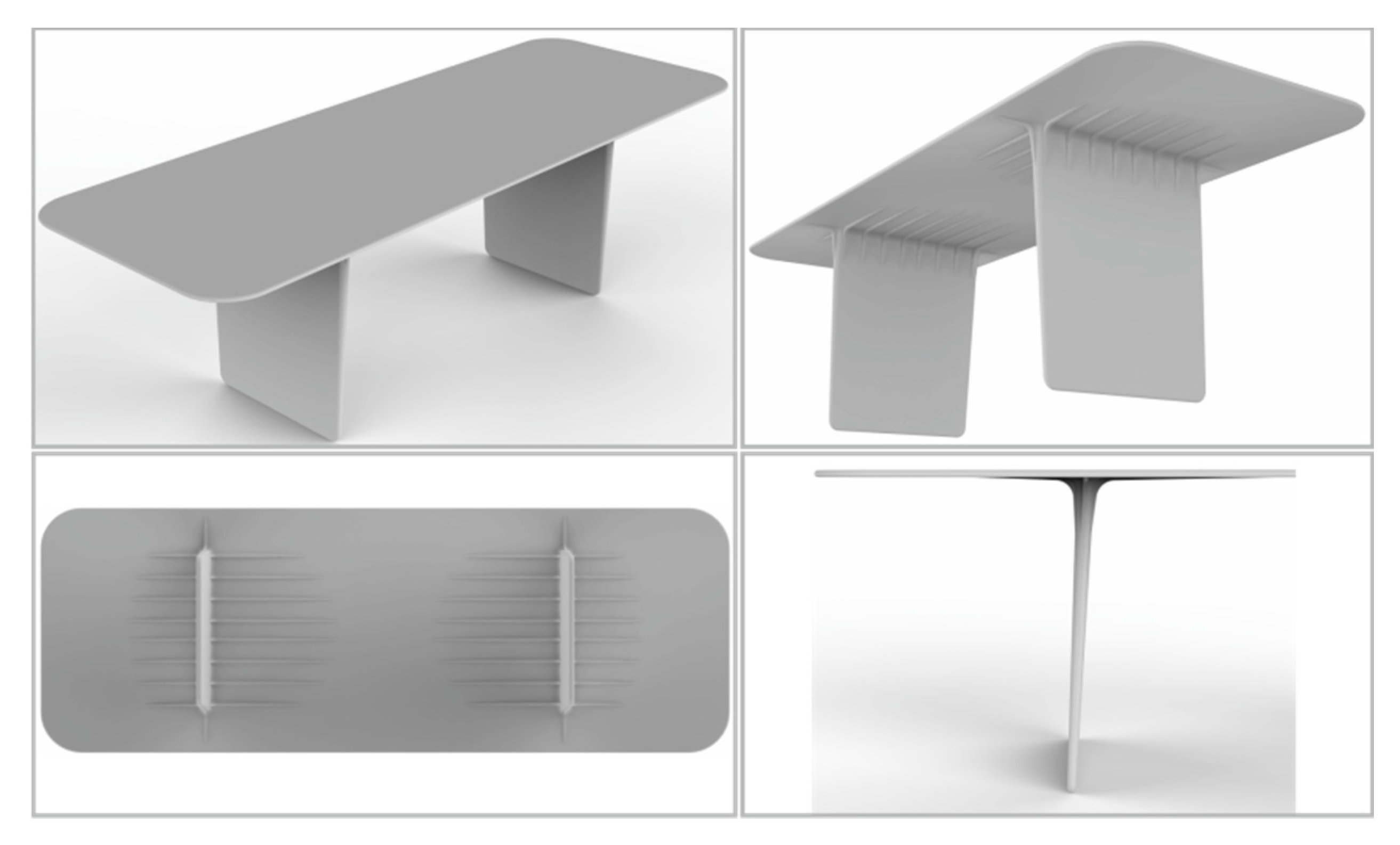
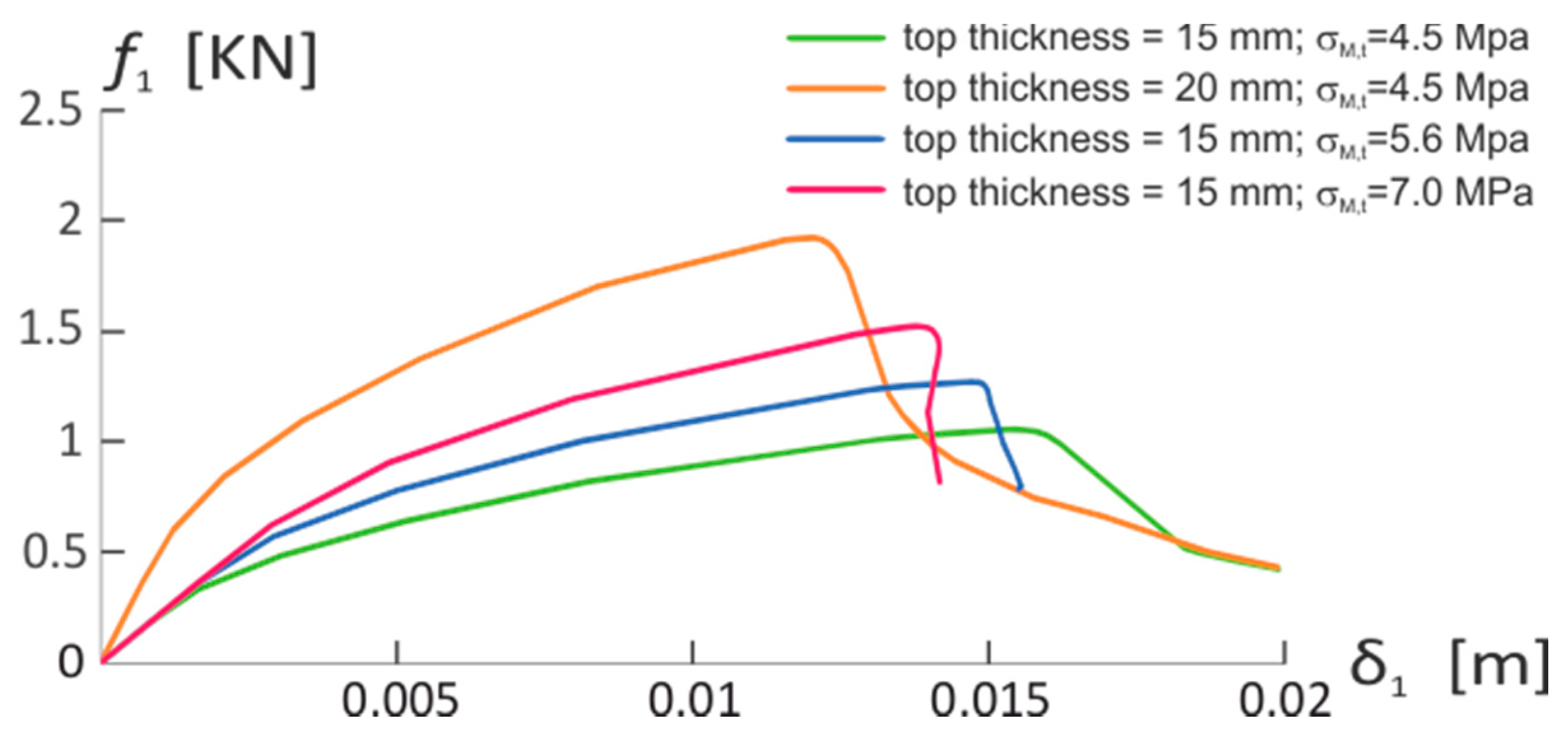
numerical analysis, where accurate numerical simulations were conducted in order to determine the table capability of bearing different loadings, under different boundary conditions. It was found that the worst mechanical responses are registered when the table is simply supported over a horizontal surface. In this case, the maximum vertical and horizontal loads, that lead to the table collapse, are around 0.9–1.0 KN and 0.5–0.6 KN, respectively. Furthermore, it was found that the most stressed cross-sections of the table top, where damage and plastic strains localize, are the midsection and the sections adjacent to the supporting legs. Localized inelastic phenomena initiates when the stress σ = 9–10 MPa is reached, which represents the maximum stress that concrete can sustain under bending loadings, and it is two times larger than the maximum stress of pure tensile tests. Analogous differences were found in experimental studies (see [30]). This suggests to reinforce the table top in these sections, and, in this regard, the ribs at the intrados of the Nervi table (see Figure 1), adjacent to the legs, represent useful strengthening elements.
Different proposals for enhancing the mechanical performances of the table were analyzed, such as geometrical changes (larger thicknesses of the table top), and material enhancements (augmented tensile strengths). It was found that modest increments of the above-mentioned parameters produce appreciable mechanical improvements. Thus, on the basis of this analysis, future work will be devoted (i) to found more appropriate geometries of the table top, supposing, for instance, variable cross-sections, and (ii) to develop more performing fiber-reinforced concretes, with optimized mix design.

Acknowledgments

We thank Stefano Vidoli and Vittorio Dragone, from the Dipartimento di Ingegneria Strutturale e Geotecnica, Università di Roma “La Sapienza”, for their valuable support and assistance in performing tensile tests.

Author Contributions

Robin Rizzini/Metrica provided the Nervi table design; Valeria Corinaldesi developed the fiber-reinforced concrete conceived for the table; Roberto Alessi designed and carried out tensile tests; Elisa Baioni and Giovanni Lancioni performed the numerical analyses. All authors have read and approved the final manuscript.

Conflicts of Interest

The authors declare no conflict of interest.

References

  1. Swamy, R.N. Fiber Reinforced Cement and Concrete. In Proceedings of the 4th RILEM International Symposium, Sheffield, UK, 20–23 July 1992. [Google Scholar]
  2. Cheyrezy, M.; Deniel, J.I.; Krenciel, H.; Mihashi, H.; Pera, J.; Rossi, P.; Xi, Y. Specific Production and manufacturing issue. In High Performance Fiber Reinforced Cement Composite, Proceedings of the 2nd International Workshop (HPFRCC2), Ann Arbor, MI, USA, 11–14 June 1995; Naaman, A.E., Reinhardt, H.W., Eds.; E.&F.N. Spon: London, UK, 1995; Volume 2, pp. 25–41. [Google Scholar]
  3. Di Prisco, M.; Plizzari, G.; Vandewalle, L. Fibre reinforced concrete: New design perspectives. Mater. Struct. 2009, 42, 1261–1281. [Google Scholar] [CrossRef]
  4. Park, S.H.; Kim, D.J.; Ryu, G.S.; Koh, K.T. Tensile behavior of Ultra High Performance Hybrid Fiber Reinforced Concrete. Cem Concr. Compos. 2012, 34, 172–184. [Google Scholar] [CrossRef]
  5. Wille, K.; El-Tawil, S.; Naaman, A.E. Properties of strain hardening ultra high performance fiber reinforced concrete (UHP-FRC) under direct tensile loading. Cem. Concr. Compos. 2014, 48, 53–66. [Google Scholar] [CrossRef]
  6. Yu, R.; Spiesz, P.; Brouwers, H.J.H. Mix design and properties assessment of Ultra-High Performance Fibre Reinforced Concrete (UHPFRC). Cem. Concr. Compos. 2014, 56, 29–39. [Google Scholar] [CrossRef]
  7. Jungwirth, J.; Muttoni, A. Structural behavior of tension members in UHPC. In Proceedings of the International Symposium on UHPC 2004, Kassel, Germany, 13–15 September 2004; pp. 1–12. [Google Scholar]
  8. Gosselin, C.; Duballet, R.; Roux, P.; Gaudillière, N.; Dirrenberger, J.; Morel, P. Large-scale 3D printing of ultra-high performance concrete—A new processing route for architects and builders. Mater. Des. 2016, 100, 102–109. [Google Scholar] [CrossRef]
  9. Website Kristalia srl. Available online: www.kristalia.it/design-tables/boiacca/outdoor-concrete-table/ (accessed on 1 January 2013).
  10. Abaqus Theory Manual, Version 6.10; Dassault Systèmes Simulia Corp.: Providence, RI, USA, 2010.
  11. Collepardi, M. The New Concrete; Grafiche Tintoretto: Villorba (Treviso), Italy, 2006. [Google Scholar]
  12. Corinaldesi, V.; Nardinocchi, A.; Donnini, J. The Influence of Expansive Agent on the Performance of Fiber Reinforced Cement-Based Composites. Constr. Build. Mater. 2015, 91, 171–191. [Google Scholar] [CrossRef]
  13. Corinaldesi, V.; Nardinocchi, A. Mechanical characterization of Engineered Cement-based Composites prepared with hybrid fibres and expansive agent. Compos. Part B Eng. 2016, 98, 389–396. [Google Scholar] [CrossRef]
  14. Corinaldesi, V.; Donnini, J.; Nardinocchi, A. The Influence of Calcium Oxide Addition on Properties of Fiber Reinforced Cement-Based Composites. J. Build. Eng. 2015, 4, 14–20. [Google Scholar] [CrossRef]
  15. Corinaldesi, V.; Nardinocchi, A. Influence of type of fibers on the properties of high performance cement-based composites. Constr. Build. Mater. 2016, 107, 321–331. [Google Scholar] [CrossRef]
  16. CNR. Istruzioni per la Progettazione, l’Esecuzione ed il Controllo di Strutture di Calcestruzzo Fibrorinforzato. Technical Report; Consiglio Nazionale delle Ricerche: Rome, Italy, 2006. [Google Scholar]
  17. Akita, H.; Koide, H.; Mihashi, H. Specimen Geometry in Uniaxial Tension Test of Concrete; FraMCoS-6; Carpinteri, A., Ed.; Taylor & Francis: London, UK, 2007. [Google Scholar]
  18. Bensaid Boulekbache, B.; Hamrat, M.; Chemrouk, M.; Amziane, S. Flowability of fibre-reinforced concrete and its effect on the mechanical properties of the material. Constr. Build. Mater. 2010, 24, 1664–1671. [Google Scholar] [CrossRef]
  19. Herrmann, H.; Lees, A. On the influence of the rheological boundary conditions on the fibre orientations in the production of steel fibre reinforced concrete elements. Proc. Estonian Acad. Sci. 2016, 65, 408–413. [Google Scholar] [CrossRef]
  20. Choi, J.I.; Lee, B.Y.; Ranade, R.; Li, V.C.; Lee, Y.; Composites, C.; York, N. Ultra-high-ductile behavior of apolyethylene fiber-reinforced alkali-activated slag-based composite. Cem. Concr. Compos. 2016, 70, 153–158. [Google Scholar] [CrossRef]
  21. Paschalis, S.A.; Lampropoulos, A.P. Ultra-high-performance fiber-reinforced concrete under cyclic loading. ACI Mater. J. 2016, 113, 419–427. [Google Scholar] [CrossRef]
  22. Zwick/Roell. AllroundLine Z250 SW Materials Testing Machines. Available online: https://www.zwick.com/en/universal-testing-machines/allroundline-test-machine (accessed on 2017).
  23. Lubliner, J.; Oliver, J.; Oller, S.; Onate, E. A Plastic-Damage Model for Concrete. Int. J. Solids Struct. 1989, 25, 299–329. [Google Scholar] [CrossRef]
  24. Lee, J.; Fenves, G.L. Plastic-Damage Model for Cyclic Loading of Concrete Structures. J. Eng. Mech. 1998, 124, 892–900. [Google Scholar] [CrossRef]
  25. Ramm, E. Strategies for Tracing the Nonlinear Response Near Limit Points, Nonlinear Finite Element Analysis in Structural Mechanics; Wunderlich, E., Stein, E., Bathe, K.J., Eds.; Springer-Verlag: Berlin, Germany, 1981. [Google Scholar]
  26. Crisfield, M.A. Snap-Through and Snap-Back Response in Concrete Structures and the Dangers of Under-Integration. Int. J. Numer. Methods Eng. 1986, 22, 751–767. [Google Scholar] [CrossRef]
  27. Powell, G.; Simons, J. Improved Iterative Strategy for Nonlinear Structures. Int. J. Numer.Methods Eng. 1981, 17, 1455–1467. [Google Scholar] [CrossRef]
  28. Baioni, E. Plasticity and Fracture Models for the Study of High Performance Fibre-Reinforced Concretes: Numerical Applications to Design Objects, Master Degree Thesis in Building Engineering; Università Politecnica delle Marche: Piazza Roma, Italy, 2017. [Google Scholar]
  29. Lancioni, G.; Corinaldesi, V. Variational modelling of diffused and localized damage with applications to fiber-reinforced concretes. Meccanica 2017. [Google Scholar] [CrossRef]
  30. Maca, P.; Savjac, R.; Vavrinik, T. Experimental investigation of mechanical properties of UHPFRC. Proc. Eng. 2013, 65, 14–419. [Google Scholar] [CrossRef]
Figure 1. Nervi Table renderings.
Technologies 05 00041 g001
Figure 2. (a) Dog-bone specimen geometry; (b) experimental set-up of a tensile test.
Technologies 05 00041 g002
Figure 3. (a) Experimental stress–strain curve from tensile tests. (b) Picture of the cracked sample.
Technologies 05 00041 g003
Figure 4. Tensile (a) and compressive (b) response curves.
Technologies 05 00041 g004
Figure 5. σ–ε numerical and experimental curves. Three snapshots of damage d and normal plastic strain εp fields at different instants of the deformation process.
Technologies 05 00041 g005
Figure 6. (a) Table geometry and loading conditions. (b) Boundary conditions.
Technologies 05 00041 g006
Figure 7. Central vertical loading. (a) Force-displacements curves for different boundary conditions, and snapshots of plastic strains. (b,c) Damage-displacement curves evaluated in different points of the table, when hinge-hinge (b) and hinge-roller (c) boundary conditions are assigned.
Technologies 05 00041 g007
Figure 8. Lateral vertical loading. Force-displacements curves for different boundary conditions, and snapshots of plastic deformation at failure.
Technologies 05 00041 g008
Figure 9. Horizontal loading. (a) Force-displacement curves for different boundary conditions, and snapshots of plastic deformation at failure. (b) Damage displacement curves evaluated in different points of the table, when hinge-hinge boundary conditions are applied.
Technologies 05 00041 g009
Figure 10. Force-displacement curves for different thicknesses of the table top and different maximum tensile stress σM,t (see Figure 4).
Technologies 05 00041 g010

