Performance Comparison of WiFi and UWB Fingerprinting Indoor Positioning Systems

Abstract

Ultra-wideband (UWB) and WiFi technologies have been widely proposed for the implementation of accurate and scalable indoor positioning systems (IPSs). Among different approaches, fingerprinting appears particularly suitable for WiFi IPSs and was also proposed for UWB IPSs, in order to cope with the decrease in accuracy of time of arrival (ToA)-based lateration schemes in the case of severe multipath and non-line-of-sight (NLoS) environments. However, so far, the two technologies have been analyzed under very different assumptions, and no fair performance comparison has been carried out. This paper fills this gap by comparing UWB- and WiFi-based fingerprinting under similar settings and scenarios by computer simulations. Two different k-nearest neighbor (kNN) algorithms are considered in the comparison: a traditional fixed k algorithm, and a novel dynamic k algorithm capable of operating on fingerprints composed of multiple location-dependent features extracted from the channel impulse response (CIR), typically made available by UWB hardware. The results show that UWB and WiFi technologies lead to a similar accuracy when a traditional algorithm using a single feature is adopted; when used in combination with the proposed dynamic k algorithm operating on channel energy and delay spread, UWB outperforms WiFi, providing higher accuracy and more degrees of freedom in the design of the system architecture.

1. Introduction

Information on the position of wireless devices may help the implementation of next-generation communication systems, infrastructures and services [1,2]. The design of accurate and scalable indoor positioning systems (IPSs), aiming at extending outdoor location-based services, provided by systems such as GPSs, to indoor environments, is thus very appealing [3]. Among the investigated techniques and technologies, ultra-wideband (UWB) and WiFi are two major candidates for implementing reliable IPSs [4,5].

Typically, UWB IPSs are based on triangulation principles applied to dedicated infrastructures formed by anchor nodes (ANs). Within these systems, the first positioning phase is referred to as ranging, and it estimates the distances between each AN and a device in the unknown position, referred to in the following as a target node (TN), through either lateration techniques, such as time of arrival (ToA) and time difference of arrival (TDoA), or through the received signal strength (RSS); the estimate of the TN position is then obtained by exploiting the ranging phase results, through either geometric or linear and non-linear least squares minimization approaches [4]. It is demonstrated that these schemes are highly accurate when line-of-sight (LoS) and perfect time synchronization conditions are verified between ANs and the TN; however, several factors, such as (a) direct path excess-delay/blockage due to non-LoS (NLoS) propagation; (b) clock drifts due to asynchronism; and (c) interference from other users/networks, lead to a significant decrease in accuracy, as a result of their negative impact on the ToA estimation [6,7]. In order to cope with the decrease in accuracy of lateration techniques, the application of the fingerprinting approach has been recently proposed for UWB [8,9,10,11,12,13,14]; in general, fingerprinting relies on two phases: the first, referred to as the offline phase, is a collection of data related to the signal propagation (fingerprints) and with respect to predefined reference node (RN) positions in the area of interest. During the second phase (online phase), the TN position is estimated through the application of pattern-matching techniques between RNs and TN fingerprints. Several choices are possible for the data to be collected: in the case of UWB, channel impulse response (CIR) location-dependent features have been proposed as fingerprints, because of the possibility of the accurate temporal resolution of multipath components typically forming the CIR [15]. In parallel, in the view of the cost-effective reuse of pre-existing communication infrastructure, fingerprinting emerges as one of the most appealing solutions in the case of WiFi-based IPSs [5]; in this case, the use of WiFi access points (APs) as ANs and the collection of RSS values in the RN positions have been widely proposed and analyzed [16,17,18,19,20,21].

UWB can be expected to provide better accuracy than WiFi, because of its larger bandwidth and consequently lower bounds on the positioning error [6,22]. However, no performance comparison has been carried out so far in order to quantify this improvement; in general, the performance of WiFi and UWB fingerprinting systems has been instead analyzed using very different assumptions, in particular regarding the density of fingerprints and the corresponding measurement effort in the offline phase, which is significantly higher in the case of UWB. The main goal of this work is to fill this gap by providing a comparison, based on simulation, of RSS-based WiFi and CIR-based UWB fingerprinting IPSs, within the same environment and using the same spatial density and thus the same total number of RNs. The two technologies are compared in combination with two different positioning algorithms: a traditional k-nearest neighbors (kNN) scheme with fixed k, and a novel algorithm that adaptively determines k using multiple CIR location-dependent features, in particular, energy and the root-mean-square delay spread (RMS-DS).

The paper is organized as follows: Section 2 reviews related work on WiFi and UWB fingerprinting IPSs, while Section 3 introduces the motivation for the present work and its innovative contributions. Section 4 provides a description of WiFi and UWB systems—in particular, of signal features used to define the fingerprints in the two cases—and of the two positioning algorithms. Section 5 provides details on the common framework used for performance evaluation, while simulation results are reported and discussed in Section 6; finally, Section 7 concludes the paper.

2. Related Work

As mentioned in Section 1, fingerprinting is typically organized into offline and online phases.

Given an area of interest $\mathcal{A}$ and L and N as the total numbers of ANs and RNs, the offline phase consists of the collection of N fingerprints ${\mathit{s}}_n$ (with $n=1,\cdots ,N$), where it is assumed for the moment that the generic lth component $s_{n,l}$ of ${\mathit{s}}_n$ contains a single signal feature extracted in relation to the lth AN (with $l=1,\cdots ,L$); the extension to multiple features is introduced in Section 4. During the online phase, whenever the position of the mth TN has to be estimated, a fingerprint ${\mathit{t}}_m$ is measured and then compared with each ${\mathit{s}}_n$ fingerprint; finally, the TN position is estimated as a function of the positions of the RNs with the most similar fingerprints, where the concept of similarity depends on the collected data and the adopted estimation algorithm. The effective deployment of fingerprinting requires several challenges to be met: (1) the choice of data and technology to be used; (2) the sensitivity of data to signal propagation variability; (3) the efficient planning of the offline phase in terms of AN/RN topologies; (4) the definition and optimization of the positioning algorithm.

RSS-Based WiFi Fingerprinting IPSs—In the context of WiFi fingerprinting IPSs, different aspects have been investigated [5]. In this section, a general system model that is the basis of several proposed solutions is reported.

In a WiFi-based approach, the L ANs are APs continuously transmitting a beacon sequence, while the N RNs are positions being visited by a reference receiver (Rx) while collecting RSS values of beacons and thus defining a RSS fingerprint for each RN. Once the fingerprint for the TN is similarly collected by the target Rx, several approaches might be used for the position estimation; among them, deterministic kNN algorithms are widely investigated, because of the relative ease of implementation. They are based on the definition of a deterministic similarity metric between fingerprints, referred to as $\mathtt{sim}({\mathit{t}}_m,{\mathit{s}}_n)$, and the final estimated position is determined as the average of the k RN positions with the most similar fingerprints:

$${\widehat{\mathit{p}}}_m=\frac{{\sum }_{n=1}^k{\mathit{p}}_n}{k}$$

(1)

where ${\mathit{p}}_n=(x_n,y_n,z_n)$ and ${\widehat{\mathit{p}}}_m=({\widehat{x}}_m,{\widehat{y}}_m,{\widehat{z}}_m)$ are the nth RN position and the estimate of the mth TN, in the three-dimensional (3D) coordinate system defined for $\mathcal{A}$, respectively. Existing WiFi fingerprinting systems using kNN algorithms typically differ under the following two aspects:

• Selection of k: Previous works have showed the impact of the value of k on the positioning accuracy. Existing schemes can be broadly divided into two families: a priori fixed k schemes and dynamic k schemes. In a priori fixed k schemes, k is predefined and does not depend on the positioning request; it has been empirically found that the average positioning error in these schemes is typically minimized by selecting k between 2 and 10 [16,17,18,19]. Dynamic k schemes typically rely on the introduction of a variable threshold in order to determine the value of k depending on the specific positioning request [19,23,24].
• Similarity metric: Different similarity metrics have been proposed [20]. A popular choice is the use of the inverse Minkowski distance with order $o\ge 1$ (orders typically used are $o=1$, i.e., the Manhattan distance, and $o=2$, i.e., the Euclidean distance). Denoting with ${\mathcal{D}}^o({\mathit{t}}_m,{\mathit{s}}_n)$ the Minkowski distance with order o, $\mathtt{sim}({\mathit{t}}_m,{\mathit{s}}_n)$ is then defined as follows:

  $$\mathtt{sim}({\mathit{t}}_m,{\mathit{s}}_n)={[{\mathcal{D}}^o({\mathit{t}}_m,{\mathit{s}}_n)]}^{-1}={\left[{\left(\sum _{l=1}^L{|t_{m,l}-s_{n,l}|}^o\right)}^{\frac{1}{o}}\right]}^{-1}$$

  (2)

CIR-Based UWB Fingerprinting IPSs—While RSS is traditionally used as a signal feature in WiFi IPSs, several location-dependent CIR features are being considered for UWB IPSs.

Before reporting the related work on UWB fingerprinting, similarities and dissimilarities with the WiFi case should be highlighted. On the one hand, differently from the WiFi case, UWB IPSs are mainly designed for transmitter (Tx) localization. For this reason, the L ANs are receivers, while the N RNs are positions being visited by a reference Tx. The fingerprint of the nth RN is then obtained by evaluating the CIRs in the ANs when the reference Tx is beaconing from the nth RN position. On the other hand, similarly to the WiFi case, UWB fingerprinting requires in general no perfect time synchronization between ANs and RNs/TNs during offline/online phases. It is instead required that the Tx placed in the RN/TN transmits the beacon sequence within a predefined observation time $T_{\mathtt{ob}}$, during which the ANs are active. The duration of $T_{\mathtt{ob}}$ should be set in order to include most of the CIR time delay spread, so as to collect most of its multipath components.

Several works propose CIR-based UWB fingerprinting; many of them have introduced the concept of regions, typically of areas in the order of ${\mathtt{cm}}^2$, inside the area of interest $\mathcal{A}$ [8,9,10,11]: once a single Rx is placed in $\mathcal{A}$, an extensive CIR measurement campaign is performed for each region while placing the reference Tx at several RN positions, separated by a few centimeters from each other. The performance analysis has typically focused on evaluating the probability of the correct identification of the region in which the Tx is located. A different approach is proposed in [12,13,14]: several CIR features are considered as possible fingerprints, mainly in conjunction with a neural network-based estimation phase. Among others, two specific CIR features have emerged as preferred choices: CIR energy and RMS-DS. It is interesting to note that the above two features have been also adopted in research works focusing on the identification of UWB CIRs as LoS versus NLoS, which is one of the main challenges in the design of ToA/TDoA-based UWB localization [25,26]. Previous work thus clearly identifies energy and RMS-DS as the most suitable options to represent an UWB CIR; as a result, these were adopted in this work, as detailed in Section 4. In analogy with WiFi, the performance analysis in [12,13,14] was carried out in terms of TN position estimation rather than region identification; however, no performance comparison with WiFi was provided and, as compared to the typical WiFi deployment in the offline phase, much more extensive CIR measurement campaigns were carried out.

3. Motivation and Contribution

As introduced in Section 1 and moving from the observations of Section 2, the main goal of this work is to provide a fair comparison of RSS-based WiFi and CIR-based UWB fingerprinting IPSs, within the same environment and introducing common assumptions and performance targets, in order to verify whether, and to what extent, UWB technology leads to higher positioning compared to WiFi. The following novel contributions can be identified with respect to previous work:

• The two technologies are analyzed in the same scenario in combination with both a fixed kNN algorithm and a novel dynamic kNN algorithm, capable of taking advantage of both monodimensional and multidimensional fingerprints.
• Differently from previous works on UWB fingerprinting [8,9,10,11], no regions are defined in the area of interest, and the positioning accuracy is provided in terms of coordinate estimation.
• Differently from [12,13], the work is based on simulation, allowing us to derive an average performance comparison not depending on a single AN/RN topology, as a result of the randomization of topologies carried out, within the area, through of the adoption of Poisson point processes (PPPs).

4. Fingerprinting Positioning Systems

In this section, a common notation is established in order to describe topologies and system parameters adopted in the analysis of WiFi and UWB positioning systems; furthermore, the algorithms used in the analysis are introduced.

4.1. Notation

In this work, a topology is defined by the numbers and positions of ANs and RNs; in the following, for the generic jth topology, $L_j$ indicates the number of ANs, while $N_j$ indicates the number of RNs. Both systems operate on the basis of fingerprints, with the goal of determining the positions of a set of M TNs: ${\mathit{s}}_n$ (with $n=1,2,\cdots ,N_j$) indicates the fingerprint collected during the offline phase at the position of the nth RN and stored in the system database, while ${\mathit{t}}_m$ (with $m=1,2,\cdots ,M$) indicates the fingerprint collected during the online phase at the unknown position of the mth TN. We note that each fingerprint may in general include a set of $F\ge 1$ features for each AN; the number of ANs $L_j$ and the number of features F thus determines the size of a fingerprint. A fingerprint is in this case defined as ${\mathit{s}}_n=\{{\mathit{s}}_n^1,\cdots ,{\mathit{s}}_n^f,\cdots {\mathit{s}}_n^F\}$, where the fth vector ${\mathit{s}}_n^f$ contains the data related to the fth feature considered in the definition of the fingerprints.

4.2. Definition of Fingerprints

WiFi IPS—For the WiFi-based IPS, a single feature is adopted in defining the fingerprint associated to each RN or TN: the RSS measured at the corresponding position for the signals from the $L_j$ APs. As a result, the fingerprint ${\mathit{s}}_n$ for the nth RN consists of a vector of $1\times L_j$ RSS values; denoting as ${\mathtt{RSS}}^{n,l}$ the RSS for the pair formed by the nth RN and the lth AN, it follows that ${\mathit{s}}_n=({\mathtt{RSS}}^{n,1},\cdots ,{\mathtt{RSS}}^{n,L_j})$. Similarly, the fingerprint ${\mathit{t}}_m$ for the mth TN consists of a vector of $1\times L_j$ RSS values for signals received at the unknown position of the TN from the $L_j$ APs: ${\mathit{t}}_m=({\mathtt{RSS}}^{m,1},\cdots ,{\mathtt{RSS}}^{m,L_j})$.

UWB IPS—The proposed UWB fingerprint definition exploits two CIR location-dependent features, that is, energy and the RMS-DS. Denoting the CIR as $h(t)$, the energy, referred to in the following as $\mathcal{E}$, is evaluated by considering the maximum value of the convolution between $h(t)$ and its time-reversed version $h(-t)$:

$$\mathcal{E}=max\{h(t)\otimes h(-t)\}$$

(3)

where ⊗ indicates the convolution operator.

The RMS-DS, referred to as ${\tau }_{\mathtt{rms}}$, represents the time duration of $h(t)$ and is evaluated as follows:

$${\tau }_{\mathtt{rms}}=\sqrt{\frac{{\sum }_{c=1}^C{\sum }_{r=1}^{R(c)}{\tau }_{c,r}^2{\left|a_{c,r}\right|}^2}{G}-{\left(\frac{{\sum }_{c=1}^C{\sum }_{r=1}^{R(c)}{\tau }_{c,r}{\left|a_{c,r}\right|}^2}{G}\right)}^2}$$

(4)

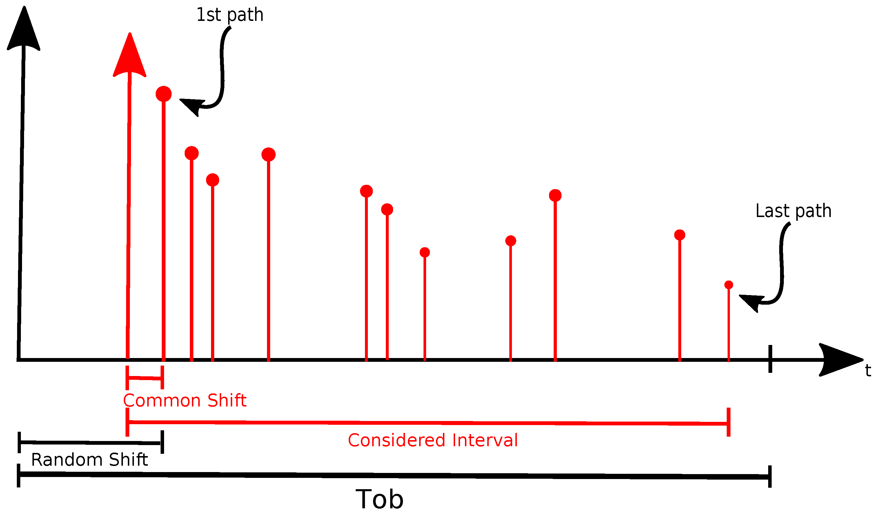
where, as widely accepted in the context of UWB indoor propagation, a clustered arrival of paths is assumed [27]. With reference to Equation (4), C indicates the total number of clusters of paths forming the CIR, and $R(c)$ indicates the number of paths composing the cth cluster; moreover, ${\tau }_{c,r}$ and $a_{c,r}$ indicate the time of arrival and the amplitude of the rth path within the cth cluster, respectively, and finally G indicates the total multipath gain, which measures the total amount of energy collected over all paths when a pulse with unitary energy is transmitted [28,29]. In the proposed scheme, the absence of perfect time synchronization is considered between both AN/RN and AN/AN pairs; for this reason, ${\tau }_{1,1}$ in Equation (4) does not correspond to the true ToA: in fact, the Tx signal is observed at each AN with a random initial shift, caused by the mismatch between the initial time of transmission and observation. In order to avoid the shift in the evaluation of ${\tau }_{\mathtt{rms}}$, CIRs for all ANs/RNs have been aligned to a common ${\tau }_{1,1}$ shift value, as shown in Figure 1.

With reference to the notation introduced in Section 4.1, UWB fingerprints ${\mathit{s}}_n$ and ${\mathit{t}}_m$ are thus defined as ${\mathit{s}}_n=\{{\mathit{s}}_n^1,{\mathit{s}}_n^2\}$ and ${\mathit{t}}_m=\{{\mathit{t}}_m^1,{\mathit{t}}_m^2\}$, respectively.

The components ${\mathit{s}}_n^1$ and ${\mathit{t}}_m^1$ of fingerprints are based on the first CIR feature identified above and thus contain the set of energy values for each AN/RN and AN/TN pair. Denoting as ${\mathcal{E}}^{n,l}$ the energy for the pair formed by the nth RN and the lth AN, it follows that ${\mathit{s}}_n^1=({\mathcal{E}}^{n,1},\cdots ,{\mathcal{E}}^{n,L_j})$ and ${\mathit{t}}_m^1=({\mathcal{E}}^{m,1},\cdots ,{\mathcal{E}}^{m,L_j})$; similarly, components ${\mathit{s}}_n^2$ and ${\mathit{t}}_m^2$ of the fingerprints are based on the second CIR feature and thus include the set of RMS-DS values for each AN/RN and AN/TN pair. Denoting as ${\tau }_{\mathtt{rms}}^{n,l}$ the RMS-DS for the pair formed by the nth RN and the lth AN, it follows that ${\mathit{s}}_n^2=({\tau }_{\mathtt{rms}}^{n,1},\cdots ,{\tau }_{\mathtt{rms}}^{n,L_j})$ and similarly ${\mathit{t}}_m^2=({\tau }_{\mathtt{rms}}^{m,1},\cdots ,{\tau }_{\mathtt{rms}}^{m,L_j})$.

4.3. Algorithms

Two algorithms are considered for position estimation: the first, fixed kNN, is taken from the literature, while the second, adaptive kNN, is newly introduced in this work.

Fixed kNN—Following the traditional approach adopted in most fingerprinting systems, the algorithm adopts as the similarity metric the inverse Euclidean distance between two fingerprints, corresponding to the inverse of the Minkowski distance defined in Equation (2) with order $o=2$, in combination with a fixed k.

Adaptive kNN—The algorithm adapts the value of k on the basis of the fingerprint collected at the position of the TN by also taking advantage of multifeature fingerprints, when available. The algorithm is organized into $F+1$ steps and uses an iterative approach that eventually selects fingerprints for which all features meet a similarity condition defined on the basis of dynamic thresholds. In the following, the algorithm is described for the case of multifeature UWB fingerprints with $F=2$, while its application to monofeature WiFi fingerprints is presented at the end of the section.

• (a)

  For each generic nth RN, given ${\mathit{s}}_n^1$ and ${\mathit{t}}_m^1$, a vector ${\mathit{\alpha }}_{n,m}^1=({\alpha }_{n,m,1}^1,\cdots ,{\alpha }_{n,m,L_j}^1)$ is defined, where the generic lth component is defined as follows:

  $${\alpha }_{n,m,l}^1=\left\{\begin{array}{c}\hfill \frac{{\mathcal{E}}^{m,l}}{{\mathcal{E}}^{n,l}}\mathrm{if}{\mathcal{E}}^{m,l}>{\mathcal{E}}^{n,l}\\ \hfill \frac{{\mathcal{E}}^{n,l}}{{\mathcal{E}}^{m,l}}\mathrm{if}{\mathcal{E}}^{n,l}>{\mathcal{E}}^{m,l}\end{array}\right.$$

  Each component of ${\mathit{\alpha }}_{n,m}^1$ is by definition $\ge 1$ and defines a similarity metric for the lth component of fingerprints ${\mathit{s}}_n^1$ and ${\mathit{t}}_m^1$: ${\alpha }_{n,m,l}^1\to 1$ means that, with reference to the lth AN, the nth RN experiences an energy similar to that of the TN, thus possibly corresponding to similar positions in the area.

  (b)

  A set of thresholds ${\{\delta \}}^1=\{{\delta }_{min}^1,\cdots ,{\delta }_i^1,\cdots ,{\delta }_{max}^1\}$ is defined in order to assess whether ${\mathit{s}}_n^1$ and ${\mathit{t}}_m^1$ are similar, on the basis of ${\mathit{\alpha }}_{n,m}^1$. For the generic ith threshold ${\delta }_i^1$ selected from ${\{\delta \}}^1$, the lth components of ${\mathit{s}}_n^1$ and ${\mathit{t}}_m^1$ are considered similar if ${\alpha }_{n,m,l}^1\le {\delta }_i^1$. In turn, ${\mathit{s}}_n^1$ and ${\mathit{t}}_m^1$ are determined as similar if at least $\lceil L_j/2\rceil$ components have been considered similar. Thresholds are selected one by one, starting from the most restrictive, ${\delta }_{min}^1$, and the similarity of each RN to the TN is tested against it. When at least one RN is determined to be similar to the TN, the procedure is concluded.

  The RNs passing the selection of steps 1a and 1b are considered similar to the TN in the energy domain, and they are transferred to step 2.
• The same procedure defined in steps 1a and 1b for the energy domain is applied in the RMS-DS domain by defining the ${\mathit{\alpha }}_{n,m}^2$ vectors on the basis of ${\mathit{s}}_n^2$ and ${\mathit{t}}_m^2$ and by comparing their components with thresholds in a set ${\{\delta \}}^2=\{{\delta }_{min}^2,\cdots ,{\delta }_{max}^2\}$, leading to further pruning of the set of RNs eventually transferred to step 3.
• Equation (1) is finally applied on the set of remaining RNs in order to estimate the position of the TN.

The application of the algorithm to WiFi fingerprints as defined in Section 4.2 is straightforward and foresees a first step in which RSS values stored in fingerprints are used to define vectors ${\mathit{\alpha }}_{n,m}^1$ and prune the set of fingerprints as described in step 1 above, as well as a second step corresponding to step 3 above.

5. A Common Framework for Performance Comparison

This section provides details on the common framework used to compare the two systems.

The second floor of the Department of Information Engineering, Electronics and Telecommunications (DIET) of Sapienza University of Rome, Rome, Italy, covering a total area of approximately $42\times 12$ ${\mathrm{m}}^2$, was used as a testing area $\mathcal{A}$. Within $\mathcal{A}$, WiFi indoor propagation, and thus RSS values, were modeled by using the multi-wall multi-floor (MWMF) empirical model [30], with site-specific propagation parameters obtained with the methodology reported in [31,32]. In the case of UWB propagation, CIRs were modeled according to the IEEE 802.15.3a model [33].

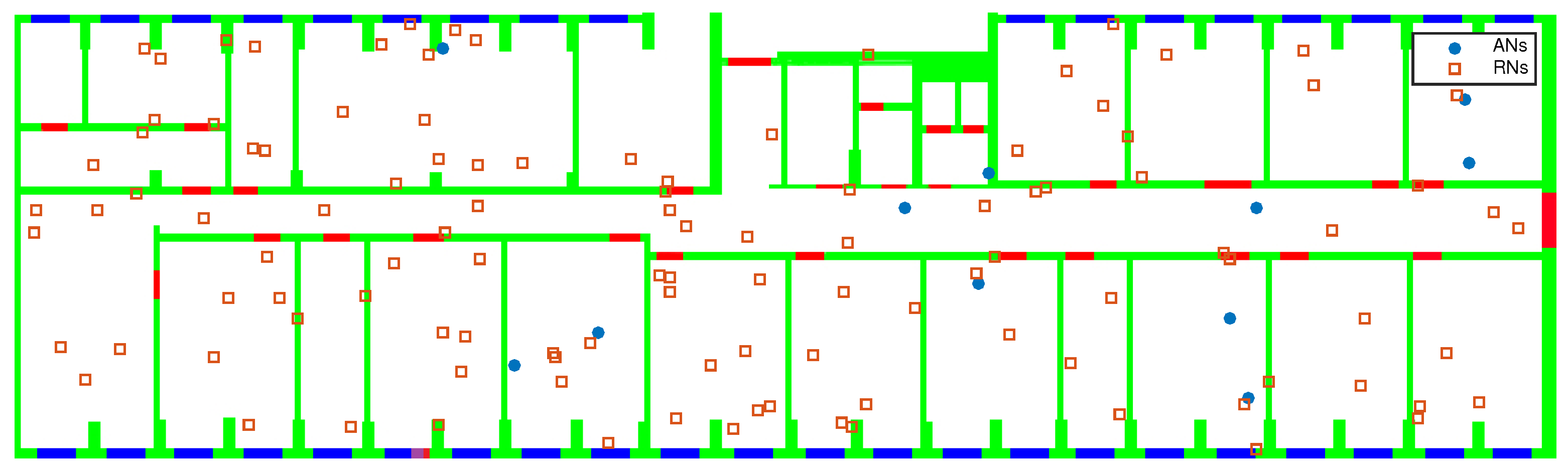
In order to derive general results, not strictly depending on a given AN/RN topology, independent PPPs were adopted in order to randomly select AN/RN positions and cardinalities. The performance results in terms of estimation accuracy were then averaged over 100 topologies. Given the general relationship $\overline{N}=\lambda \left|\mathcal{A}\right|$, density values, denoted as ${\lambda }_{\mathtt{AN}}$ and ${\lambda }_{\mathtt{RN}}$, were selected in order to obtain, for each scenario, a realistic average number of ANs/RNs, denoted as $\overline{L}$ and $\overline{N}$, respectively. Figure 2 reports an example of AN/RN topology. For each topology, after defining a total number M of randomly distributed TNs, the positioning error ${ϵ}_m$ (with $m=1,2,\cdots ,M$) was evaluated for each TN as follows:

$${ϵ}_m=\sqrt{{(x_m^{\ast }-{\widehat{x}}_m)}^2+{(y_m^{\ast }-{\widehat{y}}_m)}^2+{(z_m^{\ast }-{\widehat{z}}_m)}^2}$$

(5)

where ${\widehat{\mathit{p}}}_m=({\widehat{x}}_m,{\widehat{y}}_m,{\widehat{z}}_m)$ and ${\mathit{p}}_m^{\ast }=(x_m^{\ast },y_m^{\ast },z_m^{\ast })$ are the estimated position and the true position for the mth TN, respectively. Assuming each ${ϵ}_m$ as a sample of a random variable $ϵ$, the cumulative distribution function (CDF) and the main statistics of $ϵ$, together with the average error $\overline{ϵ}=\frac{{\sum }_{m=1}^M{ϵ}_m}{M}$, were also evaluated.

6. Results and Discussions

In this section, the main results of the comparative analysis between the WiFi- and UWB-based fingerprinting are presented. Positioning errors ${ϵ}_m$ have been evaluated by using the simulation parameters reported in

Table 1. Simulation parameters.

Parameter	WiFi/UWB
M	50
$\overline{L}$	$\{5,10,15\}$
$\overline{N}$	$\{25,50,100\}$
k (fixed kNN)	$\{1,2,3,4,5\}$
${\{\delta \}}^{1,2}$ (adaptive kNN)	{1.1–1.5}

; among several possible combinations, three different ANs/RNs density scenarios were used for the initial performance comparison, referred to as low, medium and high density (LD, MD, and HD, respectively), as reported in

Table 2. ANs/RNs density scenarios.

Scenario	($\overline{\mathit{L}}$,$\overline{\mathit{N}}$)
Low density (LD)	($5,25$)
Medium density (MD)	($10,50$)
High density (HD)	($15,100$)

. We note that in the following, error statistics are summarized in the form of boxplot diagrams, in which the reported statistics are minimum, maximum, and median errors, and 25th and 75th percentiles. Diagrams also report possible outliers, evaluated as a function of the values found for the 25th/75th percentiles and their difference to minimum and maximum errors, respectively. In particular, a value is considered an outlier if it is smaller than $q_{25\%}-\mathrm{\Delta }(q_{75\%}-q_{25\%})$ or larger than $q_{75\%}+\mathrm{\Delta }(q_{75\%}-q_{25\%})$, where $q_{25\%}$ and $q_{75\%}$ represent the 25th/75th percentiles, respectively, and $\mathrm{\Delta }$ is the greatest value between the difference evaluated among the 75th percentile and the maximum error and the difference between the 25th percentile and the minimum error.

6.1. Fixed kNN

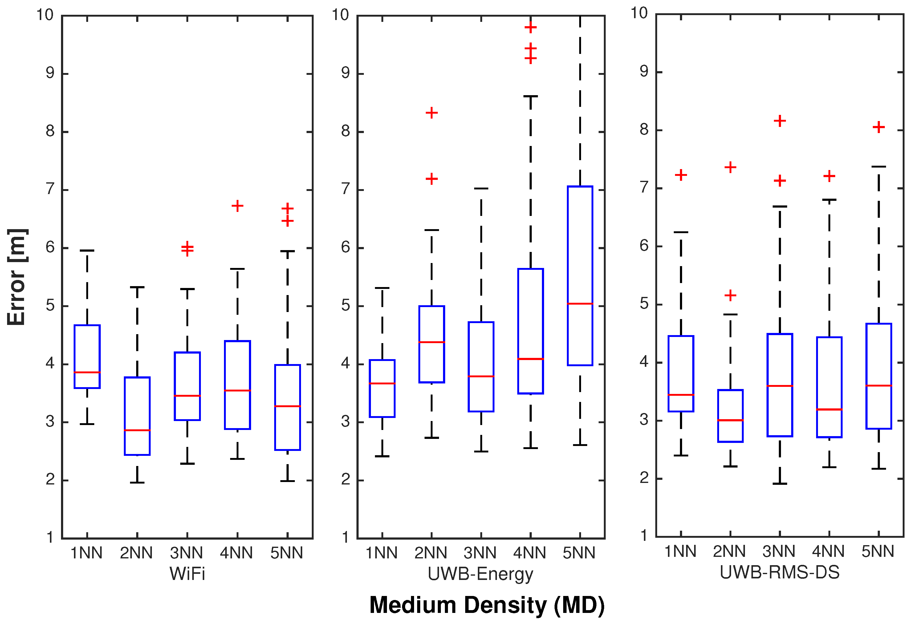
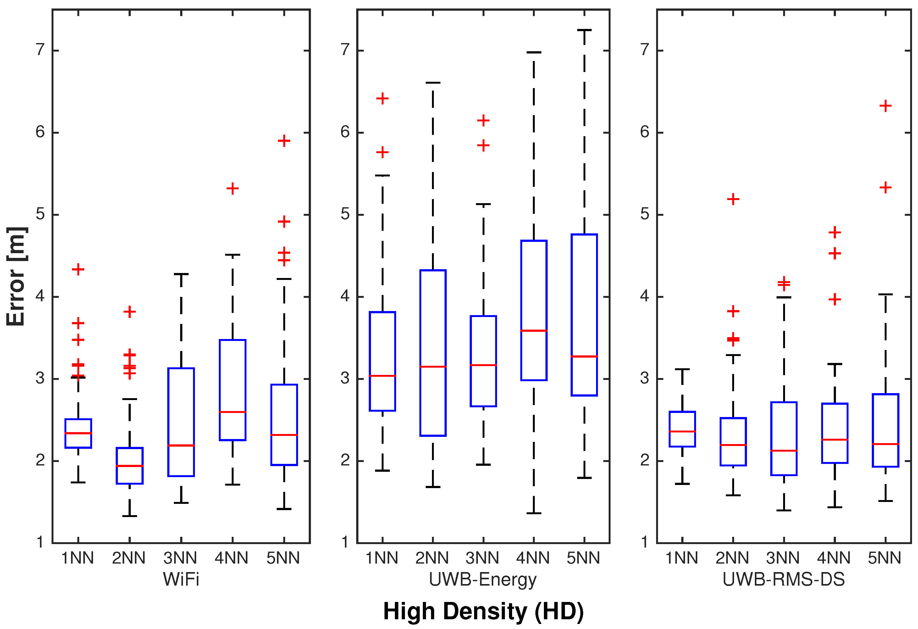
Because the fixed kNN algorithm does not support the use of multifeature fingerprints, in the analysis presented in this subsection, WiFi was compared with UWB using either of the two features, leading to three different systems: (a) WiFi; (b) UWB-energy, only using CIR energy; and (c) UWB-RMS-DS, only using CIR RMS-DS. Figure 3, Figure 4 and Figure 5 report statistics of $ϵ$ for the three systems, for k ranging from 1 to 5, in LD, MD, and HD scenarios, respectively.

The results highlight that, as expected, the positioning accuracy of all systems increases as the densities of both the ANs and RNs increase. Notably, a slightly better performance of WiFi RSS with respect to UWB-energy could be observed, with the gap in favor of WiFi increasing as the ANs/RNs densities increased. This could be explained by observing that the RSS values generated by the deterministic MWMF model used for WiFi were characterized by a lower variability compared to the energy values obtained from UWB CIRs generated with the statistical IEEE 802.15.3a channel model. The validity of the MWMF model in generating WiFi RSS fingerprints was assessed in [32,34].

Moving to the comparison of WiFi versus UWB-RMS-DS, the results show a similar performance for the two systems, highlighting a high reliability of the RMS-DS feature in representing the UWB CIR.

Finally, the results show that the setting $k=2$ leads to the best performance for WiFi in terms of median error in all density scenarios.

6.2. Adaptive kNN

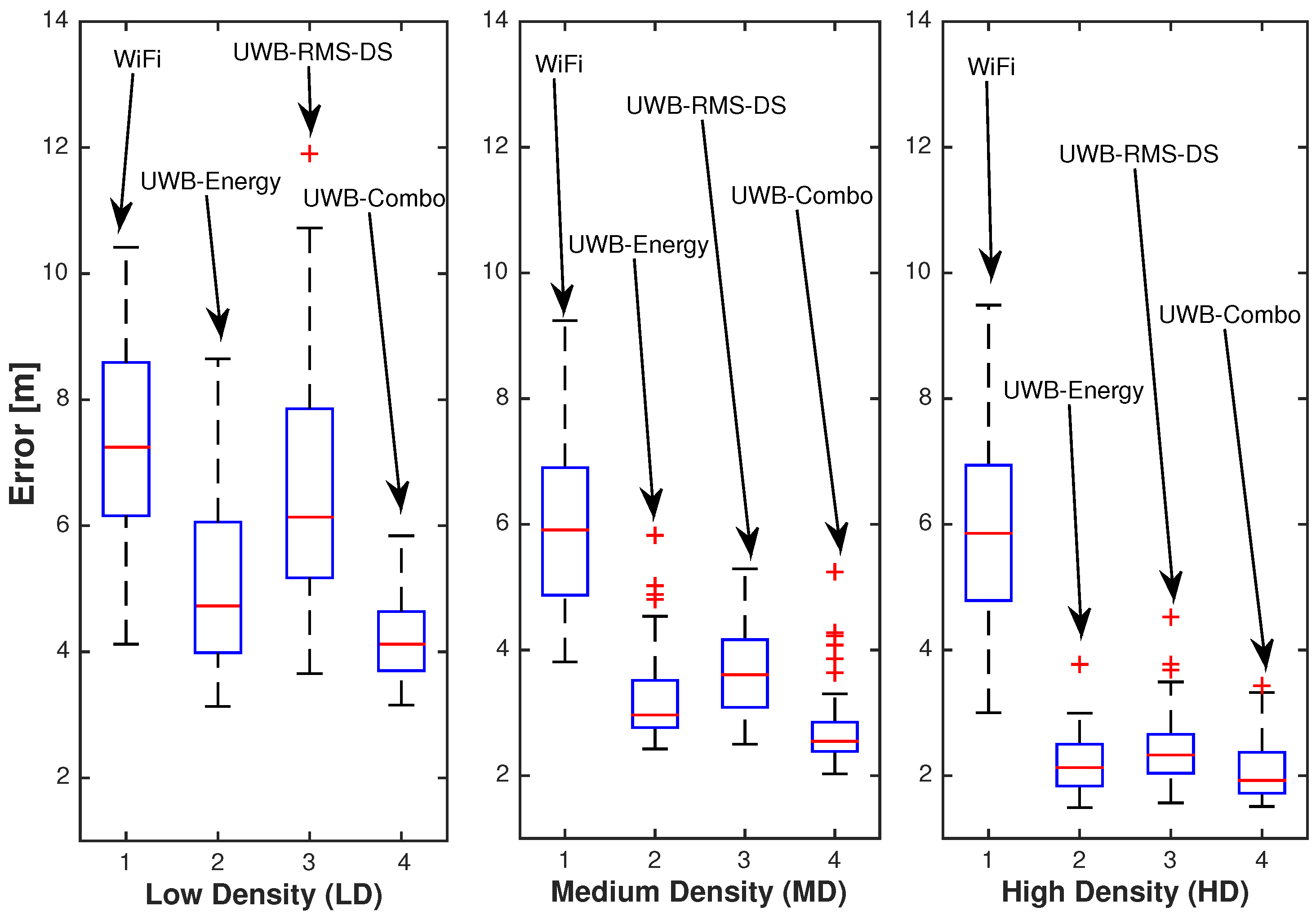
The adaptive kNN algorithm introduced in this work can take advantage of the multifeature UWB fingerprints; out of completeness, however, the analysis presented in this subsection also considers the two UWB systems introduced in Section 6.1. As a result, Figure 6 reports statistics of $ϵ$ in LD, MD, and HD scenarios for the WiFi RSS system versus three different UWB IPSs: UWB-energy and UWB-RMS-DS previously introduced, as well as the UWB-combo system, using both UWB CIR features.

Several insights can be obtained from the results shown in Figure 6. In particular, a significant decrease in accuracy for the WiFi system compared to that achieved with the fixed kNN algorithm can be observed; oppositely, a significant accuracy increase is visible for both the UWB-energy and UWB-RMS-DS systems. The results thus indicate that the proposed algorithm is particularly suited for operating on UWB CIR features and peculiar propagation characteristics.

The results also show that the UWB-combo system outperforms WiFi and both UWB systems on the basis of stand-alone CIR features, indicating that the proposed algorithm is effective in taking advantage of multifeature fingerprints.

6.3. UWB versus WiFi-Optimal Configuration

The results in Section 6.1 and Section 6.2 highlight that the two algorithms lead to significantly different performances when applied to WiFi versus UWB technologies. This section compares the two technologies when each is used in combination with the algorithm leading to the best possible performance; in particular, the fixed kNN algorithm with $k=2$ was selected for WiFi (configuration referred to as WiFi-opt in the following) and the UWB-combo scheme introduced in Section 6.2 was considered for UWB. The impact of ANs/RNs densities, topologies, and procedures for system optimization of the two technologies is analyzed in the following; finally, the computational complexity characterizing the two schemes is discussed.

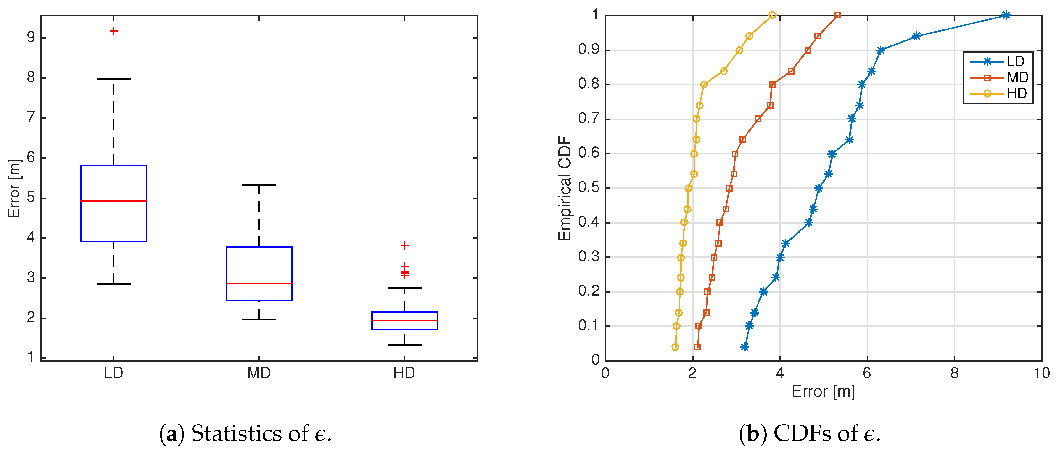
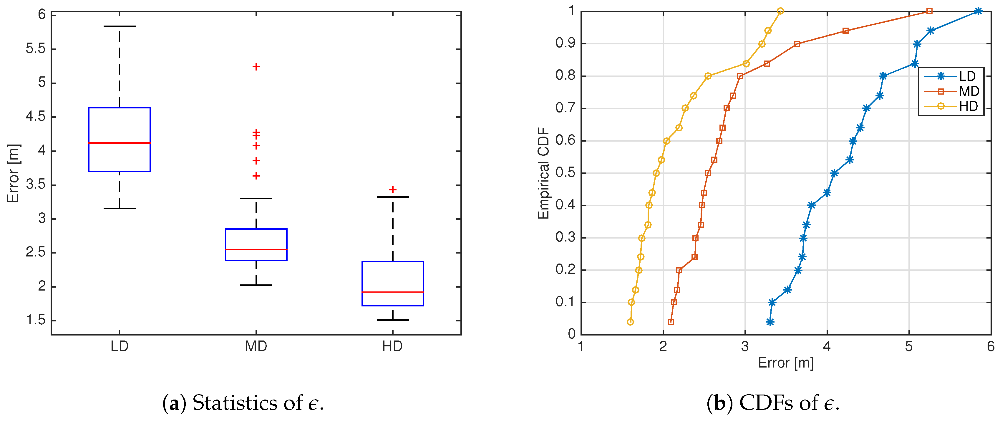
Impact of ANs/RNs Densities—Figure 7 and Figure 8 report the statistics and CDF of $ϵ$ in the LD, MD and HD scenarios for WiFi-opt and UWB-combo, respectively. The results show that UWB-combo outperforms WiFi-opt in all density scenarios, always showing a lower median $ϵ$ than WiFi; UWB-combo and WiFi-opt present some outliers in the MD and HD scenarios, respectively, ranging however on tight intervals close to the median error.

Interestingly, the results show that when the two technologies are compared under fair conditions, the performance advantage of UWB, although still significant, is not as wide as the results in [12,13,14] might suggest.

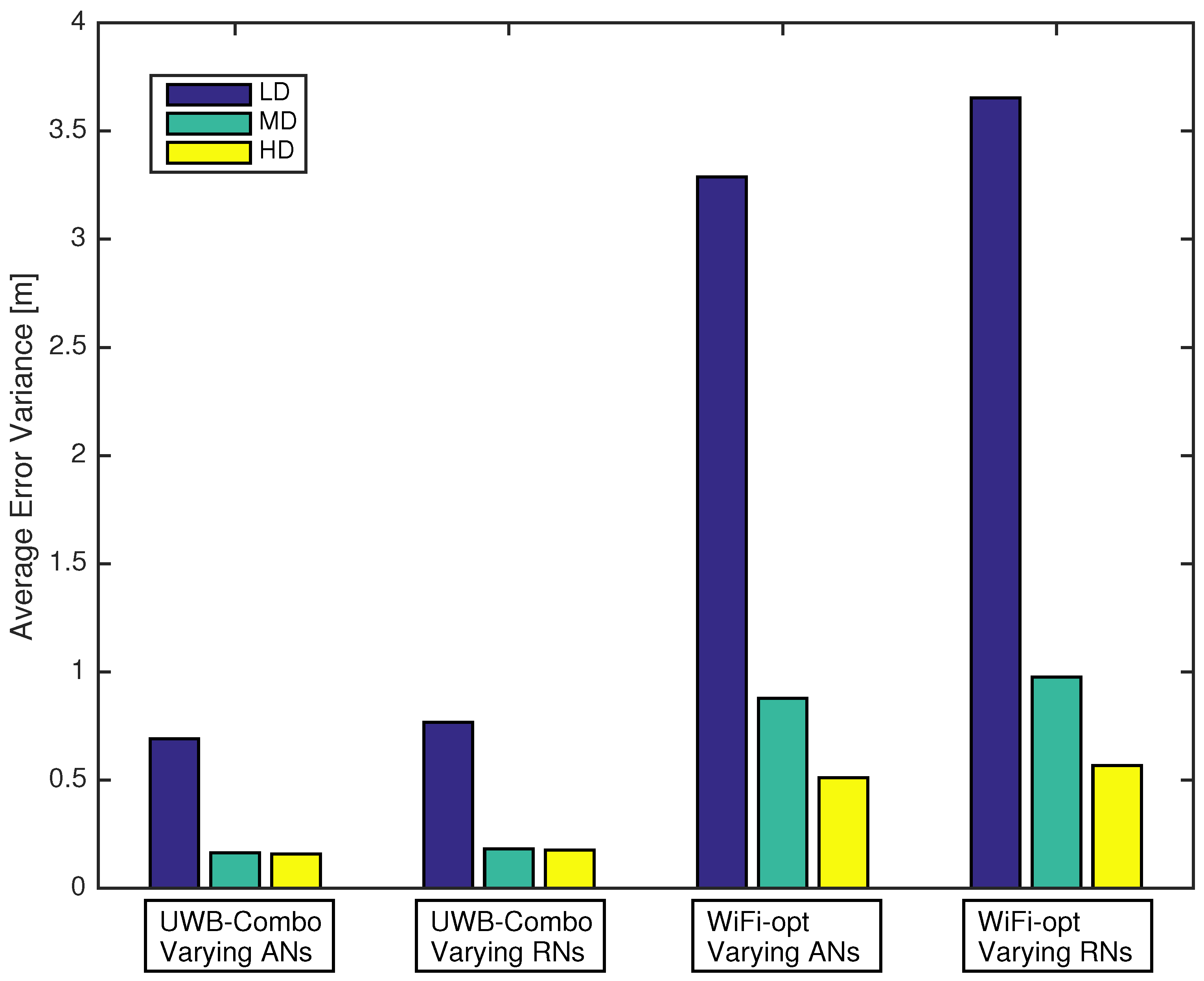
Impact of ANs/RNs Topologies—Previous results have been obtained by averaging the positioning errors of different ANs/RNs topologies. In order to highlight how the variability related to ANs/RNs topology affects the positioning accuracy and reliability, Figure 9 shows, for all density scenarios defined in Table 2, the variance of the average error $\overline{ϵ}$ when (1) the ANs topologies change while the RNs topology is fixed, and (2) the RNs topologies change while the ANs topology is fixed. The results show that, for both systems, the variation of either the ANs or RNs topology has a similar impact on the positioning error. However, a significantly higher impact is observed for WiFi-opt, indicating that UWB-combo not only outperforms WiFi-opt in terms of accuracy, but its performance is also less affected by the variation of ANs/RNs placement, allowing a higher degree of freedom in system implementation.

Impact of System Optimization—The two systems were further compared in terms of robustness with respect to system optimization. On the one hand, the optimization may focus on the reduction of the dedicated infrastructure in terms of the number of ANs; on the other, it may focus on the reduction of required offline measurements in terms of the number of RNs. Two additional scenarios were thus defined, as reported in

Table 3. ANs/RNs optimized scenarios.

Scenario	$\overline{\mathit{L}}$	$\overline{\mathit{N}}$
Minimum infrastructure (mI)	5	$\{25,50,100\}$
Minimum measurements (mM)	$\{5,10,15\}$	25

.

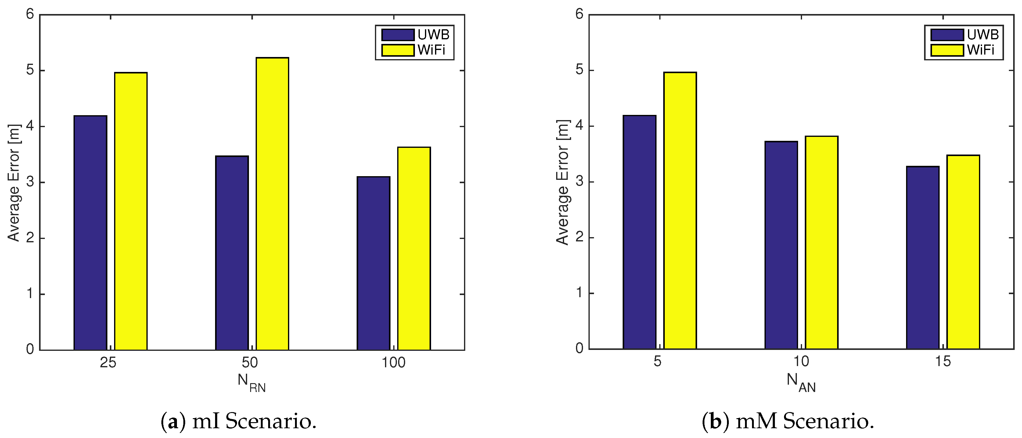
Figure 10 reports the average positioning error for WiFi-opt versus UWB-combo in minimum infrastructure (mI) and minimum measurements (mM) scenarios, respectively. The results show that also in this case UWB-combo outperforms WiFi-opt in terms of the average positioning error in both the mI and mM scenarios, opening the way to more-efficient optimization procedures in terms of the density of both ANs and RNs.

Complexity Comparison—The comparison between the complexity of WiFi-opt and UWB-combo should consider both offline and online phases for the two systems:

• Offline-phase complexity—The complexity of the measurement phase is comparable for the two systems: in the case of WiFi-opt, the RSS reading taken at each RN is commonly provided by off-the-shelf WiFi devices and does not require any particular advanced post-processing. Similarly, energy and RMS-DS readings, taken in the same number of RNs, can be easily obtained from data collected by off-the-shelf UWB devices, such as Decawave or Time Domain products, with simple post-processing techniques [35]. In terms of fingerprinting database storage, the UWB-combo needs twice the storage space compared to WiFi-opt, as two signal features are included in the fingerprint associated to a single RN. However, the results shown in Figure 10 indicate that UWB-combo can achieve the same positioning accuracy while using a lower RN density than WiFi-opt, in turn requiring less storage space.
• Online-phase complexity—The complexity of this phase depends on the adopted estimation algorithm.
  In the case of WiFi-opt, a traditional kNN algorithm is used; following the analysis presented in [36], the kNN complexity is determined by the computation of the Euclidean distances between TN and RNs RSS fingerprints ($\overline{N}\overline{L}$ multiplications) and the selection of the k nearest neighbors ($\overline{N}k$ comparisons). Overall, the asymptotic complexity can be expressed as $O(\overline{N}\overline{L})$ in terms of multiplications and $O(\overline{N})$ in terms of comparisons.
  In the case of UWB-combo, the complexity of the adaptive kNN algorithm operating on $F=2$ features can be estimated as follows. In step 1, $\overline{N}\overline{L}$ values of ${\alpha }^1$ are computed ($\overline{N}\overline{L}$ multiplications) and compared with the set of ${\{\delta \}}^1$ thresholds. In the worst case, this comparison is repeated over the entire set of thresholds, leading to the need for $\overline{N}\overline{L}\left|{\{\delta \}}^1\right|$ comparisons, where ${|\{\delta \}}^1|$ represents the cardinality of the set of energy thresholds. In step 2, if no RNs have been discarded during step 1 (worst-case analysis), $\overline{N}\overline{L}$ values of ${\alpha }^2$ are computed ($\overline{N}\overline{L}$ multiplications) and compared with the set of ${\{\delta \}}^2$ thresholds. If this comparison is repeated over the entire set of thresholds, $\overline{N}\overline{L}\left|{\{\delta \}}^2\right|$ comparisons are needed, where ${|\{\delta \}}^2|$ represents the cardinality of the set of RMS-DS thresholds. The asymptotic complexity can finally be expressed as $O(\overline{N}\overline{L})$ in terms of multiplications and $O(\overline{N}\overline{L})$ in terms of comparisons.
  UWB-combo is thus characterized by a slightly higher asymptotic complexity than WiFi-opt, but it is worth mentioning that the above analysis was carried out under an extreme worst-case scenario, in which, in particular, it is assumed that step 1 of the algorithm does not affect the following phase (no RNs are discarded using the energy parameter). However, experimental analysis has showed that such a scenario is quite unlikely: most of the RNs are in fact typically discarded in step 1, leading to a significantly reduced complexity for latter phases of the algorithm.

7. Conclusions and Future Work

In this work, a comparison of WiFi- and UWB-based fingerprinting IPSs was carried out, in order to verify whether UWB technology can still lead to a higher accuracy with respect to WiFi when operating in scenarios characterized by the same AN and RN densities. The two technologies were compared using two different positioning algorithms: a traditional kNN algorithm with fixed k, and a novel adaptive kNN algorithm with dynamic k, designed in order to take advantage of fingerprints including multiple features, as typically made available by UWB hardware.

The results highlight that, when operating in combination with a traditional kNN algorithm with fixed k, UWB and WiFi technologies lead to similar accuracy, and that RMS-DS should be the preferred choice when only one feature can be used to represent UWB CIRs.

When used in combination with the proposed adaptive kNN algorithm, however, UWB leads to a higher accuracy and better robustness, in particular when resources, defined in terms of dedicated infrastructure and collected measurements, are minimized. Moreover, the analysis of average error variance shows that UWB is more robust than WiFi to variations in the topology of ANs and RNs, thus leading to a more stable positioning performance with respect to spatial variations of both the density and positions of ANs and RNs and thus supporting a simpler and faster implementation.

Future work will focus on extending the presented analysis by introducing performance comparison with traditional ToA-based UWB IPSs. Experimental measurements will also be introduced in the analysis in order to confirm the results obtained by simulation in this work, taking into account in particular the impact of varying environmental conditions over time on the IPS performance.

References

- Celebi, H.; Guvenc, I.; Gezici, S.; Arslan, H. Cognitive-Radio Systems for Spectrum, Location, and Environmental Awareness. IEEE Antennas Propag. Mag. 2010, 52, 41–61. [Google Scholar] [CrossRef]
- Macagnano, D.; Destino, G.; Abreu, G. Indoor positioning: A key enabling technology for IoT applications. In Proceedings of the IEEE World Forum on Internet of Things (WF-IoT), Seoul, Korea, 6–8 March 2014; pp. 117–118. [Google Scholar]
- Liu, H.; Darabi, H.; Banerjee, P.; Liu, J. Survey of Wireless Indoor Positioning Techniques and Systems. IEEE Trans. Syst. Man Cybern. Part C (Appl. Rev.) 2007, 37, 1067–1080. [Google Scholar] [CrossRef]
- Gezici, S.; Zhi, T.; Giannakis, G.; Kobayashi, H.; Molisch, A.; Poor, H.V.; Sahinoglu, Z. Localization via ultra-wideband radios: A look at positioning aspects for future sensor networks. IEEE Signal Process. Mag. 2005, 22, 70–84. [Google Scholar] [CrossRef]
- Honkavirta, V.; Perala, T.; Ali-Loytty, S.; Piche, R. A comparative survey of WLAN location fingerprinting methods. In Proceedings of the 6th Workshop on Positioning, Navigation and Communication (WPNC), Leibniz, Hannover, Germany, 19 March 2009; pp. 234–251. [Google Scholar]
- Dardari, D.; Conti, A.; Ferner, U.; Giorgetti, A.; Win, M.Z. Ranging With Ultrawide Bandwidth Signals in Multipath Environments. Proc. IEEE 2009, 97, 404–426. [Google Scholar] [CrossRef]
- Guvenc, I.; Chong, C.C. A Survey on TOA Based Wireless Localization and NLOS Mitigation Techniques. IEEE Commun. Surv. Tutor. 2009, 11, 107–124. [Google Scholar] [CrossRef]
- Althaus, F.; Troesch, F.; Wittneben, A. UWB geo-regioning in rich multipath environment. In Proceedings of the IEEE 62nd Vehicular Technology Conference—Fall, Dallas, TX, USA, 28 September 2005; pp. 1001–1005. [Google Scholar]
- Steiner, C.; Althaus, F.; Troesch, F.; Wittneben, A. Ultra-wideband geo-regioning: A novel clustering and localization technique. EURASIP J. Adv. Signal Process. 2008, 2008, 1–13. [Google Scholar] [CrossRef]
- Steiner, C.; Wittneben, A. Low Complexity Location Fingerprinting with Generalized UWB Energy Detection Receivers. IEEE Trans. Signal Process. 2010, 58, 1756–1767. [Google Scholar] [CrossRef]
- Kroll, H.; Steiner, C. Indoor ultra-wideband location fingerprinting. In Proceedings of the International Conference on Indoor Positioning and Indoor Navigation (IPIN), Zurich, Switzerland, 15–17 September 2010; pp. 1–5. [Google Scholar]
- Taok, A.; Kandil, N.; Affes, S.; Georges, S. Fingerprinting Localization Using Ultra-Wideband and Neural Networks. In Proceedings of the International Symposium on Signals, Systems and Electronics, Montreal, QC, Canada, 30 July–2 August 2007; pp. 529–532. [Google Scholar]
- Yu, L.; Laaraiedh, M.; Avrillon, S.; Uguen, B. Fingerprinting localization based on neural networks and ultra-wideband signals. In Proceedings of the IEEE International Symposium on Signal Processing and Information Technology (ISSPIT), Bilbao, Spain, 14–17 December 2011. [Google Scholar]
- Luo, J.; Huanbin, G. Deep Belief Networks for Fingerprinting Indoor Localization Using Ultrawideband Technology. Int. J. Distrib. Sens. Netw. 2016, 12, 1–8. [Google Scholar] [CrossRef]
- Win, M.Z.; Scholtz, R.A. On the robustness of ultra-wide bandwidth signals in dense multipath environments. IEEE Commun. Lett. 1998, 2, 51–53. [Google Scholar] [CrossRef]
- Bahl, P.; Padmanabhan, V.N. RADAR: An in-building RF-based user location and tracking system. In Proceedings of the 19th Annual Joint Conference of the IEEE Computer and Communications Societies (INFOCOM), Tel Aviv, Israel, 26–30 March 2000; pp. 775–784. [Google Scholar]
- Li, B.; Salter, J.; Dempster, A.G.; Rizos, C. Indoor positioning techniques based on wireless LAN. In Proceedings of the 1st IEEE International Conference on Wireless Broadband and Ultra Wideband Communications, Sydney, Australia, 24–27 September 2006; pp. 13–16. [Google Scholar]
- Yu, F.; Jiang, M.; Liang, J.; Qin, X.; Hu, M.; Peng, T.; Hu, X. 5G WiFi Signal-Based Indoor Localization System Using Cluster k-Nearest Neighbor Algorithm. Int. J. Distrib. Sens. Netw. 2014, 10, 1–12. [Google Scholar] [CrossRef]
- Caso, G.; de Nardis, L.; di Benedetto, M.G. Frequentist inference for WiFi fingerprinting 3D indoor positioning. In Proceedings of the IEEE International Conference on Communication—Workshops, Beijing, China, 10–14 August 2015; pp. 809–814. [Google Scholar]
- Caso, G.; de Nardis, L.; di Benedetto, M.G. A Mixed Approach to Similarity Metric Selection in Affinity Propagation-Based WiFi Fingerprinting Indoor Positioning. Sensors 2015, 15, 27692–27720. [Google Scholar] [CrossRef] [PubMed] [Green Version]
- Lemic, F.; Handziski, V.; Caso, G.; de Nardis, L.; Wolisz, A. Enriched Training Database for improving the WiFi RSSI-based indoor fingerprinting performance. In Proceedings of the IEEE Annual Consumer Communications & Networking Conference (CCNC), Las Vegas, NV, USA, 6–13 January 2016; pp. 875–881. [Google Scholar]
- Cardinali, R.; de Nardis, L.; Lombardo, P.; di Benedetto, M.G. UWB Ranging accuracy in High- and Low-Data-Rate Applications. IEEE Trans. Microw. Theory Tech. 2006, 54, 1865–1875. [Google Scholar] [CrossRef]
- Shin, B.; Lee, J.; Lee, T.; Kim, H. Enhanced weighted K-nearest neighbor algorithm for indoor WiFi positioning systems. In Proceedings of the International Conference on Computing Technology and Information Management (ICCM’12), Seoul, South Korea, 24–26 April 2012; pp. 574–577. [Google Scholar]
- Philipp, M.; Kessel, M.; Werner, M. Dynamic nearest neighbors and online error estimation for SMARTPOS. Int. J. Adv. Internet Technol. 2013, 6, 1–11. [Google Scholar]
- Heidari, M.; Pahlavan, K. Identification of the absence of direct path in toa-based indoor localization systems. Int. J. Wirel. Inform. Netw. 2008, 15, 117–127. [Google Scholar] [CrossRef]
- Marano, S.; Gifford, W.M.; Wymeersch, H.; Win, M.Z. NLOS identification and mitigation for localization based on UWB experimental data. IEEE J. Sel. Areas Commun. 2010, 28. [Google Scholar] [CrossRef]
- Saleh, A.A.M.; Valenzuela, R. A Statistical Model for Indoor Multipath Propagation. IEEE J. Sel. Areas Commun. 1987, 5, 128–137. [Google Scholar] [CrossRef]
- Ghassemzadeh, S.S.; Greenstein, A.; Kavcic, A.; Sveinsson, T.; Tarokh, V. An empirical indoor path loss model for ultra-wideband channels. J. Commun. Netw. 2003, 5, 303–308. [Google Scholar] [CrossRef]
- Di Benedetto, M.G.; Giancola, G. Understanding Ultra Wide Band Radio Fundamentals; Prentice Hall: Upper Saddle River, NJ, USA, 2004. [Google Scholar]
- Borrelli, A.; Monti, C.; Vari, M.; Mazzenga, F. Channel models for IEEE 802.11b indoor system design. In Proceedings of the IEEE International Conference on Communications, Paris, France, 20–24 June 2004. [Google Scholar]
- Caso, G.; de Nardis, L. On the Applicability of Multi-Wall Multi-Floor Propagation Models to WiFi Fingerprinting Indoor Positioning. In Future Access Enablers for Ubiquitous and Intelligent Infrastructures, Proceedings of the First International Conference, FABULOUS 2015, Ohrid, Republic of Macedonia, 23–25 September 2015; Springer International Publishing AG: Cham, Switzerland; pp. 166–172.
- Caso, G.; de Nardis, L. Virtual and Oriented WiFi Fingerprinting Indoor Positioning based on Multi-Wall Multi-Floor Propagation Models. Mobile Netw. Appl. 2017, 22, 825–833. [Google Scholar] [CrossRef]
- Foerster, J.R.; Pendergrass, M.; Molisch, A.F. A channel model for ultrawideband indoor communication. In Proceedings of the International Symposium on Wireless Personal Multimedia Communication, Abano Terme, Padua, Italy, 12–15 September 2004. [Google Scholar]
- Caso, G.; Nardis, L.D.; Lemic, F.; Handziski, V.; Wolisz, A.; Benedetto, M.D. ViFi: Virtual Fingerprinting WiFi-based Indoor Positioning via Multi-Wall Multi-Floor Propagation Model. arXiv 2016, arXiv:1611.09335. [Google Scholar]
- Decawave DW1000 Datasheet. Available online: https://www.decawave.com/sites/default/files/resources/dw1000-datasheet-v2.13.pdf (accessed on 16 January 2018).
- Zuo, W.; Zhang, D.; Wang, K. On kernel difference-weighted k-nearest neighbor classification. Pattern Anal. Appl. 2008, 11, 247–257. [Google Scholar] [CrossRef]
Figure 1.
Example of time alignment for a generic channel impulse response (CIR).
Figure 2.
Example of anchor node/target node (AN/RN) Poisson point process (PPP) topology @ DIET Department; and (ANs: circles; RNs: squares).
Figure 3.
Statistics of positioning error in low density (LD) scenario for WiFi, ultra-wideband (UWB)-energy and UWB root-mean-square delay spread (RMS-DS) with fixed k-nearest neighbor (kNN) algorithm ().
Figure 4.
Statistics of positioning error in medium density (MD) scenario for WiFi, ultra-wideband (UWB)-energy and UWB root-mean-square delay spread (RMS-DS) with fixed k-nearest neighbor (kNN) algorithm ().
Figure 5.
Statistics of positioning error in high density (HD) scenario for WiFi, ultra-wideband (UWB)-energy and UWB root-mean-square delay spread (RMS-DS) with fixed k-nearest neighbor (kNN) algorithm ().
Figure 6.
Statistics of positioning error in low, medium and high density (LD, MD and HD) scenarios for WiFi, ultra-wideband (UWB)-energy, UWB root-mean-square delay spread (RMS-DS) and UWB-combo with adaptive k-nearest neighbor (kNN) algorithm.
Figure 7.
Statistics (a) and cumulative distribution functions (CDFs) (b) of the positioning error in low, medium and high density (LD, MD and HD) scenarios for the WiFi-opt system.
Figure 8.
Statistics (a) and cumulative density functions (CDFs) (b) of the positioning error in low, medium and high density (LD, MD and HD) scenarios for the ultra-wideband (UWB)-combo system.
Figure 9.
Variance of average positioning error due to topology change in low, medium and high density (LD, MD and HD) scenarios for ultra-wideband (UWB)-combo vs WiFi-opt.
Figure 10.
Average positioning error in minimum infrastructure (mI) (a) and minimum measurements (mM) (b) scenarios for ultra-wideband (UWB)-combo vs WiFi-opt.