Mitigating Wind Induced Noise in Outdoor Microphone Signals Using a Singular Spectral Subspace Method ^†

Abstract

Wind induced noise is one of the major concerns of outdoor acoustic signal acquisition. It affects many field measurement and audio recording scenarios. Filtering such noise is known to be difficult due to its broadband and time varying nature. In this paper, a new method to mitigate wind induced noise in microphone signals is developed. Instead of applying filtering techniques, wind induced noise is statistically separated from wanted signals in a singular spectral subspace. The paper is presented in the context of handling microphone signals acquired outdoor for acoustic sensing and environmental noise monitoring or soundscapes sampling. The method includes two complementary stages, namely decomposition and reconstruction. The first stage decomposes mixed signals in eigen-subspaces, selects and groups the principal components according to their contributions to wind noise and wanted signals in the singular spectrum domain. The second stage reconstructs the signals in the time domain, resulting in the separation of wind noise and wanted signals. Results show that microphone wind noise is separable in the singular spectrum domain evidenced by the weighted correlation. The new method might be generalized to other outdoor sound acquisition applications.

1. Introduction

Recent and rapidly increasing research activities in acoustic sensing technology and acoustic signals along with Internet of Things (IoT) motivated the use of sound signatures to identify objects, sense the environmental variables and capture relevant events. Sound signal acquisition is one of the key stages in acoustics and audio engineering.

In the literature, many state of the art techniques that based on acoustic signals have been applied in many applications [1]. Recently, acoustic signals are used in diagnostic techniques of machines in the field of industry and engineering, where many rotating machines such as electric motors are used. Diagnosis of such motors is considered as a normal maintenance process [1]. Using acoustic signals is nowadays an up-to-date method for many applications of fault diagnosis and localisation in rotating machines. For example, in [1,2], acoustic signals are used for early fault diagnosis of bearing and stator faults of single-phase induction motor. In [3], they are used for automatic bearing fault localisation. A pattern recognition system was proposed and developed based on acoustic signals for automatic damage detection on composite materials where Singular Value Decomposition (SVD) method was used to filter acoustic signals [4]. In [5], the authors provide analysis of using acoustic signal processing for the recognition of rotor damages in a DC motor. In practice, acoustic signals have been used in many cases for early diagnosis of electric motors such as rotor damages of three-phase induction motor and loaded case synchronous motor [6,7]. A description of monitoring acoustic emission-based condition is given in [8]. Online monitoring of machines allows for intelligent maintenance with the optimised usage of maintenance resources [1].

In work environment and industrial conditions where many machines are used, workers are exposed to noise levels that often exceed permissible values. At such workplaces, noise is defined as any undesirable sound that causes harmful or tiring to human health [9]. The measurement of noise becomes increasingly important in order to maintain noise levels under the permissible values. In [9], the authors applied their method for measuring noise in work environment based on the acoustic pressure of noise emitted by CNC machines. Using acoustic holography methods for identifying and monitoring of noise sources of CNC machine tools were presented in [10].

In most of the applications of fault diagnosis of the motors when using acoustic signals, the idea is based on using condenser microphone or a group of microphones simultaneously for audio signal acquisition considering many factors that affect the fault frequencies such as motor speed along with the interferences of the environmental noises as the acoustical approach is sensitive to such noises. Importantly, calculating the frequency spectra of acoustic signals of the rotating machine, applying feature extraction methods; such as correlation and wavelet transformation along with data classification methods are required for the complete procedure of fault diagnosis [1]. In this paper, we turn our attention to particularly focus on sound signal acquisition in outdoor conditions.

Outdoor acoustic sensing is particularly challenging, as the transducers, typically microphones, are exposed to adverse weather conditions such as rain and wind, which might induce extraordinary noises in microphone signals. In this paper, the terminology “microphone wind noise” and/or “wind noise in microphone signals” refers to such noise of concern induced by the presence of a microphone in windy conditions.

Environmental systems are often considered ill-structured domains and environmental data set is commonly noisy and skewed [11]. Therefore, it is indicted that before investigating the dataset of interest and applying a process of knowledge discovery in databases, another tool should be used to reduce the noise even though defining the noise component from such a noisy structure can be difficult [11]. The frequency spectrum of noise depends on specific environmental measurement and it is generally uncertain [12].

Wind induced noise in microphone signals represents a typical example of this. In environmental noise monitoring, environmental sounds are such a rich source of acoustic data and at the same time they comprise much background noise, which hinder the extraction of useful information [13]. Environmental sounds are underexploited source of data. The presence of noises such as wind noise masks acoustic data and limits the use of such data source to efficiently extract useful information. For environmental noise level measurement, especially long-term measurement or monitoring, microphone wind noise is added to the recorded noise level, giving inaccurate results. It is well known that residual microphone wind noise is problematic [14].

For outdoor sound source recognition and event detection, the performance of signal processing algorithms such as speech or speaker recognition and event sound detection is affected by the wind noise in general [15]. For example, outdoor acoustic sensing can be applied to collect information about environmental changes by analysing wild life activities such as birds’ calls [16]. Microphone wind noise is known to be a serious problem that affects the sensed data in such outdoor sound acquisition [17].

Turbulence due to high speed airflow interacting with the microphone casing and diaphragm inside the microphone is one of the major causes of the microphone wind noise, which is considered a particular type of acoustic interference that results in a relatively high noise level [15]. The fluctuations that occur naturally in the wind are the second major component of wind noise [15]. Wind noise fluctuates rapidly and wind gusts might have very high energy [18]. The spectrum of the recorded wind noise has been described as a broadband but decreasing function of frequency, showing the bulk of the energy in the lower region of the spectrum [15]. Wind noise is highly non-stationary in time and even sometimes it resembles transient noise which makes it hard for an algorithm to estimate the noise from a noisy signal [18].

To deal with microphone wind noises, a large number of standard or common approaches ranging from fixed, optimal to adaptive filtering have been proposed in the past [18]. These methods worked to some extent but have intrinsic limitations of distorting wanted signals, high and varying residual wind noise and difficulties in retaining accurate signal energy levels to meet the measurement and analysis requirements. For event detection or decision making from acoustic signatures, distorted signals cause errors or misjudgements, mitigating the reliability, usability or even safety of such systems [19]. Existing noise reduction schemes, such as spectral subtraction or statistical-based estimators, cannot effectively attenuate wind noise [20]. Multi-microphone and microphone array are considered relatively effective for reducing wind noise as the difference in propagation delay between wind and acoustic waves can be exploited [15]. However, the difficulties and restrictions in setting up large arrays outdoor and high cost in deploying arrays limit their prevalent use. Single-microphone wind-noise reduction is still an open-ended research question and a technical challenge for further extensive study.

Contemporary and powerful signal processing methods are sought to address the wind noise issues which might yield better results, (e.g., [18]). Linear separation in subspace seems to be a potential solution to circumvent various aforementioned problems. For example, it has been successfully implemented for extracting trends from acoustic signals without any restriction on the length of the analysed time record [21].

This paper presents a new approach to wind noise reduction. Instead of filtering, a separation technique is developed. Signals are separated into wanted sounds of specific interest and wind noise, with reduced distortion imposed on the wanted signals, based on the statistical feature of wind noise. The new technique is based on the Singular Spectrum Analysis (SSA) method. Most recently the use of the SSA to address the wind noise reduction has been explored by the authors in a pilot study [22]. This paper further develops the work to give a complete treatment of the method taking into account the separation capability assessment. This paper explores the potentials and effectiveness of this method in wind noise separation and reduction. To the best of the authors’ knowledge, this represents the first attempt to handle microphone wind noise with singular spectrum analysis.

Following a brief justification of selecting the SSA method, this paper discusses the potentials of the SSA for microphone wind noise reduction, outlines its theory, methodology and mathematical formulation, presents the algorithm and some experimental results and provides analysis and discussion.

2. Rationale

As the SSA method decomposes a time series into its singular spectral domain components, which are physically meaningful in terms of oscillatory components and trends and reconstructs the series by leaving the random noise component behind, such fundamentals give it a great advantage for noise reduction [23,24,25]. Furthermore and unlike many other methods, the SSA works well even for small sample sizes making it possible to quickly update the coordinator rotation to varying signals block by block in relatively small blocks [26,27,28].

The SSA is generally applicable for many practical problems such as the study of classical time series, dynamical systems and signal processing along with multivariate statistics and multivariate geometry [23,29,30]. It is also an effective method for extraction of seasonality components, extraction of periodicities with varying amplitudes, finding trends of different resolution, smoothing, simultaneous extraction of complex trends and periodicities, finding structure in short time series, etc. The basic capabilities of the SSA can lead to solve all these problems [21,27,30,31,32].

A great deal of research work has been conducted on the SSA to consider it as a de-noising method [24,25,33]. The SSA technique has also been applied for extracting information from noisy dataset for biomedical engineering and other applications [34]. It has been recently seen many successful paradigms in the separation of biomedical signals, e.g., separating heart sound from lung noise and many other applications [34] and extracting the rhythms of the brain of electroencephalography [35]. The method has been employed and shown its capabilities for noise reduction for longitudinal measurements and surface roughness monitoring [26,30]. It has also been implemented for structural damage detection [36]. The superiority of the SSA over other methods in biomechanical analysis was clearly demonstrated by several examples presented in the work in [37]. Regarding potential classification accuracy and detecting weak position fluctuations, the SSA is a great improvement and outperforms other popular methods such as empirical mode decomposition (EMD) [24,25,29].

The SSA is introduced in a wide range of applications as a de-noising and raw signal smoothing method such as analysing and de-noising acoustic emission signals [21,38]. Basically, a number of additive time series can be obtained by decomposing the original time series to identify which of the new produced additive time series be part of the modulated signal and which be part of random noise [37]. It is showed in [11], that using the SSA for data pre-processing is a helpful procedure that encourages improving the results of any time series for data mining. The SSA has been seen as a two-step point-symmetric de-nosing method of time series. Noiseless signals can be obtained with minimum loss of data [12,24,25].

The SSA has been successfully implemented to solve many problems based on its basic capabilities. When compared with other time series analysis methods, it shows certain superiority, potentials and broader application areas and competes with more standard methods in the area of time series analysis [27,30,39,40].

3. The Method

3.1. Overview

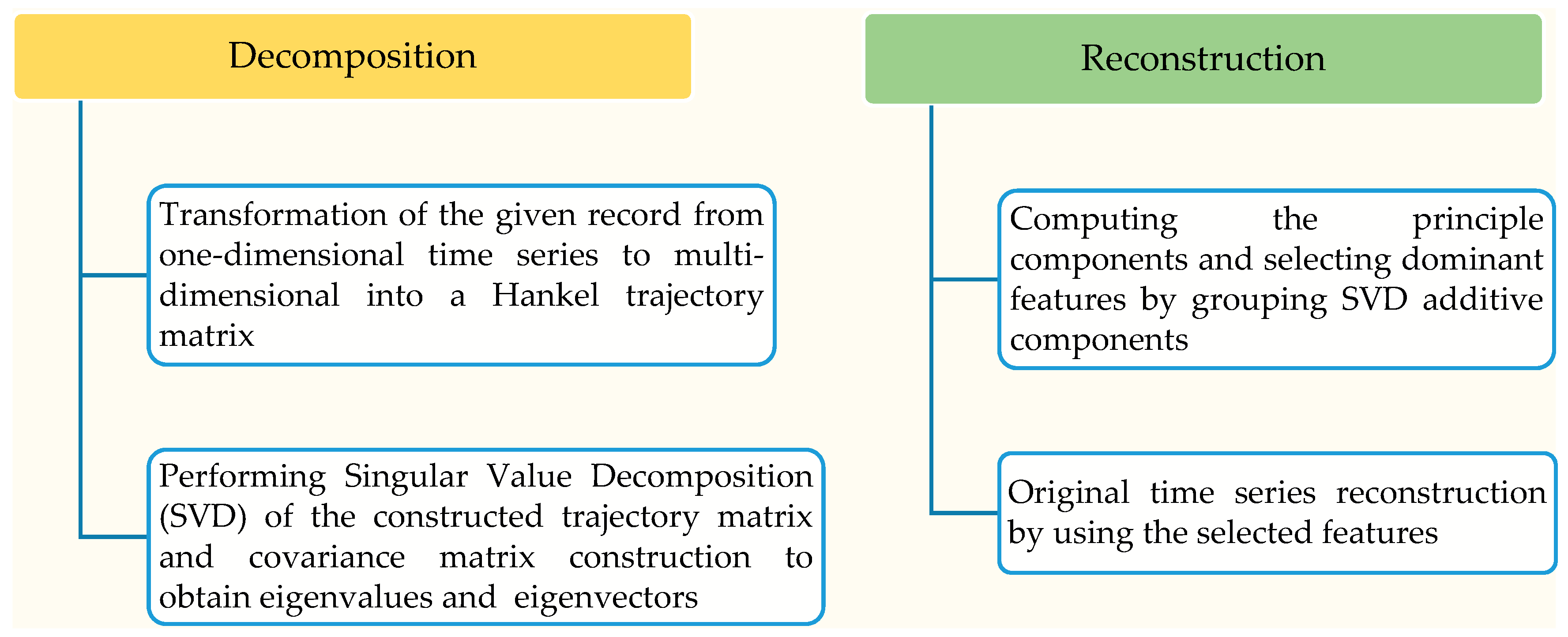
The idea of the SSA is based on the decomposition of a time series into a number of subseries, so that each subseries can be identified into different groups as; oscillatory components, a trend or noise. The SSA is a model free and non-parametric method consists of two complementary stages which are decomposition and reconstruction [27,29,40,41], as shown in Figure 1. The method is mainly based on statistical approaches and many basic operations of the SSA algorithm are elementary linear algebra [12,31,40,42].

The key element in the de-nosing process is to remove the noise without losing a significant portion of the signal and this can be accomplished with the SSA [12,33]. The SSA can provide an important concept from the time series known as statistical dimension. The statistical dimension of the process from which the time series was taken is defined as the number of eigenvalues before the noise floor. This concept develops the use of the SSA as a de-noising technique [33]. The main aspect in studying the properties of the SSA is the separability, which describes how well different components can be separated from each other [23,27,43]. If the dataset is separable, the focus of attention must be how to select proper grouping criteria after identifying suitable window length [12,40].

In the SSA method there are some useful insights to be observed. A harmonic component commonly produces two eigentriples with close singular values; however, a pure noise series typically produces a gradually decreasing sequence of singular values. Furthermore, checking breaks in the eigenvalue spectra is also another useful insight [12,27,40,44]. This can be accomplished by using visual SSA tool in the eigenvalue spectra. In other words, checking breaks is to ensure the availability of eigentriples with nearly equal and close singular values when specifying a threshold of such equality. Large breaks among the eigenvalues pairs in the eigenvalue spectra cannot lead to produce a harmonic component [40,44].

In addition to the perception of the typical shape of the eigenvalue spectra, the analysis using w-correlation matrix is used to distinguish between frames containing mostly the energy of the wanted signal and wind-only frames (in our case) presented in the lower end of the spectra.

3.2. The SSA Theory

The term “singular spectrum” came from the spectral (eigenvalue) decomposition of a given matrix A into a set (spectrum) of eigenvalues and eigenvectors. These eigenvalues denoted by λ are specific numbers that make the matrix $A-\lambda I$ singular when the determinant of this matrix is equal to zero. In this mathematical illustration, matrix I is the identity matrix. Singular spectrum analysis, per se, is, the analysis of time series using the singular spectrum. Therefore, the time series under investigation needs to be embedded in a so-called trajectory matrix [27,33].

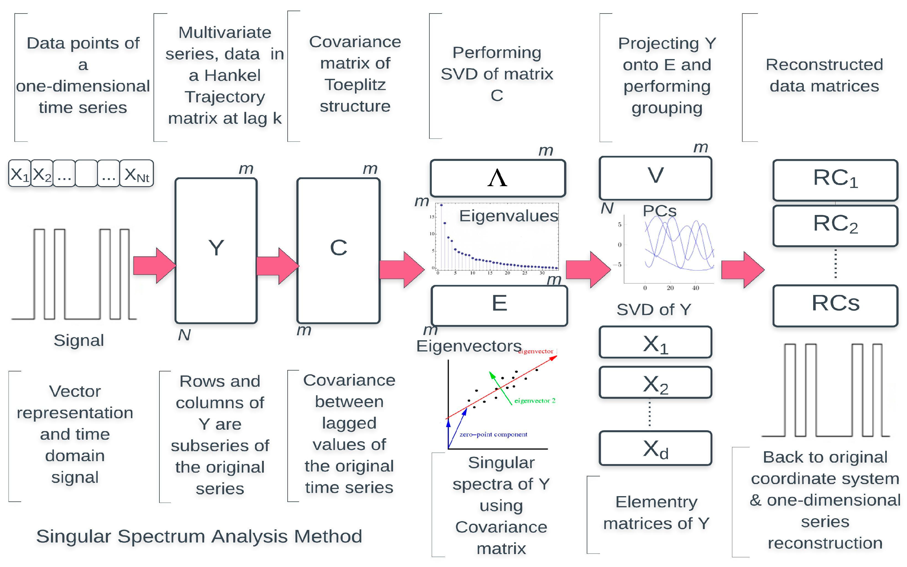
Importantly, the SSA utilises a representation of the data in a statistical domain which called eigen domain rather than a time or frequency domain. In the SSA method, data is projected onto a new set of axes that fulfil some statistical criterion and might change according to the change of the structure of the data over time [27,45]. Figure 2 illustrates a descriptive process of the SSA method.

In principal, the idea of the SSA is to embed a time series $X(t)$ into multi-dimensional Euclidean space and find a subspace corresponding to the sought-for component as a first stage. At the first decomposition stage, the time series is decomposed into mutually orthogonal components after computing the covariance matrix from constructed trajectory matrix. The trajectory matrix is obtained from the real observations of the time series and decomposed into elementary matrices or additive components [21,27,40]. The (SVD) method is used to determine the principal components of a multi-dimensional signal [45]. The aim is to decompose the original time series or the time signal captured by sensors into a small number of independent and interpretable components such as; a slowly varying trend, oscillatory components (harmonics) and a structure less noise [30,46].

Once the SSA decomposes mixed signals in the eigen-subspaces, it selects and groups the principle components according to their contributions to noise and wanted signals in the singular spectrum domain. Eventually, the second stage is to reconstruct a time series component corresponding to this subspace [27,40]. The second stage entails the reconstruction of the signal into an additive set of independent time record [30]. The SSA reconstructs the wanted components back to the time domain resulting in the separation of noise and wanted signals. The reconstruction of the original time series is accomplished by using estimated trend and harmonic components [46]. The time series is reconstructed by selecting those components that reduce the noise in the series [47].

3.3. Mathematical Formulation of the SSA Method

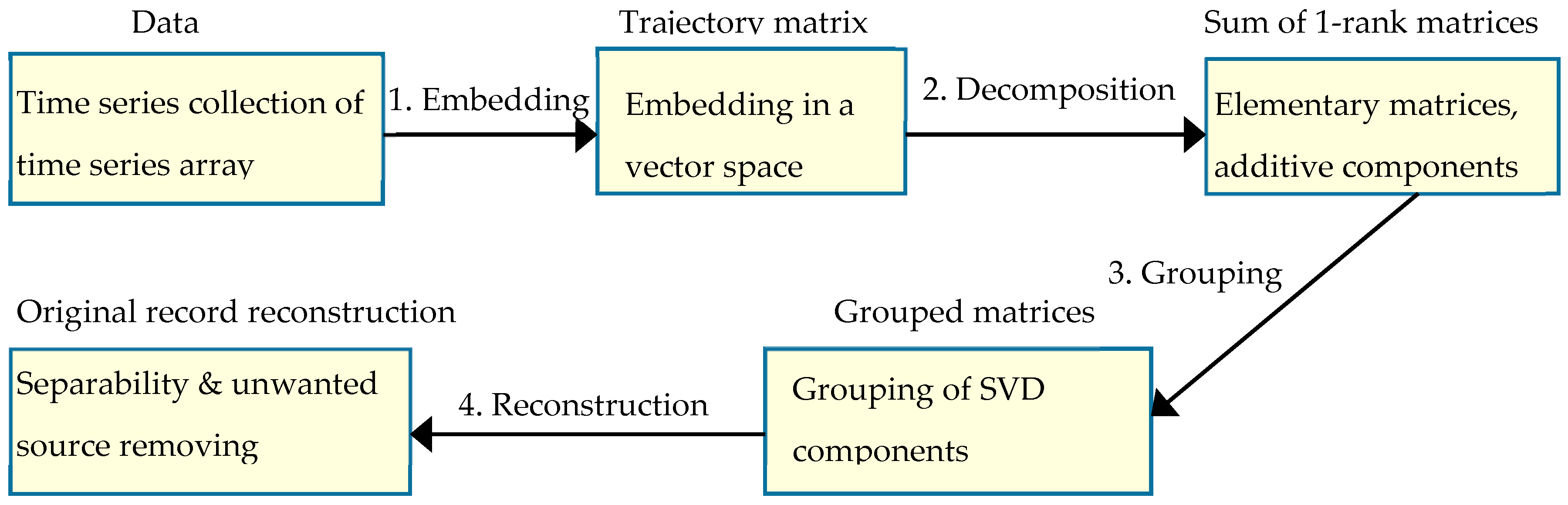
Time series can be stored in a vector denoted by X for example, where the entries are the data points that describe the time series as a sequence of discrete-time data [31]. Such vector is an introductory element to many further steps as it includes the required information about the time series. The SSA method is basically consists of main four steps [24,29,48]. Figure 3 shows these steps which will be explained with many important aspects in the next subsections.

3.3.1. Embedding Process

• Step One: Vector Representation
  In practice, the SSA is nonparametric spectral method based on embedding a given time series {X(t): t = 1, …, N_t} in a vector space. The vector X, whose entries $N_t$ are the data points of a time series, can clearly define and describe this time series at regular intervals [27,30,40]. If we consider a real-valued time series X(t) = (x₁, x₂, …, x_Nt) of length $N_t$ and x₁, x₂, …, x_Nt data points, therefore, the given time series can simply be represented as a column vector as shown in Equation (1):

  $$X^T=(x_1,x_2\dots \dots .x_{N_t}),$$

  (1)
  This column vector shows the original time series at zero lag (i.e., when there is no delay, $k=0$). At a given window length m, the lag k can therefore be expressed in the range from 0 to m − 1 in a 1 lag shifted version as in Equation (2):

  $$k=0,1,\dots \dots ,m-1,$$

  (2)
  Hence, the window length m should be suitably identified in order to obtain the lag k which needed to construct a new matrix according to delay coordinates.
  In SSA jargon, this matrix is called “embedded time series” or trajectory matrix and denoted by Y. The window length is also called embedding dimension and it represents the number of time-series elements in each snapshot [27,30,33,40].
  The whole procedure of the SSA method depends upon the best selection of this parameter as well as the grouping criteria. These two key aspects are very important to develop the concept of reconstructing noise free series from a noisy series. Different rank-one matrices obtained from the SVD can be selected and grouped in order to be processed separately. If the groups are properly partitioned, they will reflect different components of the original time record [27,40].
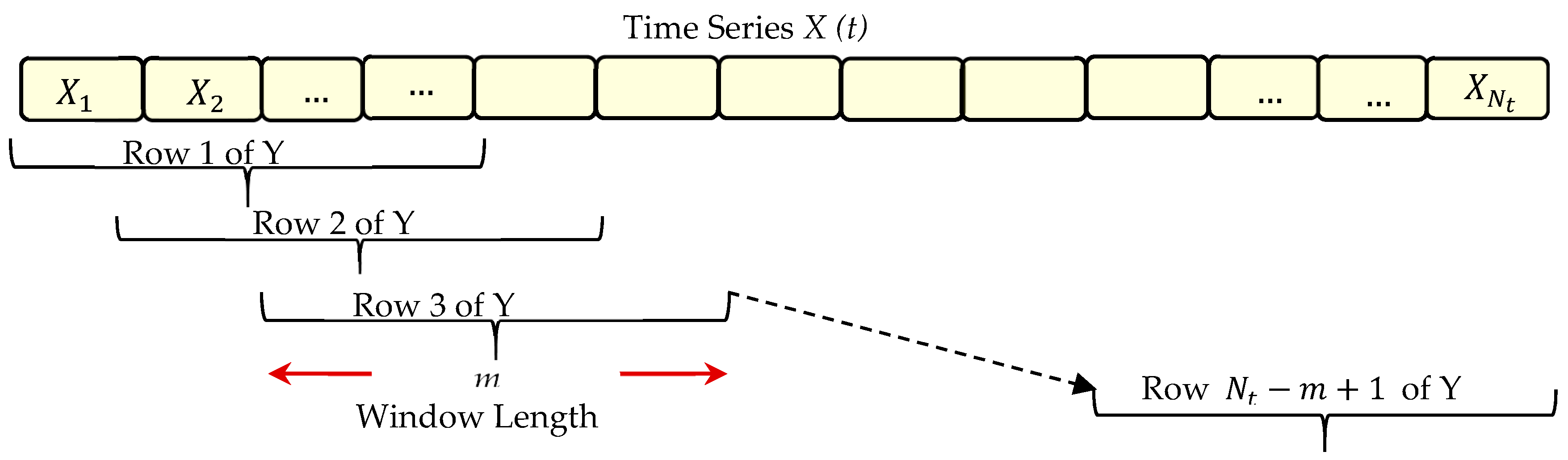
• Step Two: Trajectory Matrix Construction
  The trajectory matrix contains the original time series in the first column and a lag 1 shifted version of that time series for each of the next columns. We can obviously understand from Equation (2) that the column vector shown in Equation (1) is $X(t)$ when $k=0$. As explained in [31], according to delay coordinates, we will obtain a total number of column vectors equals m. Importantly, these vectors are similar in size to the first column vector but with a 1 lag shift at $k=1$, $k=2$, up to $k=m-1$. This assumption is given when the last rows are supplemented by 0s based on the delay as a first method.
  In the second method, arranging the snapshots of any given time series as row vectors can lead to construct the trajectory matrix when the last rows are not supplemented by 0 s [27,40]. To simplify, we assume for example, an embedding dimension $m=4$, therefore according to Equation (2), only lags of $k=0$, 1, 2 and 3 will be considered. However, in this case, a trajectory matrix Y of size N × m will be constructed as in Equation (4). For more clarification, we consider a representation of any given time series $X(t)$ according to our assumption $m=4$ as depicted in Figure 4.
  The coordinates of the phase space can be defined by using lagged copies of a single time series [33]. The trajectory matrix corresponds to a sliding window of size m that moves along the time series $X(t)$ [12,40]. Since the sliding window has an overlap equals $m-1$ as shown in Figure 1 and values of k according to Equation (2), therefore the number of rows of Y which can be filled with the values of $X(t)$ is denoted by N and can be calculated by Equation (3):

  $$N=N_t-\left(m-1\right)=N_t-m+1,$$

  (3)

  where $N_t$ is the number of data points, m is the window length and $m-1$ is the overlap.
  As explained in [33], the snapshots of a given record when considering only number of rows of Y which can be filled with the values of $X(t)$ according to Equation (3) are vectors and can be seen as $V_1^T=\left(x_1,x_2,\dots ,x_m\right)$, $V_2^T=\left(x_2,x_3,\dots ,x_{m+1}\right)$ up to $V_N^T=\left(x_N,x_{N+1},\dots ,x_{N_t}\right)$. Hence, the trajectory matrix can be constructed by arranging the snapshots as row vectors and only N_t − m + 1 rows can be filled with values of $X(t)$ as in Equation (4):

  $$Y=1/\sqrt{N}\left[\begin{array}{c}{V}_1^T\\ V_2^T\\ V_3^T\\ ⋮\\ V_N^T\end{array}\right]=1/\sqrt{N}\left[\begin{array}{ccccc}{x}_1& x_2& x_3& \dots & x_m\\ x_2& x_3& x_4& \dots & x_{m+1}\\ x_3& x_4& x_5& \cdots & x_{m+2}\\ ⋮& ⋮& ⋮& \ddots & ⋮\\ x_N& x_{N+1}& x_{N+2}& \cdots & x_{N_t}\end{array}\right],$$

  (4)

  where $\sqrt{N}$ is the convenient normalisation.
  The constructed trajectory matrix includes the complete record of patterns that have occurred within a window of length m. To generalise, we assume that $X(t)$ is a given time series and t = 1, 2, 3, …, N_t, the augmented or trajectory matrix is constructed as in Equation (5):

  $$Y=\left[\begin{array}{ccc}{X}_1:& \dots & :X_m\end{array}\right]={(x_{ij})}_{i,j=1}^{N,m},$$

  (5)

  where the columns vectors of this matrix $X_i^T=\left(x_i,\dots ,x_{i+N-1}\right)$, the entries $x_{ij}=x_{i+j-1}$, $1\le i\le N$, $N=N_t-m+1$ and $1\le j\le m$.
  The arrangement of entries $x_{ij}$ of the trajectory matrix depends on the lag, considering that the trajectory matrix has dimensions N by m. The trajectory matrix and its transpose $Y^T$ are linear maps between the spaces $R^m$ and $R^N$ [40]. Two important properties of the trajectory matrix are stated in [49], the first is that both the rows and columns of Y are subseries of the original series. The second is that Y has equal elements on anti-diagonals; makes it a Hankel matrix (i.e., all the elements along the diagonal i + j = const are equal).

3.3.2. Covariance Matrix Construction

The covariance matrix is basically a matrix that shows the covariance between the values $X(t)$ and $X(t+k)$ which mainly the covariance between lagged (or “delayed”) values of the original time series $X(t)$ [27,40]. According to [50], there are two methods of computing the covariance matrix. Estimating the lag-covariance matrix directly from the data is one method. The covariance matrix is a square matrix of dimension m × m and considered as a Toeplitz matrix with constant diagonals. The entries c_ij of this matrix depend only on the lag $\left|i-j\right|$ as in Equation (6) [46].

$$c_{ij}=\frac{1}{ N_t-\left|\mathrm{i}-\mathrm{j}\right|}{\sum }_{t=1}^{ N_t-\left|\mathrm{i}-\mathrm{j}\right|}X\left(t\right)X\left(t+\left|\mathrm{i}-\mathrm{j}\right|\right),$$

(6)

where $N_t$ represents the number of data points, the entries c_ij when $\left|i-j\right|=0$ for $i=j$, are the entries across the main diagonal (i.e., their values are typically closed to 1).

As a second method, the lagged-covariance matrix can be computed form the trajectory matrix Y and its transpose [33]. The variances of each column of Y are presented in the main diagonal of the covariance matrix. As a general mathematical representation, the covariance matrix can be also written, as in Equation (7):

$$\mathrm{C}=\frac{1}{N}\sum _{i=1}^N{Y}_i{Y}_i^T,$$

(7)

C is the covariance matrix of the snapshots from the original time record of order $m\times m$, its elements are all real numbers and $c_{ij}=c_{ji}$ for all $i$ and $j$, thus it is symmetric $C=C^T$.

3.3.3. Computing the Eigenvalues and Eigenvectors

To obtain spectral information on the time series, the SSA proceeds by diagonalising the covariance matrix. Spectra decomposition is a factorisation of a diagonalisable matrix into a canonical form, whereby the representation of the matrix is in terms of its eigenvalues and eigenvectors [33,40].

• Finding the Eigenmodes
  Finding the eigenvalues and eigenvectors or the so-called eigenmodes is based on the fundamental question of eigenvector decomposition. In general, this question is for what values is the matrix $A-\lambda I$ singular? Such question of singularity regarding matrices can be answered with determinants [33,40]. Using determinants, however, the fundamental question which just has been asked above can be reduced to; for what values of $\lambda$ is the determinant of the matrix $A-\lambda I$ equals to zero? or as in Equation (8):

  $$\det \left(A-\lambda I\right)=0,$$

  (8)
  This is called the characteristic equation for the matrix A where ${\lambda }^{\prime }s$ that make the matrix $A-\lambda I$ singular are called eigenvalues [33]. The eigenvalues of this matrix can therefore be found by solving the characteristic equation.
  For each of these special values there is a corresponding set of vectors called the eigenvectors of A and should satisfy Equation (9):

  $$\left(A-\lambda I\right)X=0,$$

  (9)
  Equation (9) can be written as $AX=\lambda X$. Vector $X$ represents a set of eigenvectors $X_n$ correspond to ${\lambda }^{\prime }s$.
  When representing the eigenvectors geometrically, they can be considered as the axes of a new coordinate system. Hence, any scalar multiple of these eigenvectors is also an eigenvector of matrix A [27]. To simplify, all eigenvectors of the form $C{X}_n$ ($C$ is scalar) will form an eigen-subspace spanned by $X_n$, which means that the eigen-subspace is one-dimensional and is spanned by $X_n$. In this case, only the scale of the eigenvectors is changing while their direction remains unchanged. The process of decomposition can be simplified as matrix A is usually symmetric with real coefficients. The eigenvalues and eigenvectors can be seen as a way to express the variability of a set of data [50].
• Diagonal Form of the Covariance Matrix
  The covariance matrix C is an n by n symmetric matrix with n linearly independent eigenvectors $(e_i)$, $i=1,\dots ,n$; hence a matrix E, whose columns are the eigenvectors of C, can be constructed and satisfies Equation (10):

  $$E^{-1}CE=\mathsf{\Lambda },$$

  (10)
  The product on the left-hand side of Equation (10) is called the diagonal form of C and therefore Λ is a diagonal matrix whose nonnegative entries are the eigenvalues of C.
  The eigenvectors of C should be linearly independent in order to make C diagonalisable in this way. Also matrix E is not unique because the eigenvectors can always be multiplied by a constant scalar preserving their nature as eigenvectors [33].
• Spectral Decomposition
  We assume C is a real symmetric matrix where $C=C^T$. Now, in this case, every eigenvalue of C is also real and if all eigenvalues are distinct, then their corresponding eigenvectors are orthogonal. Our real, symmetric matrix C can therefore be diagonalised by an orthogonal matrix E whose columns are the orthonormal eigenvectors of C [44]. It is important now to state a principal theorem when there is a diagonalizable matrix E whose columns are orthonormal of a real and symmetric matrix C.
  Since $E^{T}E=I$ and $E^T=E^{-1}$, then Equation (10) can be rewritten as:

  $$C=E\mathsf{\Lambda }{E}^T,$$

  (11)
  Matrices Λ and E can be seen as:

  $$\mathsf{\Lambda }=\left[\begin{array}{cccc}{\lambda }_1& 0& \dots & 0\\ 0& {\lambda }_2& \cdots & 0\\ ⋮& ⋮& \ddots & ⋮\\ 0& 0& \cdots & {\lambda }_m\end{array}\right], E=\left[\begin{array}{cccc}{e}_1^1& e_1^2& \dots & e_1^m\\ e_2^1& e_2^2& \cdots & e_2^m\\ ⋮& ⋮& \ddots & ⋮\\ e_m^1& e_m^2& \cdots & e_m^m\end{array}\right],$$

  (12)
  Matrix Λ is symmetric with entries ${\lambda }_i$ along the leading diagonal for $i=1,\dots \dots ,m$, however $E^k$ is the corresponding normalised column eigenvector for $k=1,\dots \dots ,m$ as well. The eigenvectors matrix consists of a set of column vectors with entries $e_j^k$ that represent the j^th component of the k^th eigenvector. Once we conserve our matrices square, then we have $j=k=1,\dots \dots ,m$. The diagonal matrix Λ consists of ordered values $0\le {\lambda }_1\le {\lambda }_2\le \dots \le {\lambda }_m$ [21,22,27].
• The Singular Spectrum
  The square roots of the eigenvalues of matrix C are called the singular values of the trajectory matrix [27,28,33]. These ordered singular values are referred to collectively as the singular spectrum. From the (SVD), the trajectory matrix can be written as:

  $$Y=US{E}^T$$

  (13)

  where U and E are left and right singular vectors of Y and S is a diagonal matrix of singular values.
  The singular spectrum of Y consists of the square roots of the eigenvalues of C which called the singular values of Y with the singular vectors being identical to the eigenvectors that given in matrix E [33]. The decomposition of matrix C can also be performed by substituting Equation (13) in the form $C=Y^{T}Y$ to yield $C={(US{E}^T)}^T(US{E}^T)$$=ES{U}^{T}US{E}^T$. Since $U^{T}U=I$, we find:

  $$C=E{S}^2{E}^T$$

  (14)
  For the decomposition being unique, it follows that $S^2=\mathsf{\Lambda }$. The right singular vectors of Y are the eigenvectors of C and the left singular vectors of Y are the eigenvectors of the matrix $Y{Y}^T$ [27,40]. Importantly, the number of eigenvalues is equal to the window length and in turn the number of the associated eigenvectors that matrix E contains [33].

3.3.4. Principle Components

The eigenvectors of C can be used to compute the principal components (PCs) with entries $a^{k\prime }s$ by projecting the original time series onto matrix E. This process can be given by Equation (15):

$$a_i^k=\sum _{j=1}^m{x}_{i+j-1}{e}_j^k$$

(15)

where $a_i^k$ represents the principle components arranged in columns $k$ and rows $i$ for $[i=1,2,\dots ,N]$ as each element of the matrix V results from multiplying a row of Y by a column of E, $x_{i+j-1}$ represents the incremental elements in the rows of Y, $e_j^k$ represents the j^th component of the k^th eigenvector in the matrix E [21,22].

For each value of $i$, the summation will stop when $j=m$ and this repetitive procedure ends when $i=N$. The resultant matrix V will be of dimension $N\times m$ as in Equation (16):

$$V=YE=\left[\begin{array}{cccc}{a}_1^1& a_1^2& \dots & a_1^m\\ a_2^1& a_2^2& \cdots & a_2^m\\ ⋮& ⋮& \ddots & ⋮\\ a_N^1& a_N^2& \cdots & a_N^m\end{array}\right],$$

(16)

The columns of V do not correspond to different time lags as in the trajectory matrix. Rather, in the SSA method, the principle components matrix is introduced as a projection of the embedded time series onto the eigenvectors. The original values of Y have been projected in a new coordinate system for gathering the variance in the principle components [27,51].

3.3.5. Reconstruction of the Time Series

We can return from the eigen domain to time domain by projecting the PCs onto the eigenvectors. Applying such projection can help us in obtaining time series in the original coordinates referred to as the Reconstructed Components (RCs). The RCs that resemble the original time series are the ones correspond to the PCs with substantial contribution to the wanted signals in the singular spectrum domain. It is significant, however, to choose a group $I$ of indices of the eigenvectors based on the standard SSA recommendations to avoid missing part of the signal or adding part of the noise [27,51].

To do that, we need to reconstruct a new matrix denoted by Z in a similar way of constructing the trajectory matrix but the dominant principal components will be used and time delay runs in the opposite direction. According to [46], the part of a time series that is associated with a single or several m eigenvectors of the lag-covariance matrix can be reconstructed by combining the associated principle components, as in Equation (17):

$$R{C}_{\mathcal{K}}\left(t\right)=\frac{1}{m}\sum _{k\in \mathcal{K}} \sum _{j=L_t}^{U_{\mathcal{K}}}a\left(t-j+1\right)e_k\left(j\right),$$

(17)

where $\mathcal{K}$ is a set of eigenvectors on which the reconstruction is based, m is the normalisation factor which is the window length, $U_{\mathcal{K}}$ and $L_t$ are the upper and lower bound of summation which may differ from the central part of the time series and its end point as stated in [52], $a(t-j+1)$ are rows entries of Z, $e_k(j)$ are columns entries of E.

Each RC retranslates its corresponding principal component from the eigen-subspace into the original units of the time series. Importantly, from such reconstructions, the time series can be reduced to oscillatory components that correspond to the most dominant eigenvalues with high variance and noise components that correspond to the end region of eigenvalues spectra [27,40].

4. The SSA Algorithm

4.1. Description of the SSA Algorithm

The SSA algorithm involves the decomposition of a time series and reconstruction of a desired additive component. The SSA algorithm can be outlined in several steps as follows.

4.1.1. Signal Decomposition

The algorithm generates a trajectory matrix from the original time series $X(t)$ by sliding a window of length m. With the SSA, every time series can be decomposed into a series of elementary matrices after mapping it into trajectory matrix. Each of these matrices shows glimpses of a particular signature of oscillation patterns. The trajectory matrix is then approximated using SVD. A one-dimensional time series shown in Equation (18) can be transferred into a multi-dimensional series in the embedding step which can be viewed as a mapping process.

$$X\left(t\right)=x_1,x_2,\dots \dots ,x_{N_t}$$

(18)

The multi-dimensional series contains vectors $X_k$ which called m-lagged vectors (or, simply, lagged vectors) as in Equation (19):

$$X_k^T=\left(x_{k+1},x_{k+2},\dots \dots ,x_{k+\left(N_t-m+1\right)}\right)$$

(19)

We then consider Y as multivariate data with m characteristics and N observations. In this embedding step, the single parameter is the window length which is an integer such that $2\le m\le N_t$. The result of the embedding process is a Hankel trajectory matrix Y with entries ${(x_{ij})}_{i,j=1}^{N,m}$. The columns $X_j$ of Y are vectors lie in m-dimensional space $R^m$ [39]. Then the embedded time series can be seen as:

$$Y=\left[\begin{array}{ccc}{X}_{k=0},& \dots \dots & ,X_{k=m-1}\end{array}\right]$$

(20)

4.1.2. Computing the Diagonal Matrix C

This step is the preparation for applying the SVD. Matrix C can be computed using the trajectory matrix and its transpose or using a specified MATLAB function that gives a vector of size m.

4.1.3. Performing SVD of Matrix C

It is a step of computing the diagonal values and their corresponding vectors where each represented in a separate matrix.

4.1.4. Computing the Principle Components and Performing Grouping

A matrix that contains the PCs is introduced as the projection of the embedded time series onto the eigenvectors in the eigen-subspace. The selected groups of the PCs are presented in vectors and can be aligned in a single matrix. Grouping corresponds to splitting the elementary matrices $X_i$ into several groups and summing the matrices within each group. The SVD of Y can be written as a set of elementary matrices and performed as in Equation (21):

$$Y=X_1+X_2+\dots +X_d,$$

(21)

where $X_i=\sqrt{{\lambda }_i}{E}_i{V}_i^T$ are the additive components or elementary matrices of Y for $i=1,\dots ,d$ and $d$ is the number of non-zero eigenvalues of $Y{Y}^T$.

The number of elementary matrices is denoted by r. $E_1,\dots ,E_d$ are the orthonormal system of the associated eigenvectors and $V_1,\dots ,V_d$ are the principle components, $(\sqrt{{\lambda }_i},E_i,V_i)$ is the $i^{th}$ eigentriple of Y.

4.1.5. Reconstruction the One-Dimensional Series

The RCs can be computed by projecting the principle components presented in matrix Z onto the eigenvectors of matrix E when the normalization is considered and hence the process as in Equation (22):

$$RCs=\frac{1}{m}ZE,$$

(22)

The RCs can also be calculated by inverting the projection of the principle components onto the eigenvectors transpose matrix as in Equation (23):

$$RCs=YE{E}^T,$$

(23)

A group of r eigenvectors with $1\le r\le d$ defines an r-dimensional hyperplane in the m-dimensional space $R^m$ of vectors $X_i$. The projection of Y into this hyperplane will approximate the original matrix Y.

4.2. Parameters of the SSA Algorithm

The SSA technique depends upon two important parameters which are the window length m, which is the single parameter in the decomposition stage and the number of elementary matrices r. According to [12], the window length is highly related to spectral information or the frequency width that corresponds to each principle component.

There is no general rule for the choice of the window length since the selection depends on the initial information on the time record and the problem of interest [38]. As stated in [53], the choice of the window length parameter used for decomposition and the grouping of SVD components used for reconstruction can totally effect the output time series. It is important, however, to select values of m and the $I$ groups of the eigenvectors to ensure better separability [42]. The performance of the SSA algorithm is highly dependent on the selection of the window length [21,54].

In spite of the greater computation burden due to bigger sized matrix, it has been recommended that m should be large enough but not greater than $N_t/2$ in order to significantly represent separated components and obtain satisfied results [12,55]. Whereas, other studies reported that it should be larger than $N_t/2$. We can always assume $m\le N_t/2$ as this value has been regarded as the most interesting case in practice. In spite of the considerable attempts and various methods that have been considered for choosing the optimal value of m, there is inadequate theoretical justification for such selection [12,40,47]. Whereas, according to [33], m can be computed as $N_t/4$ and considered as a common practice. Smaller values can be considered if the purpose is to extract the trend even when the time series is short (small $N_t$). A method of selecting window length is descried in [12] and a detailed description of selecting these parameters is given in [49].

Importantly, we should try to achieve appropriate separability of the components as an important rule in selecting m. Hence, the decomposition stage of the SSA delivers significant results if the resulting additive components of the time series are approximately separable from each other [21,43]. The improper selection of m and r would imply an inferior decomposition and in turn inaccurate results will be produced [21,22].

We will miss a part of the signal if r is smaller than the true number of eigenvalues (under fitting) and therefore the reconstructed series becomes less accurate. Otherwise, if r is too large (overfitting), then a part of noise together with the signal will be approximated in the reconstructed series [56].

4.3. Grouping and Separability

The representation of an observed series as a sum of interpretable components, which mainly are trends, periodicals or harmonics with different frequencies and noise along with the separation of such components, is always considered as an issue of concern in time series analysis. With the SSA, this problem can be solved, trends can be extracted and harmonic signals can be separated out from noise. The idea is based on applying suitable grouping approach to the SVD components matrix in order to transform back to time series expansion from the expansion of grouped matrix. The separability of the components of the time series can therefore be defined as the ability of allocating these components from an observed sum when appropriate grouping criteria is applied [27,43,57]. The SSA decomposition relies on the approximate separability of the different components of the time record [21,38].

For splitting the indices $1\le r\le d$ of the r group of eigenvectors into I groups that’s adequate to achieve the separability, r has to be clearly specified. In this paper, we consider only two groups; one associated with the signal and the other associated with wind noise. In this case, group $I=\left\{1,\dots ,r\right\}$ with the related elementary matrices, which will be $X_I=X_1+X_2+\dots +X_r$, are associated with the first group that represents the signal. The second group $\overline{I}=\left\{r+1,\dots ,d\right\}$ and the related elementary matrices $X_{\overline{I}}=X_{r+1}+X_{r+2}+\dots +X_d$, represent the noise. In other words, the rest of vectors $(d-r)$ is not of interest as they represent noise [40,43,44,54].

A quantity known as weighted correlation or simply (w-correlation) and defined as a natural measure of the dependence between the reconstructed components can be used to achieve the separability. Well separated reconstructed components are the ones that have zero w-correlation. Whereas, reconstructed components with large values of w-correlation should be considered as one group as this corresponds to the same component in the SSA decomposition [21,29,54].

The plot of the singular spectra, which shows the eigenvalues ${\lambda }_1,\dots ,{\lambda }_d$, can give an overall observation of the eigenvalues to decide where to truncate the summation of the additive components in Equation (21) for building a good approximation of the original matrix. Importantly, similar values of the $\lambda \prime s$ can give an identification of the eigentriples which correspond to the same harmonic component of the time series. Furthermore, using periodogram analysis of the original time series can also lead to select the groups. The lower end of the singular spectra typically shows a slowly decreasing sequence of eigenvalues and mainly related to the noise component [44].

It is worthwhile to mention that for smaller eigenvalues, the energy represented along the corresponding eigenvectors is low. Consequently, smallest eigenvalues are commonly considered to be noise. We can, however, remove the unwanted source from the original signal as long as we transform the data back into the original observation space using matrix manipulation in the SSA-based technique. If a truncated SVD of the trajectory matrix Y is performed (i.e., when only the significant eigenvectors are retained), then the columns of the resultant matrix $\tilde{Y}$ are the noise-reduced signal [27,40].

5. Experimental Procedure

5.1. Description of Experiments

A range of experiments were carried out to identify the potential and capability of the SSA in microphone wind noise reduction. Our experimental investigation plan was divided into several phases based on applying an incremental methodology. In the first phase, we performed several experiments for separation of wind noise from many deterministic signals along with the separation of such signals from each other. The SSA algorithm was implemented in the second phase to mitigate wind noise in corrupted speech signals [22].

In the third phase, we moved to sweep tones and environmental sounds, particularly birds’ call. Although in call cases, notable wind noise reduction was observed, results are different from case to case due to the complexity of the environmental sounds. Only results from separation of outdoor wind noise from birds’ chirps are detailed in the current paper. The experimental procedure of the SSA method is shown in Figure 5. The experiments were carried out on MATLAB platform.

There are five main steps in the experimental procedure shown in Figure 5. The first is to prepare our dataset and make it suitable for the experiments as many factors should be taken into account such as the length of the soundtracks, the sampling rate, etc. The second is the mixing stage which is shown as one step but it is mainly an audio mixer model that mixes pre-recorded samples according to their signal intensity. The third is to apply grouping criterion followed by analysing the algorithm’s outputs and eventually evaluating the method by applying objective measures as fourth and fifth steps.

5.2. Dataset

A benchmark database consists of our signals of interest which are birds’ chirps was needed for this study. A freefield 1010, which is a dataset of standardised 10 s excerpts from Freesound field recording, has been selected.

Some effort has been made in order to make the samples suitable to the case through using automatic methods where possible to ensure that all the samples included in the training dataset are pure birds’ chirps. In addition, all silent gaps have been removed from the samples. Our dataset also includes the samples of wind noise as the samples from this dataset have been mixed to generate mixed soundtracks.

In our experiments, we selected a sample from our dataset of audio recordings of birds’ chirps using an average 100 ms frame size of thousands of frames. The processing time of the SSA depends on the length of the given time series and the selected window length. To reduce the processing time of the SSA, the frame by frame processing method has been applied to process the soundtrack samples instead of processing the whole audio file directly.

5.3. Window Length Optimisation

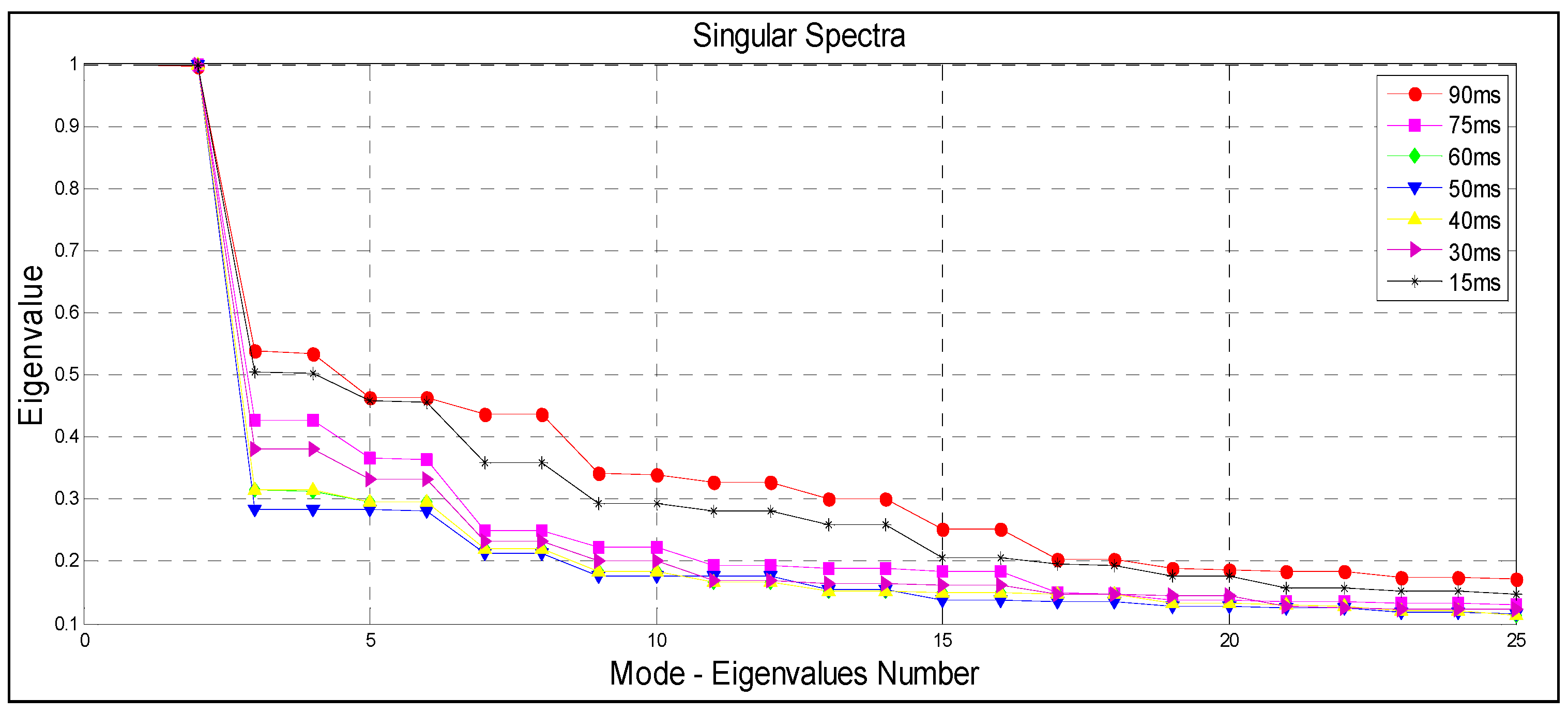
In order to optimise the window length, we calculate singular spectra for our record using seven different window lengths. The selected range of m is between 15 ms and 90 ms based on the size of our frames for the reasons explained above. The size of our frames is 100 ms; however, this range indicates a percentage from 15% to 90% of the new calculated $N_t$.

The processing has to be performed for soundtrack samples of this size considering applying the average method. To perform the calculation of $N_t$ and the multiple suggested window lengths to be entered to the algorithm for the optimisation purpose, we used Equation (24):

$$m_i=p_i{N}_t=p_{i}L{F}_s,$$

(24)

where $m_i$ is the window length, $p_i$ is the desired percentage of the length for $i=1,\dots ,n$, $N_t$ is the new calculated length, $L$ is the frame size in seconds, $F_s$ is the sampling rate in Hertz.

Our audio files are originally 10 s length with a sampling rate of 44,100 samples per second. Figure 6 shows different dominant pairs of nearly equal eigenvalues for almost m = $\frac{1}{4}{N}_t$ to m = $\frac{3}{4}{N}_t$.

A clear break between these singular values and the others, which spread out in a nearly flat noise floor, can also be realised. For the window length above and below this band, indifferent eigenvalues are obtained. Reasonable results can be obtained from the indicated range as still the length $N_t/2$ produces two dominant pairs of nearly equal eigenvalues as illustrated in Figure 6. Thus, the statistical dimension ($d_s$) = 4 seems to be the most dominant value in this case since the record is the superposition of oscillations perturbed by wind noise. Though, these eigenvalues are not always dominant pairs of nearly equal. Dominant eigenvalues in the singular spectrum correspond to an important oscillation of the system for each pair of nearly equal as remarked in [12,33].

6. Results

We selected $m=N_t/2$ as an optimal value for our record, however, since $N_t=4410$ for the 100 ms frames, the window length is therefore equals to 2205. This value also respects the selection rule in the case of harmonic or oscillatory components [38]. Consequently, after performing the SVD of the trajectory matrix, the most dominant eigentriples ordered by their contribution in the decomposition can be obtained.

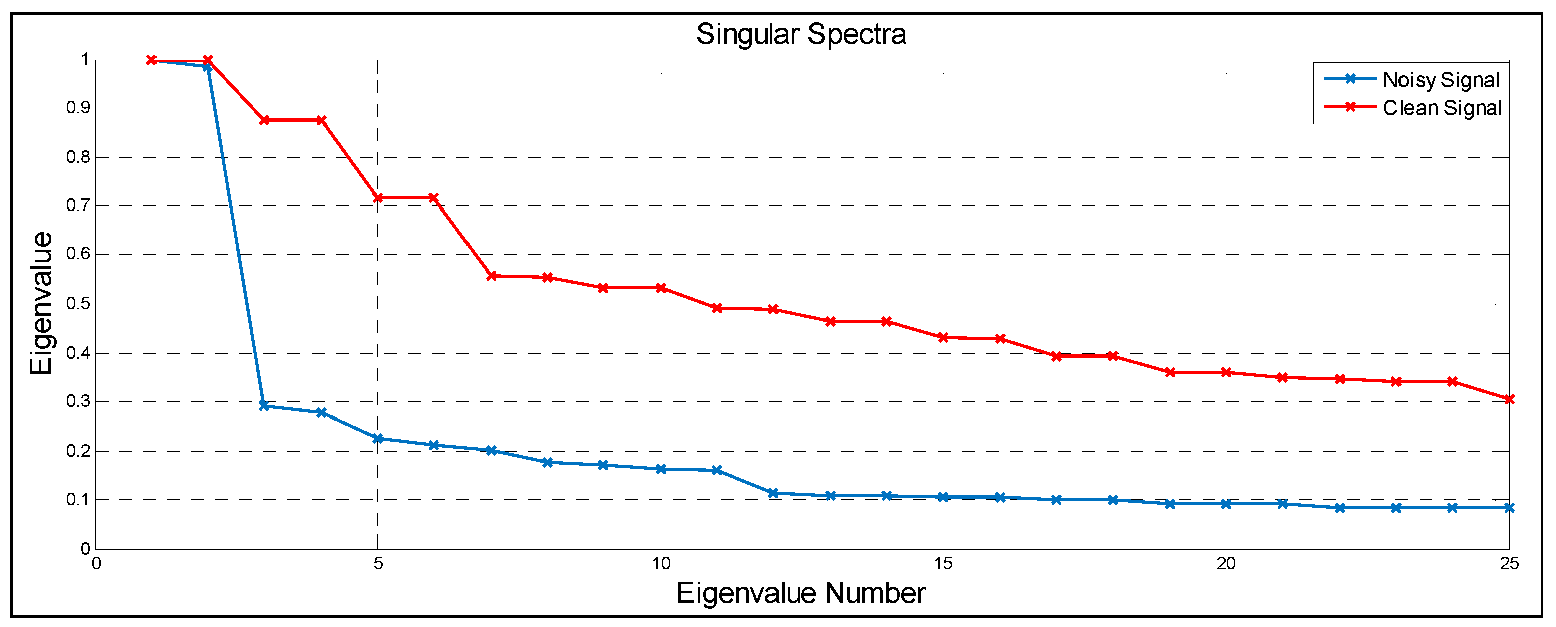
From the plot of logarithms of the singular values shown in Figure 6, a significant drop in values can be seen around component 6 which indicates to the start of the noise floor. Therefore, three obvious pairs are considered as with almost leading singular values. Figure 7 shows the eigenvalues (arranged in descending order) of a decomposed signal of birds’ chirps corrupted with wind noise and a clean one.

Basically, we mixed wind noise with the clean birds’ chirps to obtain the noisy single. We consider the normalisation at scale 1 in the singular spectra to make a valid and fair comparison between the two signals. In the corrupted signal, only first few of the eigenvalues carry large amount of energy. The first pairs of eigenvalues, however, are the ones with less correlation. The high correlation ones are those which left behind and generally represent noise. As illustrated in Figure 7, the equality between the eigenvalues along with equal location of the eigenvalues within the pairs themselves over a specified threshold can be clearly seen in the clean signal. Our grouping technique is based on defining such aspects for the best selection of the most dominant pairs of eigenvalues.

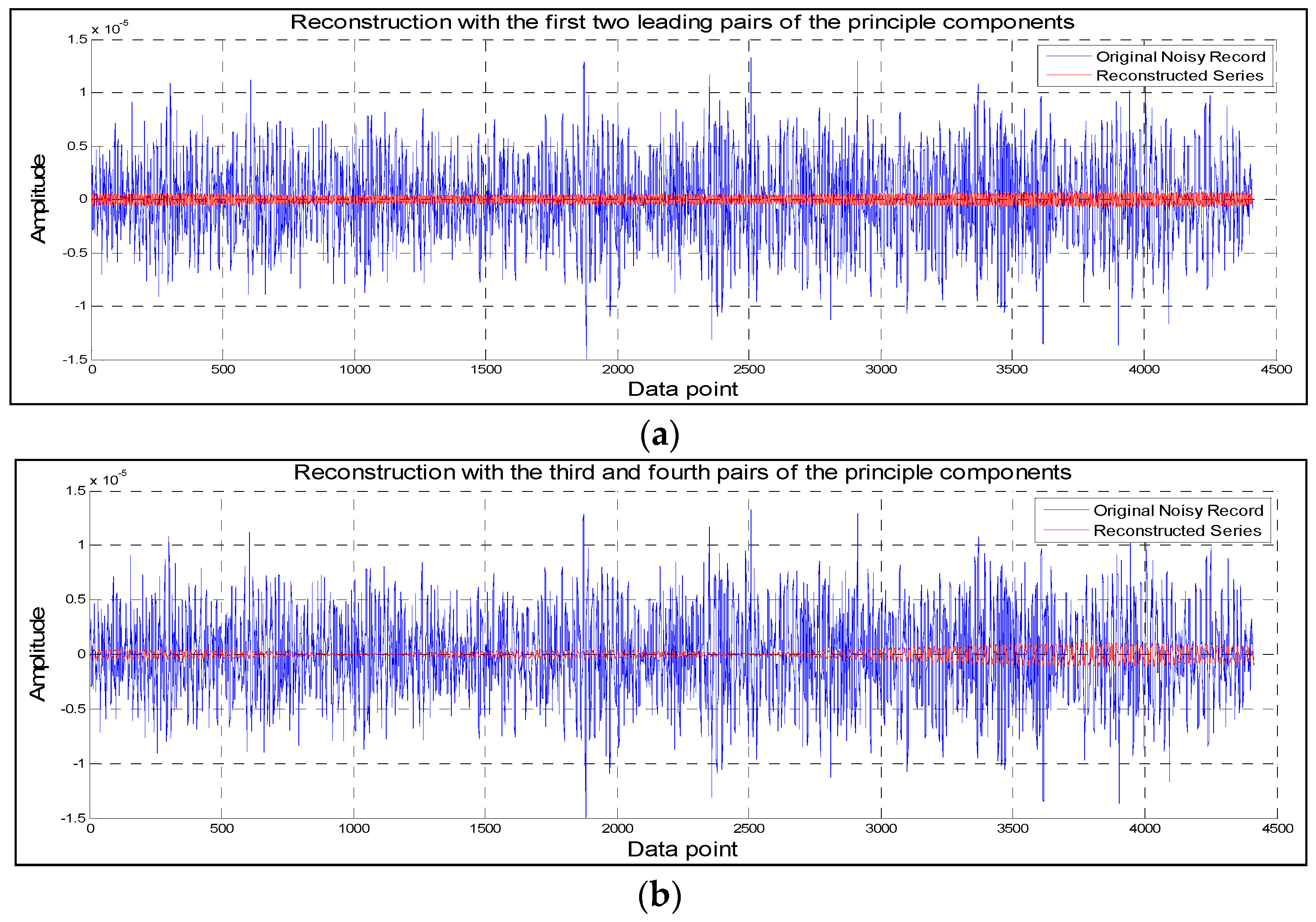
As we wish to retain our signal of interest and separate the wind noise out, the fewest number of eigenvalues before the noise floor will be required. This is based on the contribution of the principle components to the wanted signal and wind noise according to admissible orthonormal bases of eigenvectors. Basically, from the calculation of the singular spectra for our record (with $m=N_t/2$) as shown in Figure 8 we see that, indeed, the first two pairs of eigenvectors correspond to important oscillations and our signal can be reconstructed based on the selection of these pairs in the grouping step.

The phases are in quadrature and regular changes in amplitude are obviously present. In contrast, for the third and fourth pairs, there is slight coherent phase relationship between their two eigenvectors. We always consider the pairs of nearly equal eigenvalues while the others, which spread out in a nearly flat noise floor, are not of interest. However, the eigenvalues associated with these pairs are mostly located in the noise floor of the singular spectra as they are of low variance.

Figure 8 also shows the original noisy signal of our record. The principal components can be computed using the eigenvectors, which is done by projecting the original time series onto the individual eigenvectors. The principal component pairs correspond to the most dominated eigenvectors consist of clean structures of the signal are in marked contrast to the next pairs of principal components, which are noisy with low amplitudes. The grouping therefore has been performed in this way as it has been experimentally found that selecting lower eigenvalues beyond the “elbow” point shown in the singular spectra, which is the start of the noise floor, will only produce noisy signals. Eventually, projecting the principle components onto the orthogonal matrix of the eigenvectors produces the reconstructed components of our record.

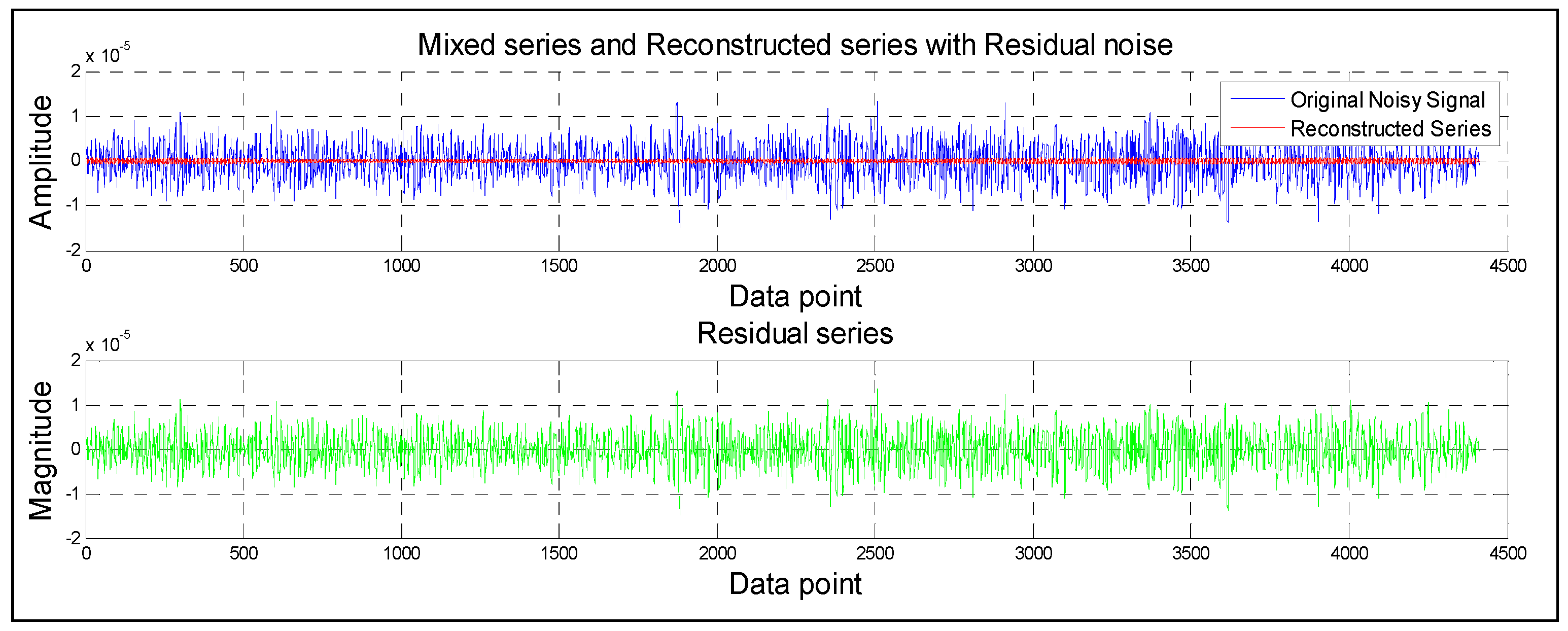
Figure 9 illustrates a comparison of the noisy record, which is a mixture of our signal of interest (bird chirps and wind noise), with the reconstructed one. The differences between reconstructed series and original noisy signal are highlighted in the top part of the figure. It is clear from the bottom part of the figure, a considerable amount of noise (denoted as residual series) was separated out. However, the findings revealed that the de-noised signal resembles the clean one. As seen above, the SSA can readily extract and reconstruct periodic components from noisy time series.

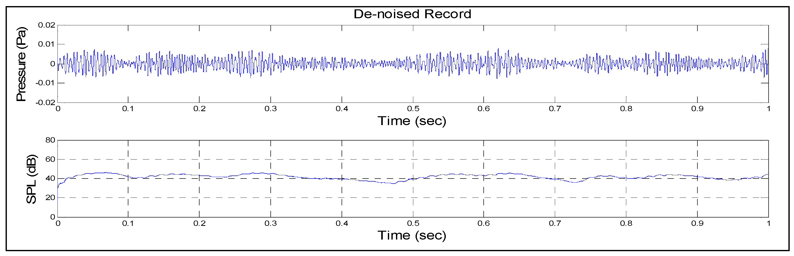
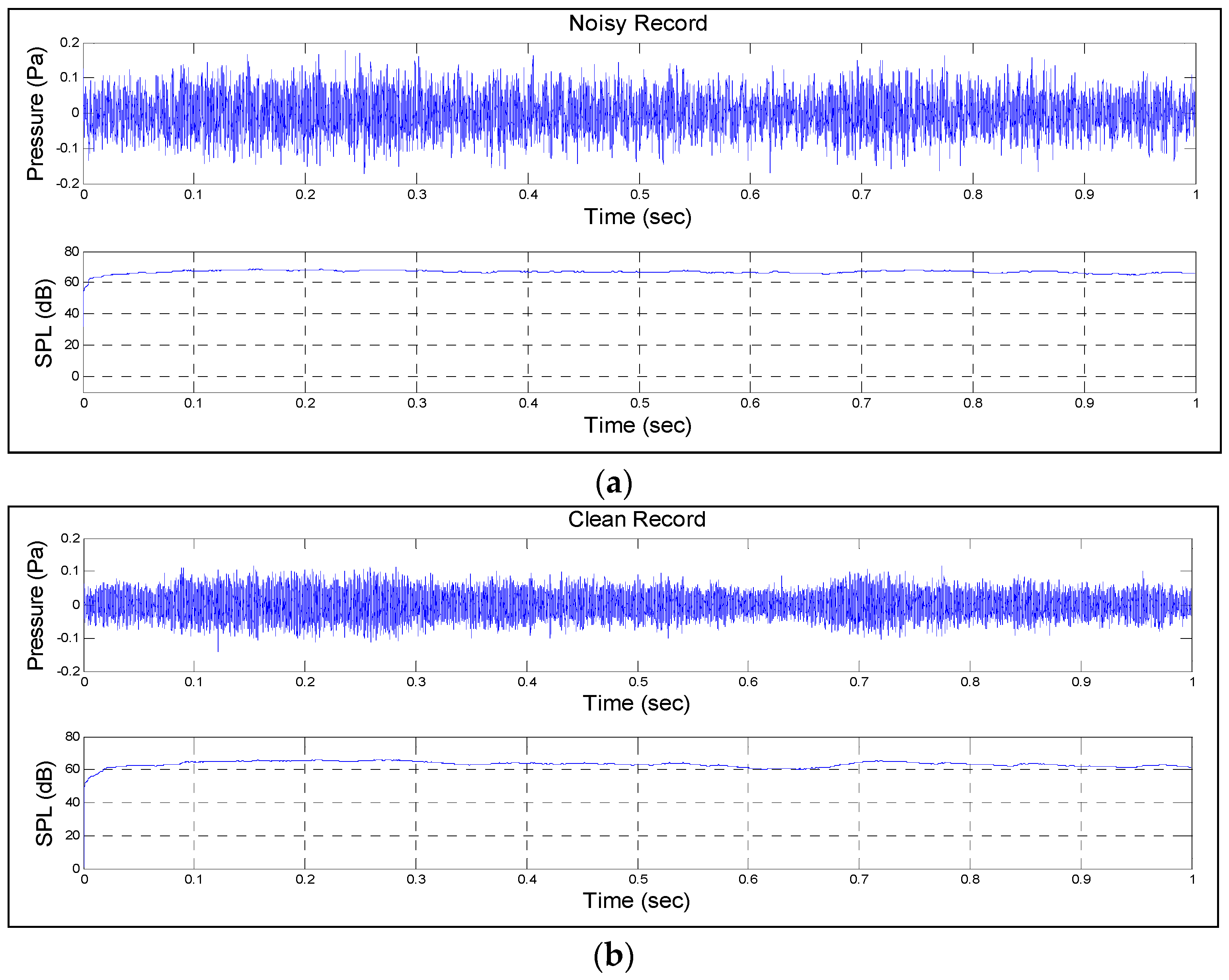
A combination of our signals which are the original birds’ chirps, the mixed signal (bird chirps and wind noise) and the reconstructed signal presented in the time domain with the sound pressure level (SPL) measurement are shown in Figure 10 and Figure 11. The single most striking observation to emerge from the data comparison was that the SSA can reconstruct birds’ chirps.

In the SSA, there are some useful approaches that can be used in the separation of the wanted signal from the noise. In general, a harmonic component produces two eigentriples with close singular values. Using visual SSA tool by checking breaks in the eigenvalue spectra is considered as useful insight. It is worth noting, however, a slowly decreasing sequence of singular values is typically produced by a pure noise time series [43].

Examining the matrix of the absolute values of the w-correlations is another way of grouping. W-correlation matrix contains information that can be very helpful for detecting the separability and identifying grouping. It is a standard way used to check the separability between elementary components. W-correlations can also be used for checking the grouped decomposition. The w-correlation matrix consists of weighted cosines of angles between the reconstructed components of the time series. The number of entries of the time series, which terms into its trajectory matrix, is reflected by the weights [54,57,58].

Basically, the separability between two components such as $X^{\left(1\right)}, X^{\left(2\right)}$ of the time record characterises how well these two components can be separated from each other. Using the w-correlation can help in evaluating the separability and can be simply shown as in Equation (25) [21,38]:

$${\rho }_{12}^{\left(w\right)}=\frac{<X^{\left(1\right)}, X^{\left(2\right)}{>}_w}{{\Vert X^{\left(1\right)}\Vert }_w{\Vert X^{\left(2\right)}\Vert }_w},$$

(25)

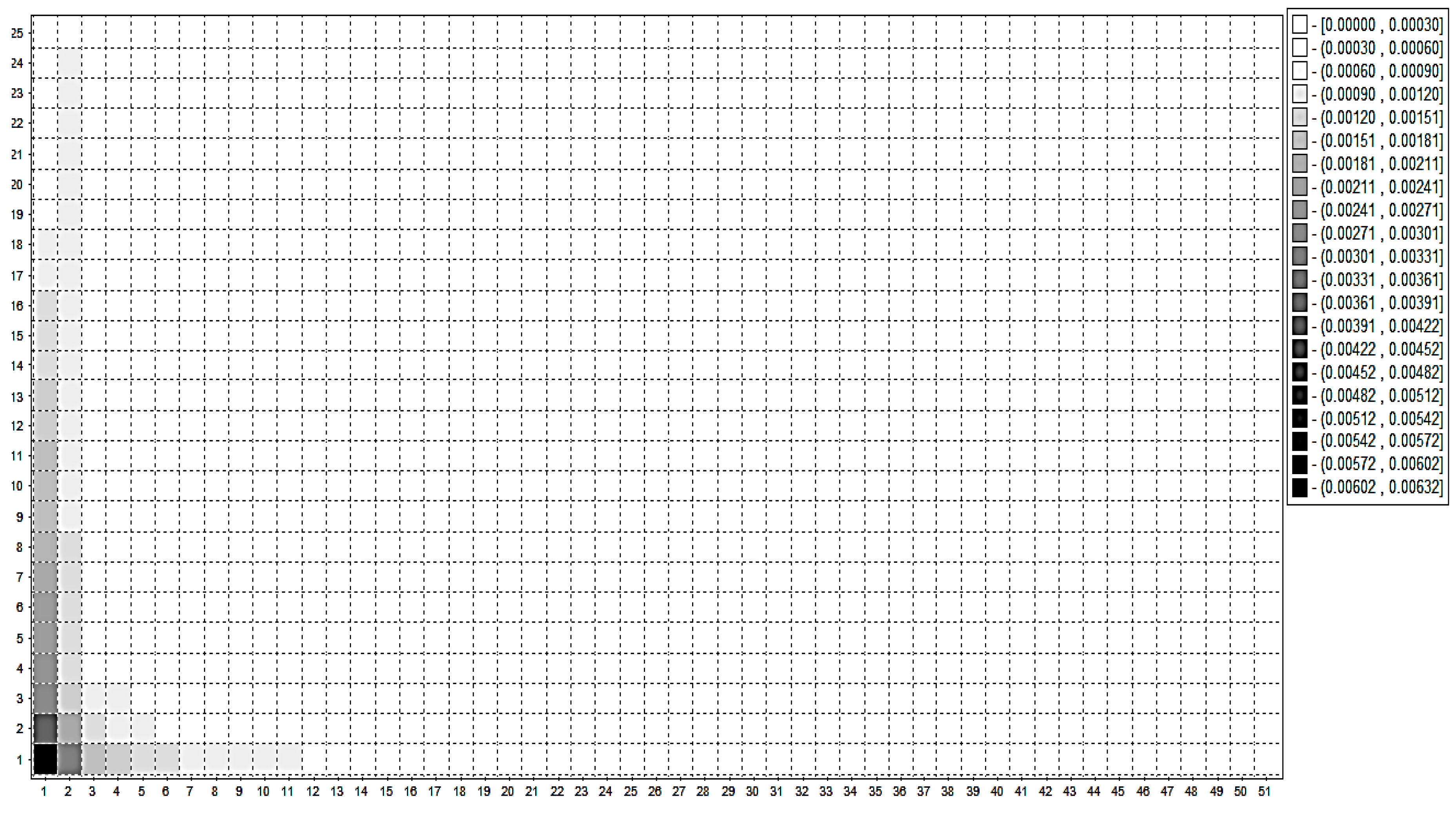
The values of ${\rho }_{12}^{\left(w\right)}$ ensure the concept of separability, however, small absolute values, particularly the ones closed to zero, indicate that the components are well separated. Whereas, big values show that these components are inseparable and therefore they relate to the same components in the SSA decomposition [21,38]. Eventually, projecting the principle components onto the orthogonal matrix of the eigenvectors produces the reconstructed components of our record. Figure 12 shows the moving periodogram matrix of the reconstructed components from which we can see the corresponding eigentriples ordered by their contribution.

Generally, poorly separated components have large correlation while well separated components have small correlation. Groups of correlated series components can be found while looking at the matrix which indicates the w-correlations between elementary reconstructed series. Such information can be used for the consequent grouping. Strongly correlated elementary components should be grouped together in one group. As an important rule, it is recommended that correlated components should not be included into different groups. The matrix of w-correlations between the series components is graphically depicted in absolute magnitude in white-black scale. Importantly, correlations with moduli close to 1 are displayed in black, whereas small correlations are shown in white [58].

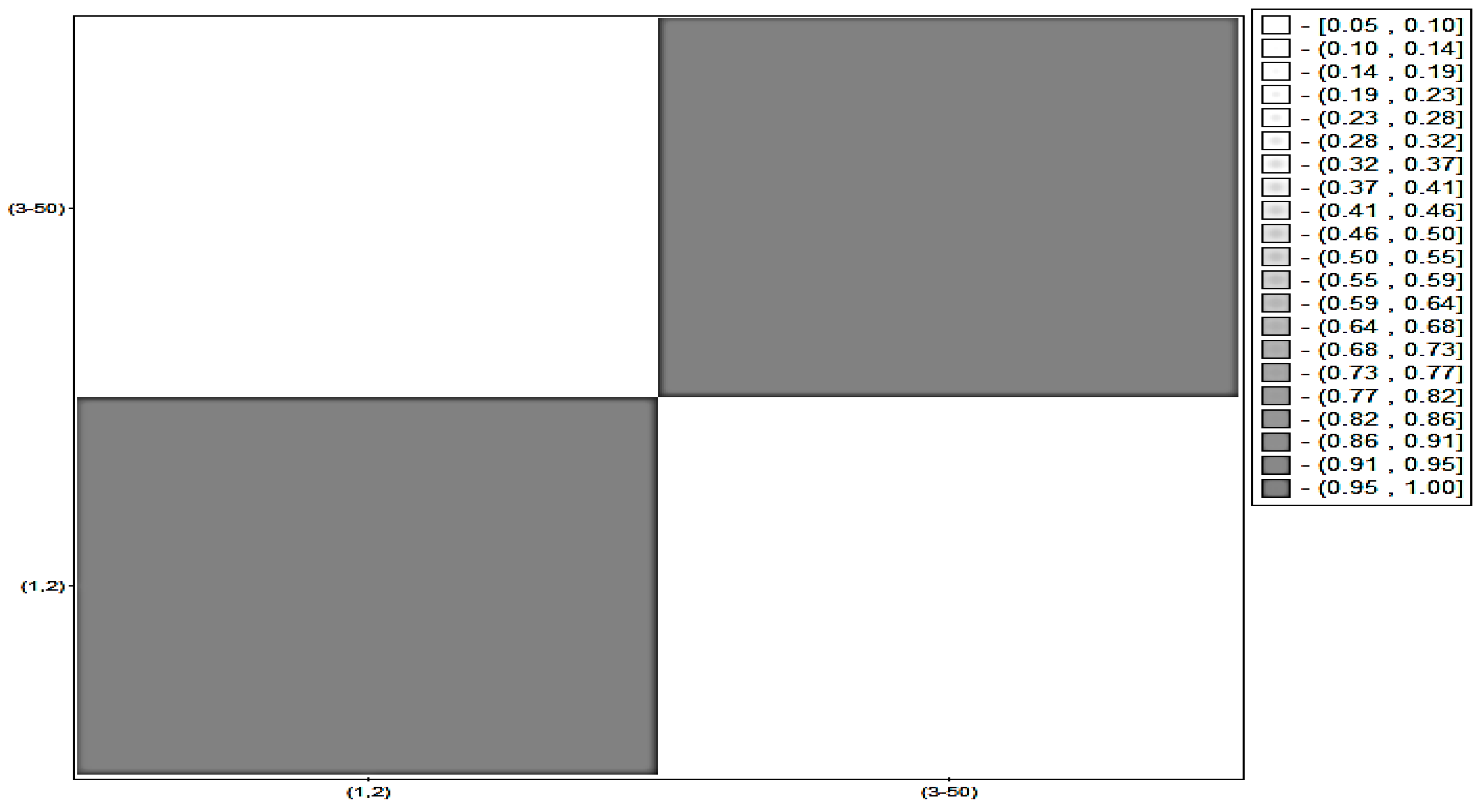
In order to explore the SSA in terms of separability, we considered harmonic and broadband noise, mainly, birds trill and wind noise. These two signals are of different waveform characteristics such as energy, duration and frequency content. Figure 13 illustrates the w-correlations matrix for only the first 50 reconstructed components. The system uses a 20-grade grey scale ranging from white to black which corresponds to the absolute values of correlations from 0 to 1. Components with small correlations are shown in white and indicate well separated components. Whereas big correlation ones shown in black with moduli close to 1.

In terms of the separability, the analysis of this matrix shows that our record has two independent components. Also, we observe that w-correlation shown in white is the correlation between pair eigenvector that represents the noise component and nearly equals to zero. The resultant reconstructed record based on the results approved by the w-correlation is assumed to be noise free and hence; ${\rho }_{(S^{\left(1\right)},S^{\left(2\right)})}^{\left(w\right)}=0$.

Using the eigenvalues spectra helped in efficiently selecting the eigenvectors associated with S1 as a noise free signal and eigenvectors associated with S2 that represent noise. These two groups of eigenvectors are mainly corresponding to different frequency events which eventually lead to their reconstruction. Based on this information; we can consider our dataset is separable with the selection of the first four eigentriples to reconstruct of the original series while the rest is considered as noise.

To assess the effect of noise on a signal, the signal-to-noise ratio (SNR), which is an objective measure, is generally used. It was applied to evaluate the SSA for wind noise reduction in this paper. Results are given in

Table 1. SNR measure applied for evaluating the SSA method for wind noise reduction Measurement cases and difference.

The Objective Measure for Evaluating the Method	Before	After	Difference
SNR in dB	0 dB	9.47 dB	9.47 dB

for comparison.

Before removal the signal to noise ratios are calculated using standard definition. After separation, signal levels and noise levels need to be estimated. The estimated signals to noise ratios are calculated according to:

$$SNR=10\log \frac{{\displaystyle {\sum }_n\stackrel{\wedge }{s}{(n)}^2}}{{\displaystyle {\sum }_n\stackrel{\wedge }{w}{(n)}^2}},$$

(26)

where $\stackrel{\wedge }{s}(n)$ is the estimated signal, $\stackrel{\wedge }{w}(n)$ the estimated noise.

A notable improvement for an average of about 9 dB as it is apparent from Table 1 has been achieved. The result shown in the table is a reported average of a number of cases.

7. Discussion and Conclusions

This paper was set out among our attempts to explore the SSA in microphone wind noise reduction in the context of outdoor sound acquisition for soundscapes and environmental sound monitoring. The plausible findings from the investigation suggest that microphone wind noise and wanted sound, which is birds’ chirps, are separable by the SSA, evidenced by what is indicated by a w-matrix and a 9 dB reduction observed after the SSA de-noising as outlined in this paper.

The only parameter that can be adjusted in the decomposition stage is the window length. This parameter is known to have significant impact on the performance and effectiveness of the algorithm for specific application [59]. The current results were obtained using an optimisation method based on certain important aspects such as the nearly equal singular values. With systematic investigation and more advanced optimisation, the separability might be further improved.

Grouping is another key aspect to consider. The grouping technique reported in this paper is based on the eigentriple for separating the decomposed components after grouping similar components together. The w-correlation method is also involved in our grouping technique. However, very promising results and notable wind noise reduction was achieved. There is always an ambition with more development in the grouping techniques to obtain better results. The experimental investigation and findings indicate the potential of the SSA method as a valid one for wind noise reduction. Indeed, with the SSA, the w-matrix showed that wind noise is separable.

It seems that wind noise has its features clearly separately in the proposed SSA subspaces, indicated by the w-matrix. This suggests that the proposed method is effective and generally robust in separating wind noise. This further suggests that the SSA method should be able to extend to other outdoor audio acquisition or recording. This opens up much more extended applications and impact. Therefore, for future work, more validations with other and bigger datasets will hopefully lead the SSA method to a universal microphone wind noise reduction method and K-Nearest classification systems offer more promise [60].

References

- Glowacz, A.; Glowacz, W.; Glowacz, Z.; Kozik, J. Early fault diagnosis of bearing and stator faults of the single-phase induction motor using acoustic signals. Measurement 2018, 113, 1–9. [Google Scholar] [CrossRef]
- Glowacz, A.; Glowacz, Z. Diagnosis of stator faults of the single-phase induction motor using acoustic signals. Appl. Acoust. 2017, 117, 20–27. [Google Scholar] [CrossRef]
- Jena, D.P.; Panigrahi, S.N. Automatic gear and bearing fault localization using vibration and acoustic signals. Appl. Acoust. 2015, 98, 20–33. [Google Scholar] [CrossRef]
- O’Brien, R.J.; Fontana, J.M.; Ponso, N.; Molisani, L. A pattern recognition system based on acoustic signals for fault detection on composite materials. Eur. J. Mech. A Solids 2017, 64, 1–10. [Google Scholar] [CrossRef]
- Głowacz, A.; Głowacz, Z. Recognition of rotor damages in a DC motor using acoustic signals. Bull. Polish Acad. Sci. Tech. Sci. 2017, 65, 187–194. [Google Scholar] [CrossRef]
- Glowacz, A. Diagnostics of Rotor Damages of Three-Phase Induction Motors Using Acoustic Signals and SMOFS-20-EXPANDED. Arch. Acoust. 2016, 41, 507–515. [Google Scholar] [CrossRef]
- Glowacz, A. Fault diagnostics of acoustic signals of loaded synchronous motor using SMOFS-25-EXPANDED and selected classifiers. Teh. Vjesn. 2016, 23, 1365–1372. [Google Scholar]
- Caesarendra, W.; Kosasih, B.; Tieu, A.K.; Zhu, H.; Moodie, C.A.S.; Zhu, Q. Acoustic emission-based condition monitoring methods: Review and application for low speed slew bearing. Mech. Syst. Signal Process. 2016, 72–73, 134–159. [Google Scholar] [CrossRef]
- Mika, D.; Józwik, J. Normative Measurements of Noise at CNC Machines Work Stations. Adv. Sci. Technol. Res. J. 2016, 10, 138–143. [Google Scholar] [CrossRef]
- Józwik, J. Identification and Monitoring of Noise Sources of CNC Machine Tools by Acoustic Holography Methods. Adv. Sci. Technol. Res. J. 2016, 10, 127–137. [Google Scholar] [CrossRef]
- Fukuda, K. Noise reduction approach for decision tree construction: A case study of knowledge discovery on climate and air pollution. In Proceedings of the 2007 IEEE Symposium on Computational Intelligence and Data Mining, Honolulu, HI, USA, 1 March–5 April 2007. [Google Scholar]
- Yang, B.; Dong, Y.; Yu, C.; Hou, Z. Singular Spectrum Analysis Window Length Selection in Processing Capacitive Captured Biopotential Signals. IEEE Sens. J. 2016, 16, 7183–7193. [Google Scholar] [CrossRef]
- Ma, L.; Milner, B.; Smith, D. Acoustic environment classification. ACM Trans. Speech Lang. Process. 2006, 3, 1–22. [Google Scholar] [CrossRef]
- Chu, S.; Narayanan, S.; Kuo, C. Environmental sound recognition using MP-based features. In Proceedings of the 2008 IEEE International Conference on Acoustics, Speech and Signal Processing, Las Vegas, NV, USA, 31 March–4 April 2008. [Google Scholar]
- Nemer, E.; Leblanc, W. Single-microphone wind noise reduction by adaptive postfiltering. In Proceedings of the Applications of Signal Processing to Audio and Acoustics, New Paltz, NY, USA, 18–21 October 2009; pp. 177–180. [Google Scholar]
- Luzzi, S.; Natale, R.; Mariconte, R. Acoustics for smart cities. In Proceedings of the Annual Conference on Acoustics (AIA-DAGA), Merano, Italy, 18–21 March 2013. [Google Scholar]
- Slabbekoorn, H. Songs of the city: Noise-dependent spectral plasticity in the acoustic phenotype of urban birds. Anim. Behav. 2013, 85, 1089–1099. [Google Scholar] [CrossRef]
- Schmidt, M.N.; Larsen, J.; Hsiao, F.-T. Wind Noise Reduction using Non-Negative Sparse Coding. In Proceedings of the 2007 IEEE Workshop on Machine Learning for Signal Processing, Thessaloniki, Greece, 27–29 August 2007; pp. 431–436. [Google Scholar]
- Schoellhamer, D. H. Singular spectrum analysis for time series with missing data. Geophys. Res. Lett. 2001, 28, 3187–3190. [Google Scholar] [CrossRef]
- King, B.; Atlas, L. Coherent modulation comb filtering for enhancing speech in wind noise. In Proceedings of the 2008 International Workshop on Acoustic Echo and Noise Control (IWAENC 2008), Seattle, WA, USA, 14–17 September 2008. [Google Scholar]
- Harmouche, J.; Fourer, D.; Auger, F.; Borgnat, P.; Flandrin, P. The Sliding Singular Spectrum Analysis: A Data-Driven Non-Stationary Signal Decomposition Tool. IEEE Trans. Signal Process. 2017, 66, 251–263. [Google Scholar] [CrossRef]
- Eldwaik, O.; Li, F.F. Mitigating wind noise in outdoor microphone signals using a singular spectral subspace method. In Proceedings of the Seventh International Conference on Innovative Computing Technology (INTECH 2107), Luton, UK, 16–18 August 2017. [Google Scholar]
- Hassani, H. A Brief Introduction to Singular Spectrum Analysis. 2010. Available online: https://www.researchgate.net/publication/267723014_A_Brief_Introduction_to_Singular_Spectrum_Analysis (accessed on 25 January 2018).
- Jiang, J.; Xie, H. Denoising Nonlinear Time Series Using Singular Spectrum Analysis and Fuzzy Entropy Denoising Nonlinear Time Series Using Singular Spectrum Analysis and Fuzzy Entropy. Chin. Phys. Lett. 2016, 33. [Google Scholar] [CrossRef]
- Qiao, T.; Ren, J.; Wang, Z.; Zabalza, J.; Sun, M.; Zhao, H.; Li, S.; Benediktsson, J.A.; Dai, Q.; Marshall, S. Effective Denoising and Classification of Hyperspectral Images Using Curvelet Transform and Singular Spectrum Analysis. IEEE Trans. Geosci. Remote Sens. 2017, 55, 119–133. [Google Scholar] [CrossRef]
- Hassani, H.; Zokaei, M.; von Rosen, D.; Amiri, S. Does noise reduction matter for curve fitting in growth curve models? Comput. Methods 2009, 96, 173–181. [Google Scholar] [CrossRef] [PubMed]
- Golyandina, N.; Shlemov, A. Semi-nonparametric singular spectrum analysis with projection. Stat. Interface 2015, 10, 47–57. [Google Scholar] [CrossRef]
- Hassani, H.; Soofi, A.; Zhigljavsky, A. Predicting daily exchange rate with singular spectrum analysis. Nonlinear Anal. Real World Appl. 2010, 11, 2023–2034. [Google Scholar] [CrossRef]
- Xu, X.; Zhao, M.; Lin, J. Detecting weak position fluctuations from encoder signal using singular spectrum analysis. ISA Trans. 2017, 71, 440–447. [Google Scholar] [CrossRef] [PubMed]
- García Plaza, E.; Núñez López, P.J. Surface roughness monitoring by singular spectrum analysis of vibration signals. Mech. Syst. Signal Process. 2017, 84, 516–530. [Google Scholar] [CrossRef]
- Claessen, D.; Groth, A. A Beginner’s Guide to SSA. 2002. Available online: http://environnement.ens.fr/IMG/file/DavidPDF/SSA_beginners_guide_v9.pdf (accessed on 25 January 2018).
- Moskvina, V.; Zhigljavsky, A. An Algorithm Based on Singular Spectrum Analysis for Change-Point Detection. Commun. Stat. Simul. Comput. 2003, 32, 319–352. [Google Scholar] [CrossRef]
- Elsner, J.B.; Tsonis, A.A. Singular Spectrum Analysis: A New Tool in Time Series Analysis; Springer: New York, NY, USA, 2013. [Google Scholar]
- Ghodsi, M.; Hassani, H.; Sanei, S.; Hicks, Y. The use of noise information for detection of temporomandibular disorder. Biomed. Signal Process. 2009, 4, 79–85. [Google Scholar] [CrossRef]
- Hu, H.; Guo, S.; Liu, R.; Wang, P. An adaptive singular spectrum analysis method for extracting brain rhythms of electroencephalography. PeerJ 2017, 5, e3474. [Google Scholar] [CrossRef] [PubMed]
- Lakshmi, K.; Rao, A.R.M.; Gopalakrishnan, N. Singular spectrum analysis combined with ARMAX model for structural damage detection. Struct. Control Heal. Monit. 2017, 24, 1–21. [Google Scholar] [CrossRef]
- Alonso, F.; del Castillo, J.; Pintado, P. Application of singular spectrum analysis to the smoothing of raw kinematic signals. J. Biomech. 2005, 38, 1085–1092. [Google Scholar] [CrossRef] [PubMed]
- Traore, O.I.; Pantera, L.; Favretto-Cristini, N.; Cristini, P.; Viguier-Pla, S.; Vieu, P. Structure analysis and denoising using Singular Spectrum Analysis: Application to acoustic emission signals from nuclear safety experiments. Measurement 2017, 104, 78–88. [Google Scholar] [CrossRef]
- Hassani, H.; Heravi, S.; Zhigljavsky, A. Forecasting European industrial production with singular spectrum analysis. Int. J. Forecast. 2009, 25, 103–118. [Google Scholar] [CrossRef]
- Chu, M.T.; Lin, M.M.; Wang, L. A study of singular spectrum analysis with global optimization techniques. J. Glob. Optim. 2013, 60, 551–574. [Google Scholar] [CrossRef]
- Golyandina, N.; Nekrutkin, V.; Zhigljavsky, A. Analysis of Time Series Structure: Ssa and Related Techniques; CRC Press: Boca Raton, FL, USA, 2001. [Google Scholar]
- Launonen, I.; Holmström, L. Multivariate posterior singular spectrum analysis. Stat. Methods Appl. 2017, 26, 361–382. [Google Scholar] [CrossRef]
- Golyandina, N.E.; Lomtev, M.A. Improvement of separability of time series in singular spectrum analysis using the method of independent component analysis. Vestn. St. Petersbg Univ. Math. 2016, 49, 9–17. [Google Scholar] [CrossRef]
- Hassani, H. Singular spectrum analysis: Methodology and comparison. J. Data Sci. 2007, 5, 239–257. [Google Scholar]
- Clifford, G.D. Singular Value Decomposition & Independent Component Analysis for Blind Source Separation. Biomed. Signal Image Process. 2005, 44, 489–499. [Google Scholar]
- Ghil, M.; Allen, M.R.; Dettinger, M.D.; Ide, K.; Kondrashov, D.; Mann, M.E.; Robertson, A.W.; Saunders, A.; Tian, Y.; Varadi, F.; et al. Advanced spectral methods for climatic time series. Rev. Geophys. 2002, 40, 1003. [Google Scholar] [CrossRef]
- Patterson, K.; Hassani, H.; Heravi, S. Multivariate singular spectrum analysis for forecasting revisions to real-time data. J. Appl. 2011, 38. [Google Scholar] [CrossRef]
- Maddirala, A.; Shaik, R.A. Removal of EOG Artifacts from Single Channel EEG Signals using Combined Singular Spectrum Analysis and Adaptive Noise Canceler. IEEE Sens. J. 2016, 16, 8279–8287. [Google Scholar] [CrossRef]
- Golyandina, N.; Korobeynikov, A. Basic singular spectrum analysis and forecasting with R. Comput. Stat. Data Anal. 2014, 71, 934–954. [Google Scholar] [CrossRef]
- Vautard, R.; Ghil, M. Singular spectrum analysis in nonlinear dynamics, with applications to paleoclimatic time series. Physica D 1989, 35, 395–424. [Google Scholar] [CrossRef]
- Moore, J.; Glaciology, A. Singular spectrum analysis and envelope detection: Methods of enhancing the utility of ground-penetrating radar data. J. Glaciol. 2006, 52, 159–163. [Google Scholar] [CrossRef]
- Vautard, R.; Ghil, M. Interdecadal oscillations and the warming trend in global temperature time series. Nature 1991, 350, 324–327. [Google Scholar]
- Alexandrov, T. A Method of Trend Extraction Using Singular Spectrum Analysis. 2009. arXiv.org e-print archive. Available online: https://arxiv.org/abs/0804.3367 (accessed on 25 January 2018).
- Rodrigues, P.C.; Mahmoudvand, R. The benefits of multivariate singular spectrum analysis over the univariate version. J. Frankl. Inst. 2017, 355, 544–564. [Google Scholar] [CrossRef]
- Rukhin, A.L. Analysis of Time Series Structure SSA and Related Techniques. Technometrics 2002, 44, 290. [Google Scholar] [CrossRef]
- Hassani, H.; Mahmoudvand, R. Multivariate Singular Spectrum Analysis: A General View and New Vector Forecasting Approach. Int. J. Energy Stat. 2013, 1, 55–83. [Google Scholar] [CrossRef]
- Hansen, B.; Noguchi, K. Improved short-term point and interval forecasts of the daily maximum tropospheric ozone levels via singular spectrum analysis. Environmetrics 2017, 28, e2479. [Google Scholar] [CrossRef]
- Golyandina, N.; Shlemov, A. Variations of singular spectrum analysis for separability improvement: Non-orthogonal decompositions of time series. Stat. Interface 2015, 8, 277–294. [Google Scholar] [CrossRef]
- Pan, X.; Sagan, H. Digital image clustering algorithm based on multi-agent center optimization. J. Digit. Inf. Manag. 2016, 14, 8–14. [Google Scholar]
- Secco, E.L.; Deters, C.; Wurdemann, H.A.; Lam, H.K.; Seneviratne, L.; Althoefer, K. A K-Nearest Clamping Force Classifier for Bolt Tightening of Wind Turbine Hubs. J. Intell. Comput. 2016, 7, 18–30. [Google Scholar]
Figure 1.
The two complementary stages of the SSA method.
Figure 2.
A descriptive process of the SSA method.
Figure 3.
Main aspects in the SSA method.
Figure 4.
Representation of a given time series when considering for example a window length m = 4 to construct the trajectory matrix.
Figure 5.
A flow chart of the experimental procedure.
Figure 6.
Window length optimisation using seven different values of the frame length.
Figure 7.
Singular spectra of clean record of birds’ chirps and a noisy one with wind noise added.
Figure 8.
The leading four principle components used for grouping and reconstruction and the record of birds’ chirps with additive wind noise: (a) Reconstruction with the first two leading pairs of the principle components; (b) Reconstruction with the third and fourth principle components pairs.
Figure 9.
Reconstructed series vs original noisy signal and residual series.
Figure 10.
The de-noised record was separated by retaining only the leading two pairs of the eigenvalues.
Figure 11.
A combination of our signals used in the experiments: (a) Noisy record (birds’ chirps and wind noise); (b) Clean record of birds’ chirps.
Figure 12.
Moving periodogram matrix of reconstructed components.
Figure 13.
Matrix of w-correlations of the selected 50 eigenvectors of the SVD of the trajectory matrix.