1. Introduction
Technology is defined as theoretical and practical knowledge, skills and artifacts exploited to develop products, production and delivery systems [
1]. Due to the great influence of technology capability on the achievement of a firm’s competitive advantage [
2] and the growth of industrial and academic interest in how to manage technology more effectively [
3], studies on this issue have increased through recent years and researchers interpret technology as a strategic phenomenon [
4]. Management of technology (hereafter MOT), as a management system, concerns planning, directing, controlling and coordinating technological capabilities and comprises five main processes/functions, namely identification, selection, acquisition, protection and exploitation [
5].
Due to their large effect on firm competitiveness and the considerable cost and risk imposed on the company, some MOT processes are challenging. In such cases, technology selection (henceforth TS) becomes one of the most challenging processes of MOT [
6], and should be approached strategically [
7]. Linking strategy to technology has been an issue in recent years, due to a novel model developed by the Stanford Research Institute (SRI) called “technology portfolio analysis”. Later, this model was investigated by Morin [
8] (see
Figure 1). On the basis of the SRI model, potential technologies that seem attractive, but which the firm lacks the sufficient capabilities to reach, require further inspection.
In this research, a hybrid best–worst, multi-criteria decision-making model (BWM) and total area based on orthogonal vectors (TAOV) methodology are used to prioritize and select the best technologies in the chosen quadrant. Furthermore, a multi-objective decision model (MODM) is implemented to refine the model and illustrate the scheduling program for implementing the selected projects.
Technology selection is the process of choosing the “best” technology alternatives (in terms of technology area, technology option and/or R&D project) from a set of available candidates [
9]. Regarding the selection of the best technology option, it is notable that differences between a firm’s (internal and external) context and objectives, produces different technological requirements; therefore, the “best” technology option becomes quite specific.
Regarding the fact that technology selection (TS) is challenging and results in strategic preferences, two points of view are considerable. From the external context, the dynamics of market and industry [
10], pace of technological changes, complexity of new technologies and shrinkage of product life cycles are some determinant factors making TS highly challenging and strategic. On the other hand, from an internal viewpoint, difficulties in TS process are specific and consist of many organizational obstacles. TS requires considering different characteristics of each technology option, compromising their relevancy to organizational goals, risk and suitability with a firm’s capabilities. Moreover, technology options should be selected considering other key decisions regarding their acquisition mode, development possibilities and introduction scheduling [
7].
Studies have introduced many methods to aid managers and decision-makers in evaluating and selecting appropriate technology [
11], such as the scoring method—e.g., Coldrick et al. [
12]—or multi-attribute utility theory—e.g., Duarte and Reis [
13]. Supply chain technologies were tested recently as Shen et al. [
14] proposed a multi criteria decision making and principle component analysis (MCDM-PCA) hybrid model for technology selection while Farooq O’Brien [
15] considered the risks of TS by examining a manufacturing company. Moreover, Sahin and Yip [
16] investigated TS for shipping methods based on an improved Gaussian fuzzy analytical hierarchical process (AHP) model, besides Xia et al. [
17] studied sustainability TS in a considered supply chain.
A case of photovoltaic technology selection has been presented recently by Van De Kaa et al. [
18], who implemented a fuzzy and crisp MCDM approach to evaluate five technologies. Some of the selecting methods simply analyze candidate projects independently (e.g., [
19]), while correlations between projects may cause an unselected project to be chosen (e.g., [
20]). Hence, recently there has been an increasing interest in implementing the portfolio selection method for selecting technology options. In this context, Roussel et al. [
21] argued that for the sake of effective R&D management, a defined firm needs to take a comprehensive view of all R&D activities. Portfolio management as one of the most important senior management functions [
22] for selecting R&D project is defined as a dynamic decision-making process [
23].
The remainder of this paper is divided as follows. A thorough review of the recent developed MCDM method—BWM—is proposed, furthermore, the TAOV methodology is discussed and a real-world problem related to technology selection is resolved. The authors present a binary model to schedule the project option implementation procedure. Eventually, some suggestions for future research are provided in the conclusion.
2. Best–Worst Methodology (BWM)
Continuous and discrete MCDM problems have been discussed on many subjects using different techniques in the last decade. The most prevalent of these are Complex Proportional Assessment (COPRAS) [
24], Elimination and Choice Expressing Reality (ELECTRE) [
25], Analytic Hierarchy Process (AHP) [
26], VIseKriterijumska OptimizancijaI Kompromisno Resenje (VIKOR) [
27], and many other methods such as Preference Ranking Organization Method for Enrichment Evaluations (PROMETHEE), Step-wise Weight Assessment Ratio Analysis (SWARA) or Technique for Order of Preference by Similarity to Ideal Solution (TOPSIS). Researchers can refer to [
28] for more information about MCDM methods and a comparison between them.
Rezaei [
29] developed BWM as a new MCDM methodology, then proposed a supportive article to introduce some of its properties and a linear model [
30]. Scholars have used this method since then to identify enablers of technological innovation in Micro, Small and Medium Enterprises (MSMEs) in India [
31], utilizing this method for the supplier selection life cycle [
32], to evaluate the external forces affecting the sustainability of the oil and gas supply chain [
33], or even wielding this tool in order to develop a roadmap to overcome barriers to energy efficiency in buildings [
34]. Recently, intuitionistic fuzzy multiplicative BWM has been proposed by [
35] to extend the method’s use to uncertain circumstances.
As the name best–worst method conspicuously indicates, this MCDM tool is based on the comparison of desired criteria. Rezaei [
29] believes that comparing two random criteria is time intensive and ineligible as the vector becomes bigger and the process gets longer. Therefore, the best and worst criteria are chosen among the proposed criterion suggested by decision-makers and the whole purpose is to find the optimal weights and consistency radio (CR) through an optimization model constructed using the comparison between the best criteria over others and vice versa.
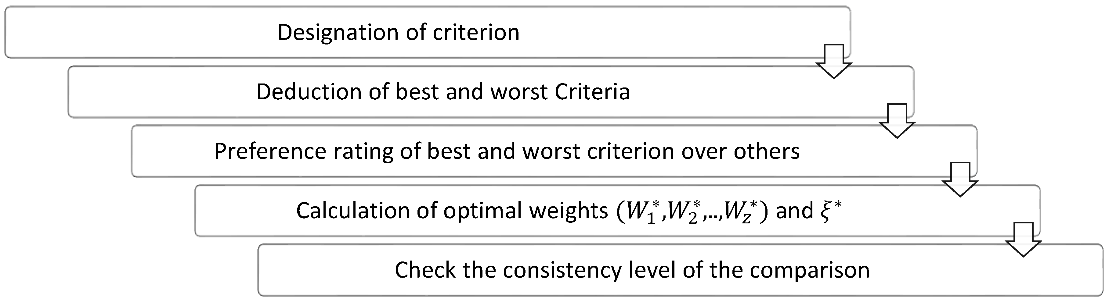
Figure 2 indicates the BWM process as a system and briefly sets out the steps in the rest of this section based on [
29,
31,
32].
Step 1: Designation of criterion.
Scholars combine previous works and expert opinions on a subject to find out a set of
criteria which would be:
Step 2: Deduction of best and worst criteria.
The best criterion is interpreted as the most illustrious and glorious among the rest of the criterion, whereas the least valued criteria is labeled as the worst criteria. The identification is based on decision-maker opinions and the values of the criteria are not considered at this stage.
Step 3: Preference rating of best and worst criterion over others.
This step can be broken into two sub-steps where the decision-makers indicate the preference of the best criteria
over the rest of criterion
(i.e.,
) in a first step and then investigate the preference of all criterion
over the worst criteria
(i.e.,
). In order to do so, a number between 1 and 9 is allocated for each pair.
Step 4: Determine the optimal weights.
The optimal weights of the criterion are deduced by the maximization of absolute differences
for all
that should be minimized, which would be translated as follows:
The aforementioned formula is commuted into a linear programming formulation as below:
Solving Formula (5) results in distinctive results consisting of the optimal weights and a consistency ratio of the comparison system ().
Step 5: Consistency level check.
Acquiring the weights of each criteria using (5) leads to scrutinizing the consistency level of the comparisons. CR ( is the key number in this collation, as the value gets closer to 0, the comparison system provided by decision-maker becomes more consistent.
For the evaluation of weights using BWM, the TAOV method is utilized to rate the criterion as a new MCDM model. The described method in next section is based on Hajiagha et al. [
36].
3. Total Area Based on Orthogonal Vectors (TAOV)
The foundation of this model consists of the three stages of initialization, orthogonalization and comparison as a whole. The rest of this section details the method in three phases.
Phase 1. Initialization
Decision-makers nominate a number of alternatives
and define determinant criterion
based on those alternatives. Heeding the gathered information, the decision matrix is constructed as below:
Considering the fact that
represents the behavior of alternative
over criteria
, the weight vector of alternatives
is obtained using classic methods such as pairwise comparison [
37] or implementing new methods like SWARA [
38]. In this paper, BWM was used to construct the weight vector.
Like any other MCDM technique, the aforementioned decision matrix (6) should be normalized. The selected criterion is classified into two groups of beneficial (
) and cost criterion (
). Designation as a beneficial criteria indicates that the higher value is worth more, whereas the cost criterion is better kept low in the decision-making process. The normalization procedure is illustrated as follows:
Thereafter the normalized matrix is fabricated as:
Having obtained the weighted vector from BWM and the normalized matrix, the weighted-normalized matrix (
) is obtained as below. Note that
for each element.
Phase 2. Orthogonalization
This method dictates that in order to avoid correlation between any two columns of the weighted and normalized matrix, it is critical to transform current criteria vectors (i.e.,
to orthogonal vectors
. To achieve this, applying principal component analysis (PCA) to the
matrix has been suggested (10). Application of this tool results in a linear combination of vectors called principal components that are independent. Jolliffe [
39] describes each principal component,
, as a set of weighted-normalized vectors
. In other words, the transformation process is shown as below:
Principle component analysis (PCA) uses the weights in
for the transformation procedure in tools like statistical package for social sciences (SPSS) package to formulate the orthogonal decision matrix as below:
Considering each
component decomposed to
, it consists of the coefficients of the variables in the
j-th component (i.e., (
). Deploying Euclidean distance function, the distance between the different components are calculated as below:
Phase 3. Comparison
The total area (TA) of alternative is calculated to indicate the performance of alternatives on any criteria as follows:
The attractiveness of alternatives is computed using the normalized total area (NTA) as:
4. Proposed Approach
In this section, four phases of our proposed approach are discussed to provide better understanding of the approach and to introduce the basic elements performed in this research.
Phase I: Identification
The basic goal of this research was to investigate the importance of integration in choosing the best projects for high-tech businesses such as the proposed case; therefore, the case of an Iranian IT company (Tehran, Iran) was picked to probe the available technology options. The company assisted scholars with a list of 23 technology options, the options were then plotted in form of a capability–attractiveness portfolio to distinguish the attractive projects that lack sufficient capabilities. Researchers were asked to investigate how attractive these projects are, in order to examine the feasibility of implementing the most attractive projects in a period of three years.
Phase II: Weighting
The importance of using decision-making tools for contemporary problems is strong and scholars use classic and new methods in both certain and uncertain cases to create a better picture of these tools. During recent years, some new methods have emerged that seem to be more practical and easier to use. The BWM method is an accurate tool that helps scholars assess the weight of the criteria comfortably. Considering the pairwise comparison table (
Appendix A,
Table A1)
and
vectors were formed in order to compare the criteria to the best and worst criteria. Subsequently, using Formula (5), a simple problem was solved using the LINGO (software package for linear programming, integer programming, nonlinear programming, stochastic programming and global optimization) program to obtain the weights of each criterion.
Phase III: Selecting
Moving on into this phase, another new MCDM method called TAOV—which has been successfully compared to other classic methods before by [
36]—was utilized to sort out the selected projects based on the weights obtained from the last phase. The normalized matrix was formulated using the weights obtained from BWM. According to Formula (10), the weighted normalized matrix is structured. Subsequently, using the SPSS package, a principal component analysis (PCA) on the
matrix was performed successfully in order to construct the
matrix (Formula (11)). Scholars computed the distance between different components (Formulas (13) and (14)) and compared the results (Formula (15)). Eventually, the final scores obtained from TAOV method are summarized.
Phase IV: Scheduling
Although the three components of risk, time and cost were considered in the prioritizing session, there are many other points that need to be noted in the decision-making procedure. In order to make this case narrower, the company was asked to consider a time limitation of three years. Moreover, they need to manage a finite amount of money allocated each year to the R&D department and to make sure that running these projects will not conflict with each other as some of them need more resources and some need higher consideration to be implemented successfully. Furthermore, another obstacle is the number of projects the company can handle each year. A complete illustration of our proposed formulation is depicted below as:
Table 1 introduces the symbols used in the mentioned model.
To conclude this section,
Figure 3 illustrates a scheme of the hybrid BWM-TAOV approach used in this paper.
5. Case Study
The case was chosen of one of the branded Iranian IT companies working as a solution provider for businesses and governmental organizations. Owing to secrecy issues, the company’s name is not mentioned. In order to gain more value from the market, the strategic planning department of the company formulated growth-oriented strategies and objectives. The technical nature of the company raised many technological requirements that had to be addressed by company’s technology strategy. Responding to technological requirements of the company, twenty-three technology options (TOs) were identified by company’s CTO (Chief Technology Officer) consulting with key functional managers. Among them, nine TOs were existing and fourteen TOs were new to the firm.
Due to the shortage of resources and capabilities, the firm needed to assess alternative TOs before selection. Evaluating technology attractiveness (TEA) and auditing technological capability (TC) are two major parts of a technology assessment process. Based on Jolly [
40], nine criteria for TEA and TC were chosen (
Table 2).
For the purpose of the technology assessment, a panel of 15 experts consisting of the company’s CTO, key middle managers and some technical consultants was formed to score each TO upon a questionnaire provided in
Appendix A,
Table A2. The average of their scores for each TO is illustrated in
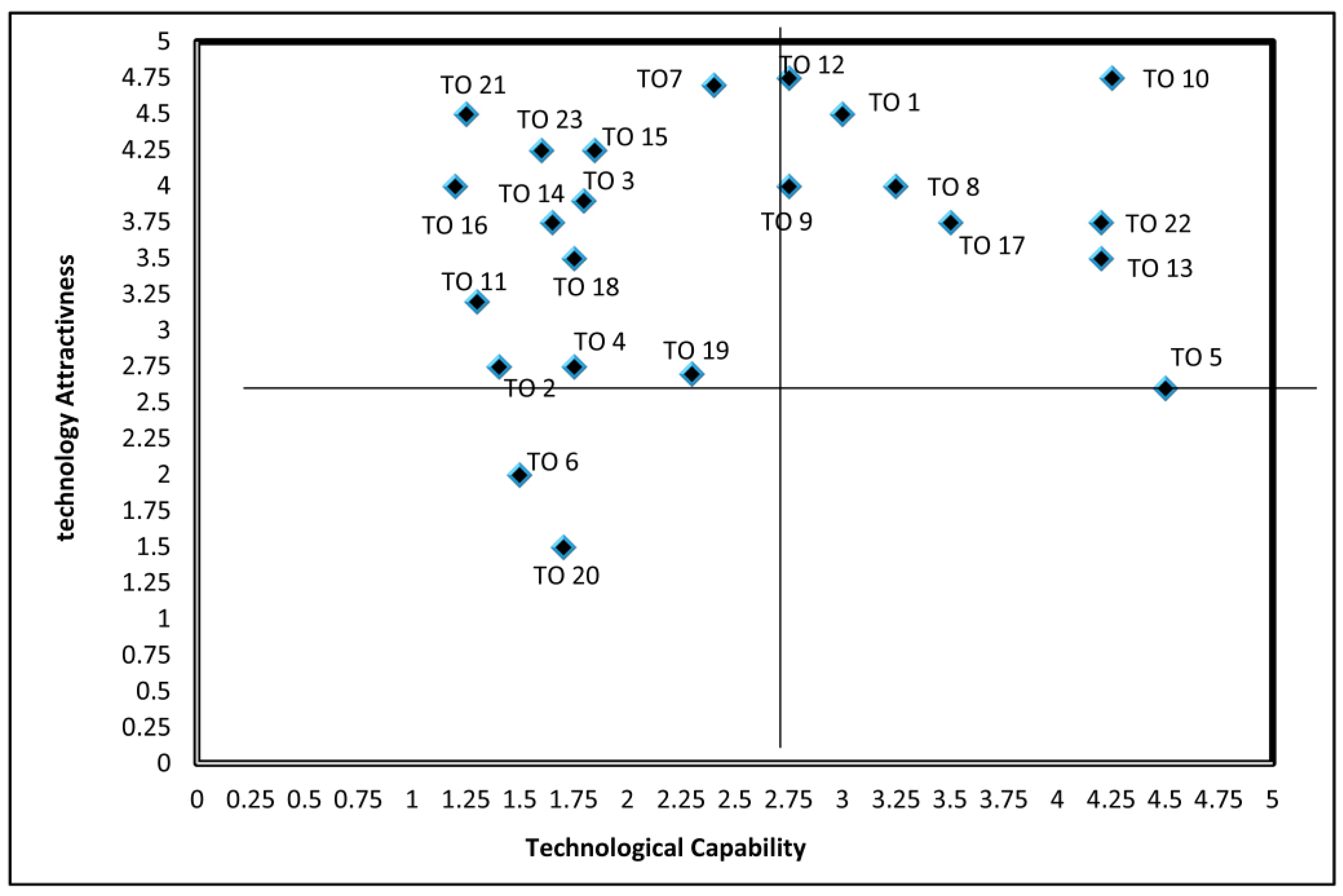
Table 3. The experts have evaluated the technology options based on two basic factors (i.e., technology capability and technology attractiveness). The implemented approach employed in this article is going to investigate the problem targeting multi-objective criterion and structural factors like budget, time and other constraints to construct and solve a zero or one linear programming (ZOLP) problem based on the aforementioned constraints. Furthermore, the proposed model aims to guarantee that the company makes the most profit as well as determining the optimal time to start each project. The technology assessment results are shown in
Table 3 and are plotted in a capability–attractiveness portfolio (
Figure 4).
Since there are many new technologies that have the potential of achieving the technological requirements of firms, the top-left zone of the capability–attractiveness portfolio consists of a considerable number of TOs that should be evaluated in the final selection. Acquiring each TO in the top-left zone of the portfolio imposes different levels of risk (the risk that a company burdens TO functionality and performance over time), cost (estimated costs of developing a technology) and different acquisition times (the amount of time a technology takes to be developed). Though the three relevant criteria to each TO located in the top-left zone of the portfolio were assessed from the experts’ opinions, based on a company’s capabilities, assessments (Human Resource and Research and Development) and Iran’s potential capability for developing a technology. Technology options were then converted using a Likert scale (a pair-wise scale is provided in the
Appendix A). The final results are shown in
Table 4 in terms of high (H), medium (M) and low (L) scores.
Time consuming projects destroy the efforts and resources of firms (worst criteria), although a positive side of risk-taking is profit and firms gain profit by implementing hazardous projects (best criteria). Considering the best and worst criteria in the BWM, the method suggests comparing these criteria to others. Therefore, after a brainstorming session where
and
vectors where suggested as
and
the weights were then obtained by solving (Formula (5)) as
. The applied model is demonstrated as below:
In order to use TAOV method, the decision matrix was normalized and is shown in
Table 5.
Table 6 illustrates the effect of weights on the normalized matrix by multiplying the acquired weight vector from BWM on the decision making matrix.
Subsequently, principle component analysis was implemented on the matrix to attain the square matrix shown below in
Table 7.
The
matrix is formed by multiplying the PCA matrix by the weighted–normalized matrix; the result is shown in
Table 8.
The final step of TAOV is finding the total area of alternatives using (13) and (14). Following that step, the normalized total area is computed to lead scholars in finding the final ranking of alternatives. The last step is summarized in
Table 9.
The firm provided us with a list of the estimated financial budget needed to run each project successfully. The list is shown in
Table 10.
The firm has limited technical and human resources to run a certain number of projects each year. The firm suggested starting five projects each year; therefore, the following constraint is formulated for the restriction in the number of projects for next three years.
Financial support is the main driver of R&D department annual project scheduling, whereas the scanty allocation of funds to R&D departments leads them to the production of commoditized products which is risky for high-tech companies. Therefore, the firm has assigned a fixed budget of 35 million dollars for each year and the R&D department needs to manage this money to choose the best projects each year. The formulation in (17) depicts the role of financial issues in the decision-making process.
Project integration is a matter of resource management in firms. Among these projects there is a close relationship between some of them; therefore, the R&D team has arranged these projects in a four-stage cluster to make sure they are managing their resources under optimal conditions. Moreover, these projects are supposed to be performed in the exact period of three years to stay in competition with other high-tech competitors. The grouping and formulation brief is shown as below.
The goal is to maximize the firm’s profit by choosing the most valuable project in the exact time, the objective function contains the sum of the scores obtained from the BWM-TAOV approach.
Solving the problem (20) using LINGO dissociates the projects from each other and allocates them to certain years due to the constraints and budget limitations.
Table 11 illustrates the obtained results.
The results indicated that the project implementation program should be organized as in
Table 11. As illustrated, project 2, 4, 8, 12 should begin in the first year; projects 1, 6, 9 should begin at the beginning of the second year; and finally projects 3, 5, 7, 10, 11 should be considered for the third year of the program.
It is obvious that the firm has the opportunity to focus on process, human resource and technological development in the first years and postpone the pressure of projects to the last year. On the other hand, utilizing the first and third most valuable projects in the first year is a confidence insurance for the firm to keep working on the rest of the projects for the next two years.
6. Conclusions
Project integration and budget considerations are simultaneously two of the most important aspects that managers need to plan in R&D departments. Although this has been rarely investigated by scholars, this research examined the importance of integration and budget in a limited period of time for the most attractive technology options using a new novel BWM-TAOV approach. The selection process for development projects, ranking them and eventually presenting a scheduling scheme to perform the projects on the basis of a binary model including multiple criteria and constraints were considered in the suggested approach, as these were the primary objectives of this article. The integration of ZOLP and MCDM techniques specifies more accurate and persistent answers. Though the lack of research in this field using hybrid approaches hinders the authors from compare the findings to any other articles.
Scholars can extend this work by adding more constraints and solving a multi-objective problem. Moreover, the technology options or any other variables can be probed in the interval mode for more extant results. Furthermore, considering qualitative criteria in the designed decision-making process, performing new uncertainty approaches such as interval valued intuitionistic fuzzy number (IVIF), interval valued fuzzy number (IVF) and hesitant fuzzy linguistic term sets (HFLTS) is recommended. The weighting technique (BWM) and ranking model (TAOV) operated in this research are almost the newest available methods; nonetheless, other possible approaches are applicable in our advised approach.

 ,
, 


