FPGA-Based Implementation of a Multilayer Perceptron Suitable for Chaotic Time Series Prediction


 ,
,
Abstract
:1. Introduction
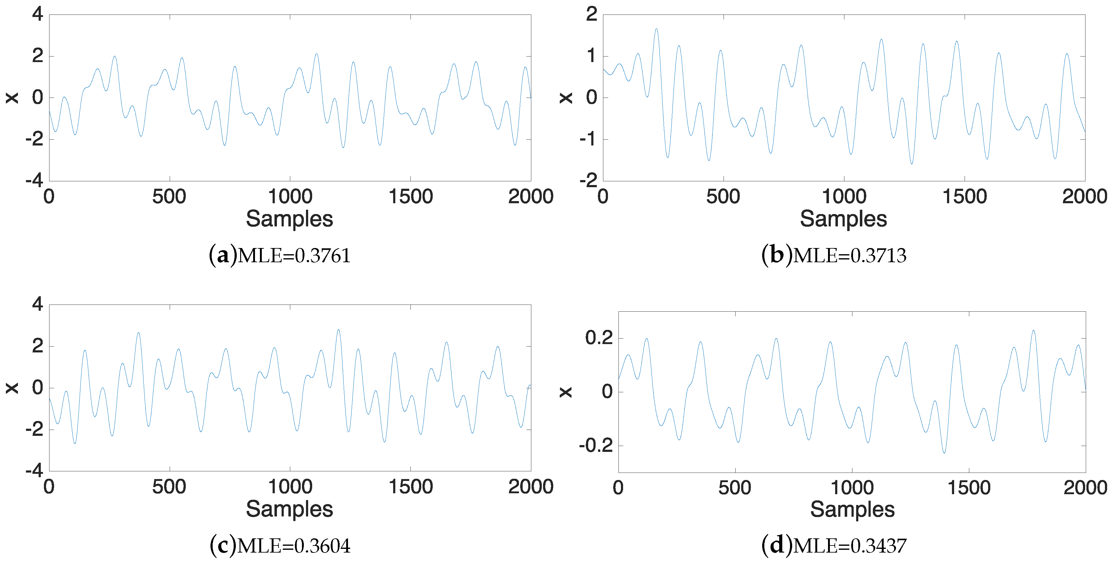
2. Generating Chaotic Time Series
3. Chaotic Time Series Prediction Techniques
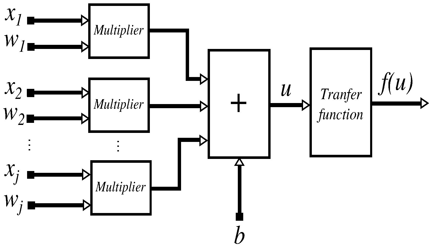
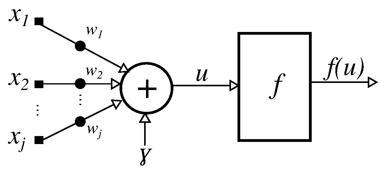
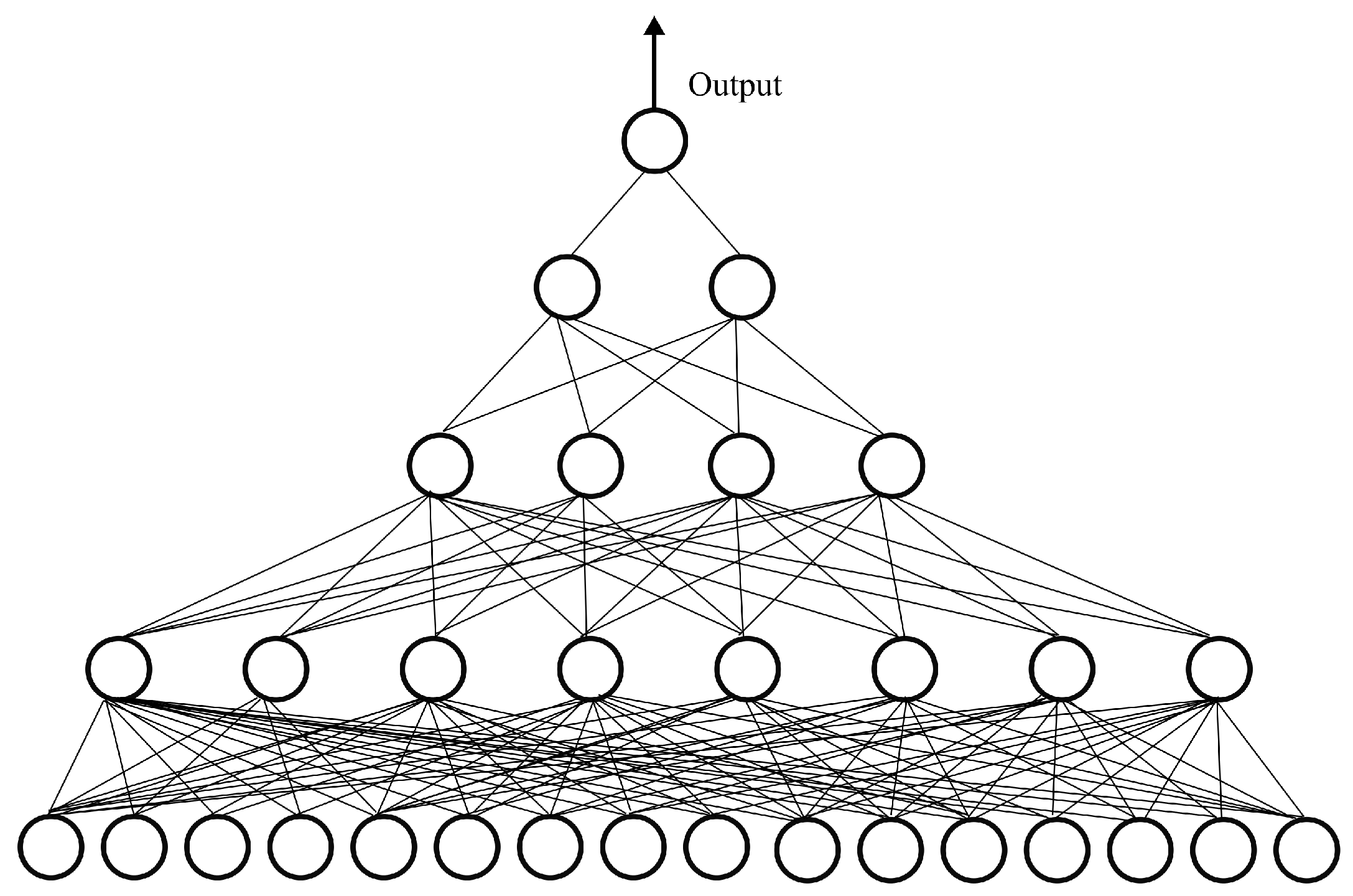
3.1. Artificial Neural Networks
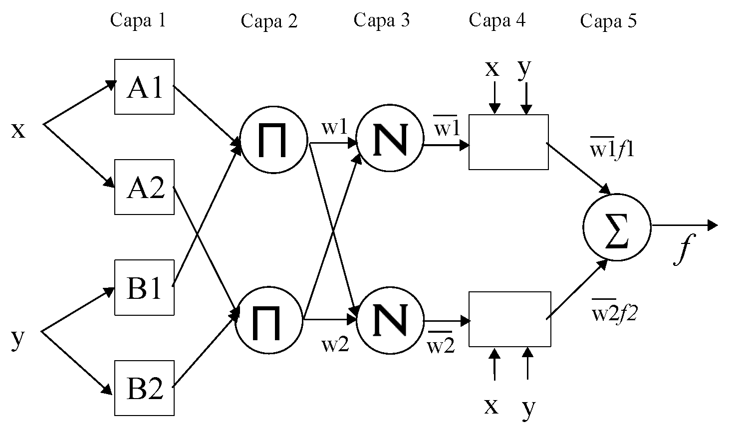
3.2. Adaptive Neuro-Fuzzy Inference System
- Layer 1 contains input nodes passing external signals to the next layer.
- Layer 2 performs the parameter adjustment of the input membership function.
- Layers 3 and 4 perform fuzzy operations.
- Layers 5 and 6 weight and provide the output of the system.
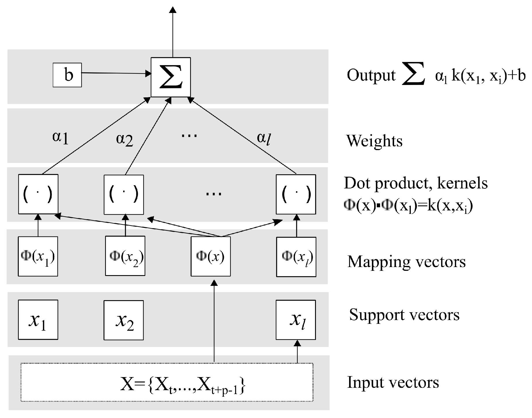
3.3. Support Vector Machine
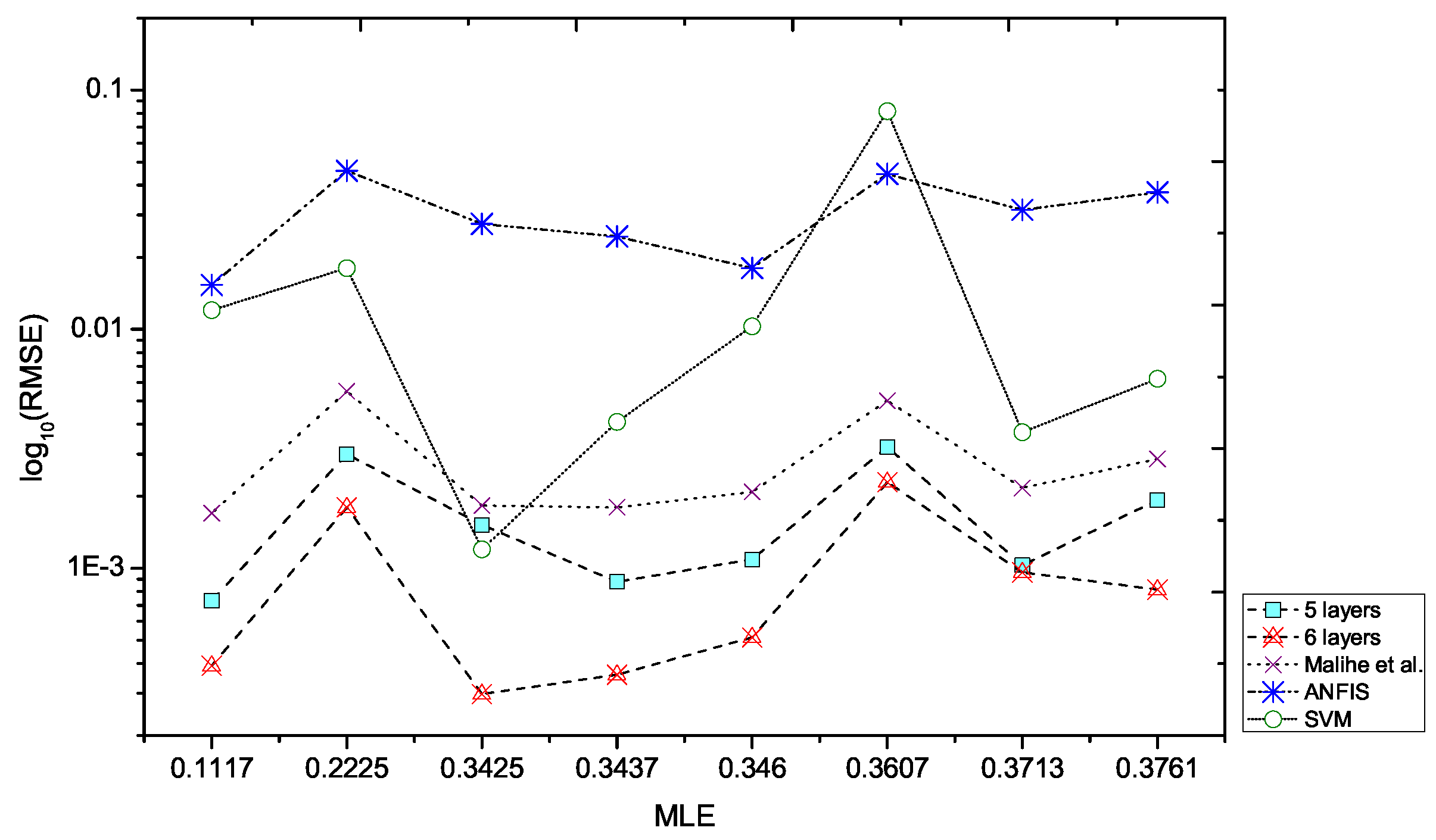
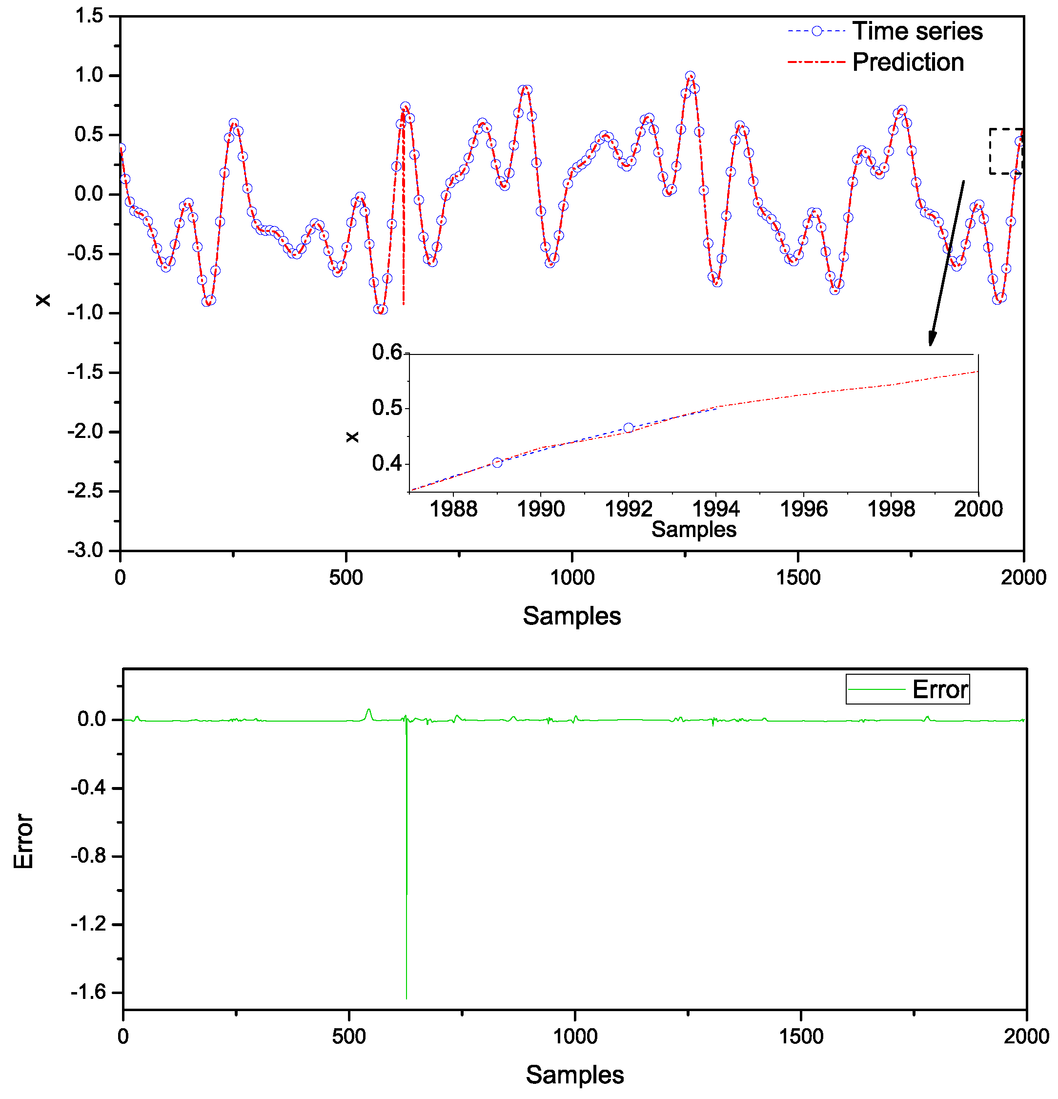
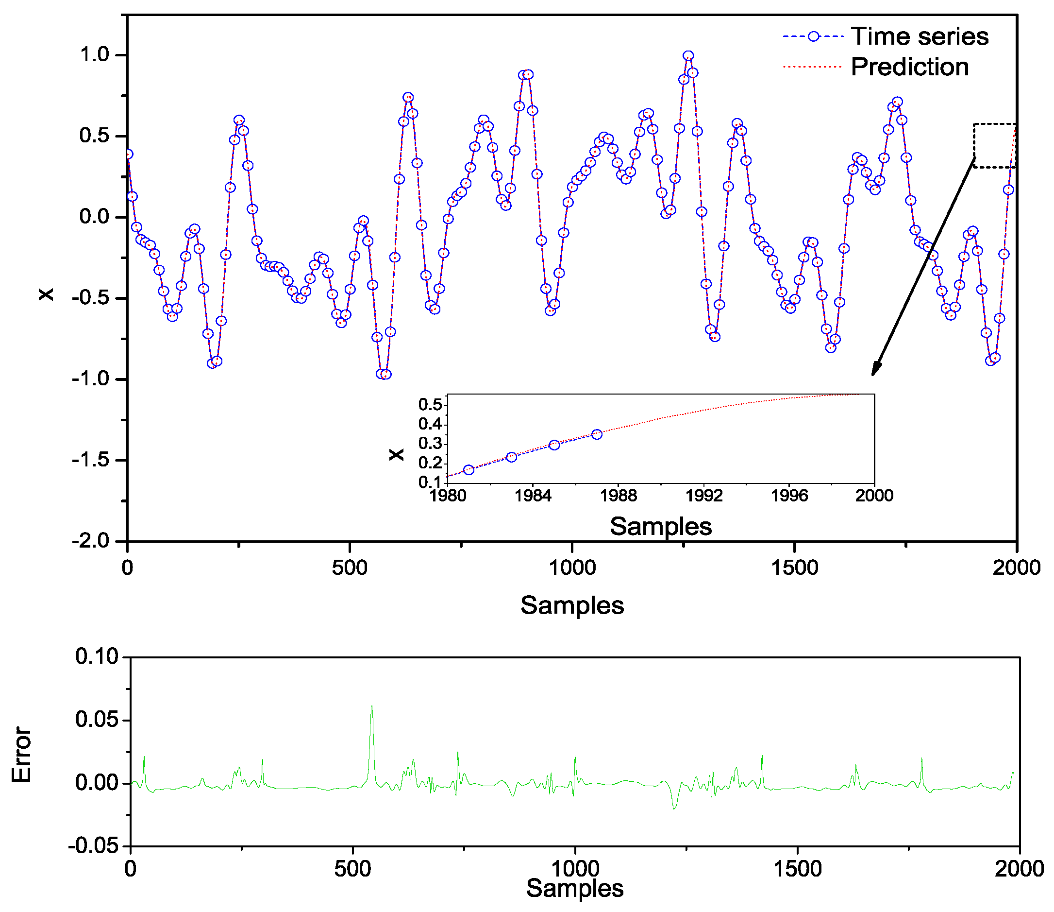
3.4. Chaotic Time Series Prediction by ANN, ANFIS and SVM
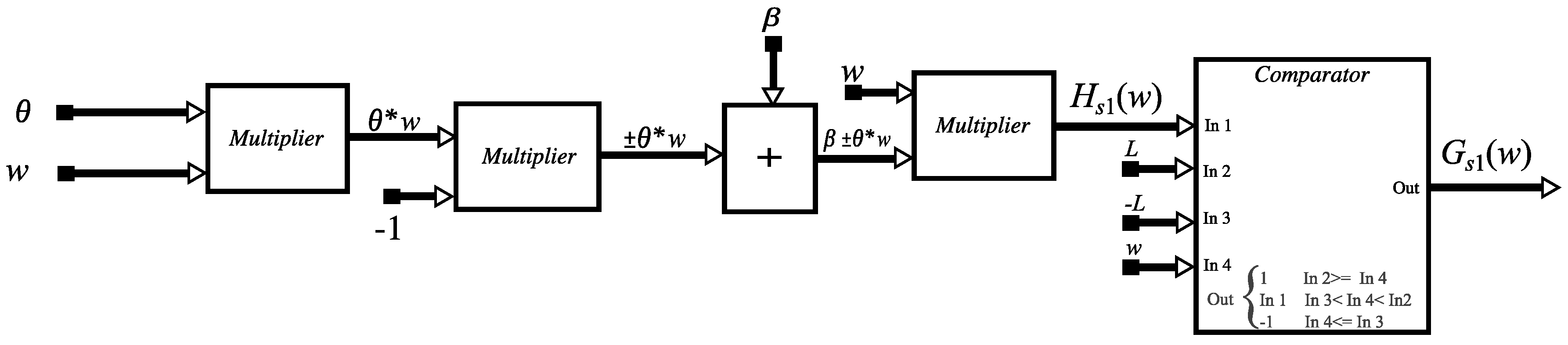
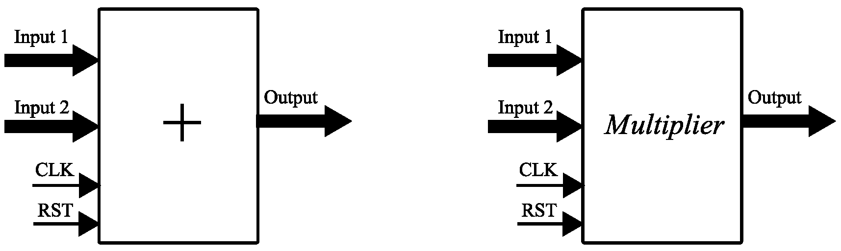
4. FPGA Implementation of an MLP
5. Conclusions
Author Contributions
Funding
Conflicts of Interest
References
- Pano-Azucena, A.D.; Tlelo-Cuautle, E.; Tan, S.X.D. Prediction of chaotic time series by using ANNs, ANFIS and SVMs. In Proceedings of the 7th International Conference on Modern Circuits and Systems Technologies (MOCAST), Thessaloniki, Greece, 7–9 May 2018; pp. 1–4. [Google Scholar]
- Stamatis, N.; Parthimos, D.; Griffith, T.M. Forecasting chaotic cardiovascular time series with an adaptive slope multilayer perceptron neural network. IEEE Trans. Biomed. Eng. 1999, 46, 1441–1453. [Google Scholar] [CrossRef] [PubMed]
- Ishikawa, M.; Moriyama, T. Prediction of time series by a structural learning of neural networks. Fuzzy Sets Syst. 1996, 82. [Google Scholar] [CrossRef]
- Aras, S.; Kocakoç, İ.D. A new model selection strategy in time series forecasting with artificial neural networks: IHTS. Neurocomputing 2016, 174, 974–987. [Google Scholar] [CrossRef]
- Pouzols, F.M.; Lendasse, A.; Barros, A.B. Autoregressive time series prediction by means of fuzzy inference systems using nonparametric residual variance estimation. Fuzzy Sets Syst. 2010, 161, 471–497. [Google Scholar] [CrossRef] [Green Version]
- Di Martino, F.; Loia, V.; Sessa, S. Fuzzy transforms method in prediction data analysis. Fuzzy Sets Syst. 2011, 180, 146–163. [Google Scholar] [CrossRef]
- Singh, P.; Borah, B. High-order fuzzy-neuro expert system for time series forecasting. Knowledge-Based Syst. 2013, 46, 12–21. [Google Scholar] [CrossRef]
- Thissen, U.; Van Brakel, R.; De Weijer, A.; Melssen, W.; Buydens, L. Using support vector machines for time series prediction. Chemom. Intell. Lab. Syst. 2003, 69, 35–49. [Google Scholar] [CrossRef]
- Kim, K.j. Financial time series forecasting using support vector machines. Neurocomputing 2003, 55, 307–319. [Google Scholar] [CrossRef]
- Ardalani-Farsa, M.; Zolfaghari, S. Chaotic time series prediction with residual analysis method using hybrid Elman–NARX neural networks. Neurocomputing 2010, 73, 2540–2553. [Google Scholar] [CrossRef]
- Bodyanskiy, Y.; Vynokurova, O. Hybrid adaptive wavelet-neuro-fuzzy system for chaotic time series identification. Inf. Sci. 2013, 220, 170–179. [Google Scholar] [CrossRef]
- Bagheri, A.; Peyhani, H.M.; Akbari, M. Financial forecasting using ANFIS networks with quantum-behaved particle swarm optimization. Expert Syst. Appl. 2014, 41, 6235–6250. [Google Scholar] [CrossRef]
- Delafrouz, H.; Ghaheri, A.; Ghorbani, M.A. A novel hybrid neural network based on phase space reconstruction technique for daily river flow prediction. Soft Comput. 2018, 22, 2205–2215. [Google Scholar] [CrossRef]
- Ravi, V.; Pradeepkumar, D.; Deb, K. Financial time series prediction using hybrids of chaos theory, multi-layer perceptron and multi-objective evolutionary algorithms. Swarm Evol. Comput. 2017, 36, 136–149. [Google Scholar] [CrossRef]
- Deo, R.C.; Wen, X.; Qi, F. A wavelet-coupled support vector machine model for forecasting global incident solar radiation using limited meteorological dataset. Appl. Energy 2016, 168, 568–593. [Google Scholar] [CrossRef]
- Kisi, O.; Parmar, K.S. Application of least square support vector machine and multivariate adaptive regression spline models in long term prediction of river water pollution. J. Hydrol. 2016, 534, 104–112. [Google Scholar] [CrossRef]
- Al-Mahasneh, M.; Aljarrah, M.; Rababah, T.; Alu’datt, M. Application of Hybrid Neural Fuzzy System (ANFIS) in Food Processing and Technology. Food Eng. Rev. 2016, 8, 351–366. [Google Scholar] [CrossRef]
- Melin, P.; Soto, J.; Castillo, O.; Soria, J. A new approach for time series prediction using ensembles of ANFIS models. Expert Syst. Appl. 2012, 39, 3494–3506. [Google Scholar] [CrossRef]
- Pano-Azucena, A.D.; Tlelo-Cuautle, E.; Tan, S. Electronic System for Chaotic Time Series Prediction Associated to Human Disease. In Proceedings of the 2018 IEEE International Conference on Healthcare Informatics (ICHI), New York, NY, USA, 4–7 June 2018; pp. 323–327. [Google Scholar]
- Tlelo-Cuautle, E.; de la Fraga, L.; Rangel-Magdaleno, J. Engineering Applications of FPGAs; Springer: New York, NY, USA, 2016. [Google Scholar]
- De la Fraga, L.G.; Tlelo-Cuautle, E.; Carbajal-Gómez, V.; Munoz-Pacheco, J. On maximizing positive Lyapunov exponents in a chaotic oscillator with heuristics. Rev. Mex. Fis. 2012, 58, 274–281. [Google Scholar]
- Carbajal-Gómez, V.H.; Tlelo-Cuautle, E.; Fernández, F.V. Optimizing the positive Lyapunov exponent in multi-scroll chaotic oscillators with differential evolution algorithm. Appl. Math. Comput. 2013, 219, 8163–8168. [Google Scholar] [CrossRef]
- Carbajal-Gómez, V.H.; Tlelo-Cuautle, E.; Fernández, F.V. Application of computational intelligence techniques to maximize unpredictability in multiscroll chaotic oscillators. In Computational Intelligence in Analog and Mixed-Signal (AMS) and Radio-Frequency (RF) Circuit Design; Springer: New York, NY, USA, 2015; pp. 59–81. [Google Scholar]
- Shiblee, M.; Kalra, P.K.; Chandra, B. Time Series Prediction with Multilayer Perceptron (MLP): A New Generalized Error Based Approach. In Advances in Neuro-Information Processing; Köppen, M., Kasabov, N., Coghill, G., Eds.; Springer: Berlin/Heidelberg, Germany, 2009; pp. 37–44. [Google Scholar]
- Masters, T. Practical Neural Network Recipes in C++; Morgan Kaufmann: Massachusetts, MA, USA, 1993. [Google Scholar]
- Molaie, M.; Falahian, R.; Gharibzadeh, S.; Jafari, S.; Sprott, J.C. Artificial neural networks: powerful tools for modeling chaotic behavior in the nervous system. Front. Comput. Neurosci. 2014, 8, 40. [Google Scholar] [CrossRef] [PubMed]
- Ye, Y.M.; Wang, X.D. Chaotic time series prediction using least squares support vector machines. Chin. Phys. 2004, 13, 454. [Google Scholar]
- Sapankevych, N.I.; Sankar, R. Time Series Prediction Using Support Vector Machines: A Survey. IEEE Comput. Intell. Mag. 2009, 4, 24–38. [Google Scholar] [CrossRef]
- Kwan, H. Simple sigmoid-like activation function suitable for digital hardware implementation. Electron. Lett. 1992, 28, 1379–1380. [Google Scholar] [CrossRef]


| Case | a | b | c | MLE | |
|---|---|---|---|---|---|
| 1 | 1.0000 | 1.0000 | 0.4997 | 1.0000 | 0.3761 |
| 2 | 1.0000 | 0.7884 | 0.6435 | 0.6665 | 0.3713 |
| 3 | 0.8661 | 1.0000 | 0.3934 | 0.9903 | 0.3607 |
| 4 | 0.7746 | 0.6588 | 0.5846 | 0.4931 | 0.3460 |
| 5 | 1.0000 | 0.7000 | 0.6780 | 0.1069 | 0.3437 |
| 6 | 1.0000 | 0.7000 | 0.7000 | 0.2542 | 0.3425 |
| 7 | 0.5610 | 0.9470 | 0.3460 | 0.6810 | 0.2225 |
| 8 | 0.7000 | 0.7000 | 0.7000 | 0.7000 | 0.1117 |
| Hidden Layers | Geometric Pyramid Rule | |
|---|---|---|
| 1 | ||
| 2 | ||
| 3 | ||
| ⋮ | ⋮ | ⋮ |
| i | ||
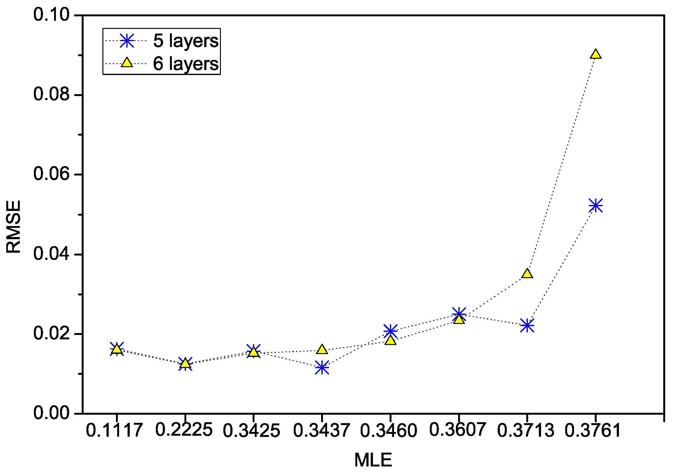
| Characteristics | MLP from [26] | MLP Applying the Geometric Pyramid Rule | |
|---|---|---|---|
| Number of layers | 6 | 5 | 6 |
| Number of neurons | |||
| Activation function | |||
| Learning algorithm | Levenberg–Marquardt algorithm | ||
| MLE | ANN | ANFIS | LS-SVM | ||
|---|---|---|---|---|---|
| 5 Layers | 6 Layers | [26] | |||
| 0.1117 | 7.31 × 10 | 3.91 × 10 | 1.70 × 10 | 0.0153 | 0.0120 |
| 0.2225 | 3.00 × 10 | 1.80 × 10 | 5.49 × 10 | 0.0460 | 0.0180 |
| 0.3425 | 1.52 × 10 | 2.98 × 10 | 1.83 × 10 | 0.0276 | 0.0012 |
| 0.3437 | 8.78 × 10 | 3.59 × 10 | 1.80 × 10 | 0.0244 | 0.0041 |
| 0.3460 | 1.09 × 10 | 5.14 × 10 | 2.09 × 10 | 0.0180 | 0.0103 |
| 0.3607 | 3.22 × 10 | 2.29 × 10 | 5.03 × 10 | 0.0446 | 0.0816 |
| 0.3713 | 1.03 × 10 | 9.63 × 10 | 2.17 × 10 | 0.0315 | 0.0037 |
| 0.3761 | 1.93 × 10 | 8.14 × 10 | 2.87 × 10 | 0.0373 | 0.0062 |
© 2018 by the authors. Licensee MDPI, Basel, Switzerland. This article is an open access article distributed under the terms and conditions of the Creative Commons Attribution (CC BY) license (http://creativecommons.org/licenses/by/4.0/).
Share and Cite
Pano-Azucena, A.D.; Tlelo-Cuautle, E.; Tan, S.X.-D.; Ovilla-Martinez, B.; De la Fraga, L.G. FPGA-Based Implementation of a Multilayer Perceptron Suitable for Chaotic Time Series Prediction. Technologies 2018, 6, 90. https://0-doi-org.brum.beds.ac.uk/10.3390/technologies6040090
Pano-Azucena AD, Tlelo-Cuautle E, Tan SX-D, Ovilla-Martinez B, De la Fraga LG. FPGA-Based Implementation of a Multilayer Perceptron Suitable for Chaotic Time Series Prediction. Technologies. 2018; 6(4):90. https://0-doi-org.brum.beds.ac.uk/10.3390/technologies6040090
Chicago/Turabian StylePano-Azucena, Ana Dalia, Esteban Tlelo-Cuautle, Sheldon X. -D. Tan, Brisbane Ovilla-Martinez, and Luis Gerardo De la Fraga. 2018. "FPGA-Based Implementation of a Multilayer Perceptron Suitable for Chaotic Time Series Prediction" Technologies 6, no. 4: 90. https://0-doi-org.brum.beds.ac.uk/10.3390/technologies6040090