A Space-Time Correlation Model for MRC Receivers in Rayleigh Fading Channels

Abstract

This paper presents a statistical model for maximum ratio combining (MRC) receivers in Rayleigh fading channels enabled with a temporal combining process. This means that the receiver effectively combines spatial and temporal branch components. Therefore, the signals that will be processed by the MRC receiver are collected not only across different antennas (space), but also at different instants of time. This suggests the use of a retransmission, repetition or space-time coding algorithm that forces the receiver to store signals in memory at different instants of time. Eventually, these stored signals are combined after a predefined or dynamically optimized number of time-slots or retransmissions. The model includes temporal correlation features in addition to the space correlation between the signals of the different components or branches of the MRC receiver. The derivation uses a frequency domain approach (using the characteristic function of the random variables) to obtain closed-form expressions of the statistics of the post-processing signal-to-noise ratio (SNR) under the assumption of equivalent correlation in time and equivalent correlation in space. The described methodology paves the way for the reformulation of other statistical functions as a frequency-domain polynomial root analysis problem. This is opposed to the infinite series approach that is used in the conventional methodology using directly the probability density function (PDF). The results suggest that temporal diversity is a good complement to receivers with limited spatial diversity capabilities. It is also shown that this additional operation could be maximized when the temporal diversity is adaptive (i.e., activated by thresholds of SNR), thus leading to a better resource utilization.

1. Introduction

Wireless technologies are becoming more pervasive, adaptive and reliable than ever before. They are at the core of the revolution of the Internet-of-Things (IoT) and 5G. This is mainly due to their flexible infrastructure, as well as a modern and adaptive radio technology with over-the-air troubleshooting, commissioning and maintenance capabilities [1,2,3].

The success of wireless solutions and the increased trust on IoT technology has created a growing demand for more reliable and faster (real-time) services. The new era of the IoT and machine-to-machine (M2M) communications dawns on emerging ultra-reliable, real-time and ultra-low-latency services (as part of 5G or beyond 5G). In order to achieve these objectives, highly dense multiple antenna technology also known as massive MIMO (multiple-input multiple-output) is being developed [4]. However, higher antenna densities usually lead to higher channel correlation figures [5]. In addition, since low latency design will be enforced, packet retransmissions (if any) will take place at higher frequencies (within less than 3 ms considering 1 ms frames), which also means they will experience higher temporal correlation.

This paper proposes a model for maximum-ratio combining (MRC) multiple antenna receivers that considers not only the diversity combining of all the copies of the signal received across the different antennas. The receiver also considers the repeated copies in the time domain due to a retransmission diversity or a space-time/repetition coding algorithm. This space-time model for MRC receivers assumes equivalent correlation in space and equivalent correlation in the time domain. This simplifies theoretical closed-form calculation, and it also allows us to include enriched physical layer information that is relevant for technologies with dense spatial and temporal processing requirements (e.g., ultra-low latency design with massive MIMO). We assume that, even in scenarios with high spatial diversity gains, ultra-low latency streams will experience residual errors due to a number of issues such as: non-orthogonal waveform interference, grant free uncoordinated (random) access collisions, deep fades or object shadowing, and high node density (inter-user interference). The residual errors mean that retransmissions and/or space-time coding are still necessary to transmit information correctly. All the spatial and temporal copies of the information will be combined to improve signal quality. The temporal copies will be received at higher frequencies than in previous technologies due to ultra short frame duration (1 ms or less), which means that higher temporal correlation values need to be considered. Our solution aims to help with considering these new challenging requirements in a theoretical tractable framework for space-time correlated MRC receivers. The model aims to be used in large scale simulations of wireless networks where the abstraction of the lower layers needs to be as compressed as possible to reduce complexity, but it also needs to provide a fair representation of the underlying PHY-layer.

This paper is organized as follows. Section 2 describes previous works and the achievements of this paper with respect to the state of the art. Section 3 describes the system model and the assumptions of the paper. Section 4 details the derivation of the performance model using a frequency domain interpretation. Section 5 presents analytic results and sketches of the statistics of signal-to-noise ratio (SNR). Finally, Section 6 presents the conclusions of the paper.

Notation: Bold lower case variables denote column vectors, e.g., $\mathbf{a}$. ${(·)}^T$ denotes the vector transpose operator, ${(·)}^{*}$ is the complex conjugate operator, and ${(·)}^H$ denotes the Hermitian vector transpose operator. $\mathcal{CN}(\mu ,{\sigma }^2)$ denotes the complex circular Gaussian distribution with mean $\mu$ and variance ${\sigma }^2$, $\mathcal{CN}({\mathbf{m}}_Q,{\sigma }^2{\mathbf{I}}_Q)$ denotes the multidimensional complex circular Gaussian distribution with mean vector ${\mathbf{m}}_Q$ (with length Q) and co-variance matrix ${\sigma }^2{\mathbf{I}}_Q$, where ${\mathbf{I}}_Q$ is the identity matrix of order Q. $E[·]$ is the statistical average operator. $f_X\left(x\right)$, ${\overline{F}}_X\left(x\right)$, and $F_X\left(x\right)$, denote, respectively, the probability density (PDF), complementary cumulative (CCDF), and cumulative density functions (CDF) of random variable X. $f_{X|Y}\left(x\right|y)$, ${\overline{F}}_{X|Y}\left(x\right|y)$, and $F_{X|Y}\left(x\right|y)$, denote, respectively, the PDF, CCDF, and CDF of r.v. X conditioned on an instance of r.v. Y. ${\mathrm{\Psi }}_X\left(s\right)$ and ${\mathrm{\Psi }}_{X|Y}\left(s\right)$ denote, respectively, the characteristic unction (CF) of the r.v. X and the CF of the r.v. X conditioned on an instance of the r.v. Y. Finally, $s=i\omega$ is the complex frequency variable.

2. Background and Previous Works

Multiple antenna systems have been extensively studied over the last few years. This is because they represent the main candidate to enable ultra-fast, reliable and real-time wireless critical networks (e.g., 5G) [6]. The simplest multiple antenna system is the MRC transceiver, which provides a relatively flexible framework for statistical analysis and abstraction modelling.

2.1. MRC Receiver Formulation

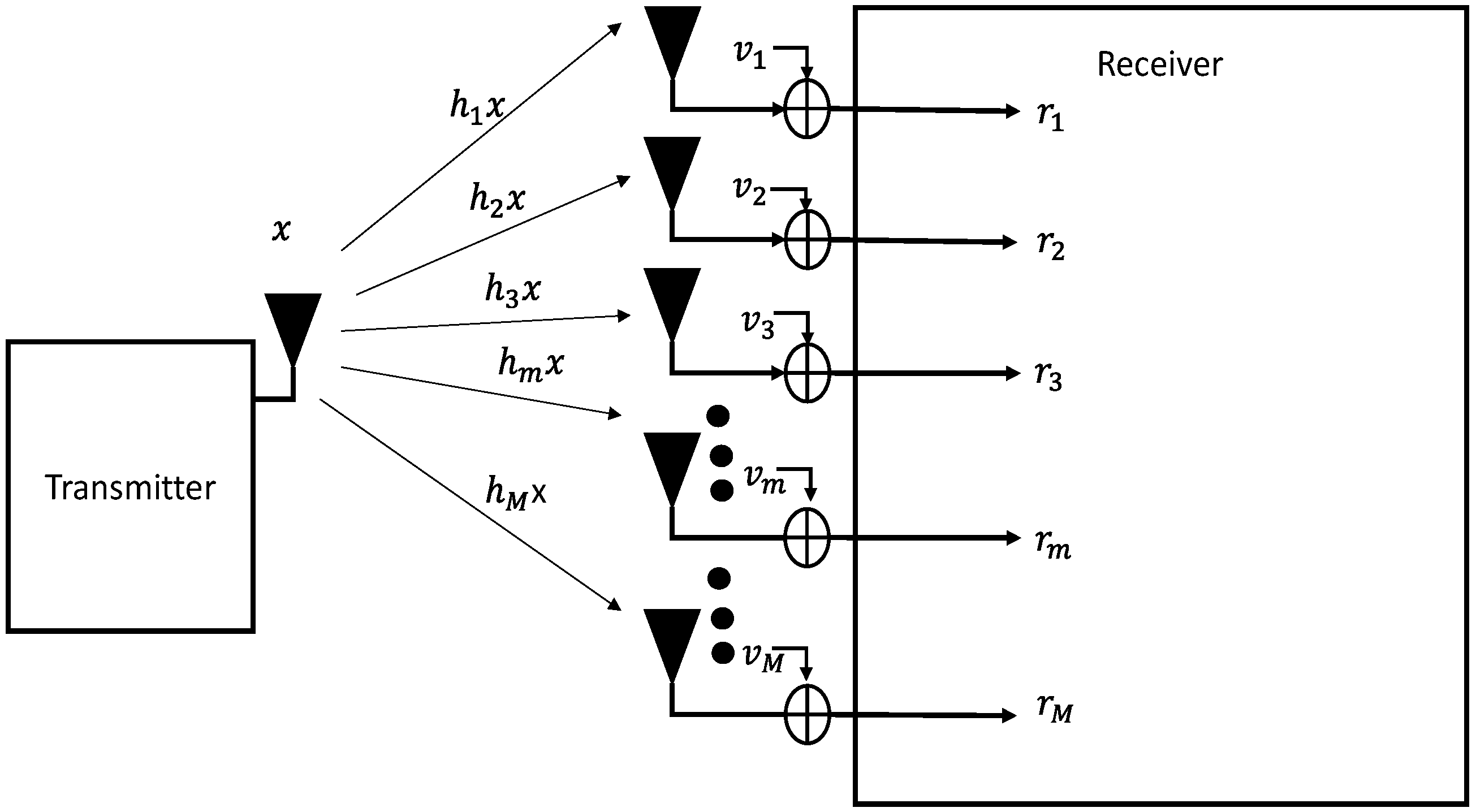
Consider the generic multiple antenna receiver in Figure 1 with M antennas. The channel between the transmitter and the mth antenna of the receiver is denoted by $h_m$. Consider that the transmitted symbol, denoted by x, has a unitary transmit power constraint $E\left[x^{*}x\right]=1$. The received signal $r_m$ in the mth branch or antenna can be expressed as:

$$r_m=h_{m}x+v_m,$$

(1)

where $v_m$ is the additive zero-mean white complex circular Gaussian noise with variance ${\sigma }_v^2$: $v_m\sim \mathcal{CN}(0,{\sigma }_v^2)$. The expression in (1) can be written in vector notation as follows:

$$\mathbf{r}=\mathbf{h}x+\mathbf{v},$$

(2)

where $\mathbf{r}={[r_1,r_2,...,r_m,...r_M]}^T$, $\mathbf{h}={[h_1,h_2,...,h_m,...,h_M]}^T$, and $\mathbf{v}={[v_1,v_2,...v_m,...,,v_M]}^T$. $\mathbf{v}$ is a vector of zero-mean Gaussian distributed noise with covariance matrix ${\sigma }_v^2{\mathbf{I}}_M$: $\mathbf{v}\sim \mathcal{CN}({\mathbf{0}}_M,{\sigma }_v^2{\mathbf{I}}_M)$.

The receiver processes the signals using the beam-forming Rx column vector $\mathbf{y}$. The post-processed signal ($\widehat{\mathbf{r}}$) and the post processing average signal-to-noise ratio (SNR), denoted by $\mathrm{\Gamma }$, can be thus expressed, respectively, as follows:

$$\widehat{\mathbf{r}}={\mathbf{y}}^H\mathbf{r}={\mathbf{y}}^H(\mathbf{h}x+\mathbf{v}),$$

(3)

and

$$\mathrm{\Gamma }=\frac{E\left[{\left({\mathbf{y}}^H\mathbf{h}\right)}^2\right]}{E\left[{\left({\mathbf{y}}^H\mathbf{v}\right)}^2\right]}.$$

(4)

The MRC receiver aims to maximize the SNR of a set of branches or sources of diversity when the channels or branches are statistically independent. This is achieved by using as beamforming processing vector the same channel vector:

$$\mathbf{y}=\mathbf{h}.$$

(5)

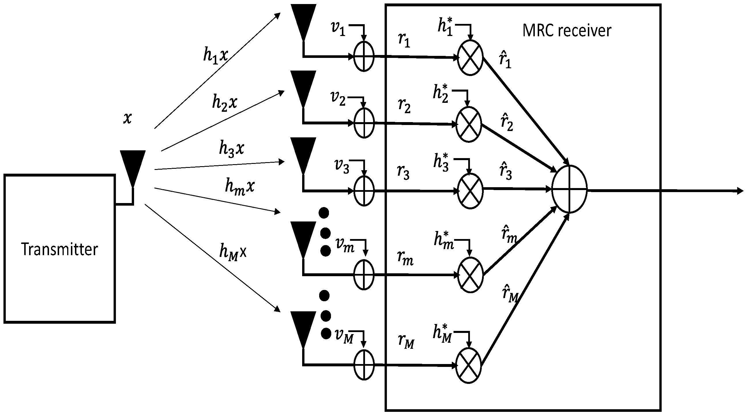
This selection can be shown to maximize the SNR in (4) when $E\left[\mathbf{h}{\mathbf{h}}^H\right]$ is a diagonal matrix, which means channels are spatially uncorrelated. The conventional MRC receiver is illustrated in Figure 2. This is opposed to other techniques such as equal gain combining (EGC), where the output of branches is simply averaged. EGC can be shown to be optimum in scenarios with high spatial correlation or with a predominant deterministic component. The EGC receiver is shown in Figure 3.

2.2. Previous Works

The literature of MRC transceivers has focused on the derivation of outage and bit error probability distributions (see [7,8,9,10,11,12,13,14,15,16,17]). The effects of imperfect channel knowledge at the receiver side of MRC systems in Rayleigh fading correlated channels can be found in [7,8]. Imperfect channel state information at the transmitter side with SINR-based resource allocation for correlated MRC receivers in Rayleigh fading channels was presented in our previous work in [9]. The bi-variate distribution of correlated Rayleigh distributions has been presented in [10]. The case of perfect channel estimation MRC distribution was presented in [11]. A series expansion of the statistics of MRC systems with correlated Rician channels is given in [12]. A unified approach for analysis of two-stage MRC systems with hybrid selection in generalized Rice correlated channels was proposed in [13]. Extensions to the case of co-channel interference are given in [14,15,16,17]. A recent review of works on MRC receivers with correlation has been presented in [18].

Joint terminal scheduling and beam-forming for MRC receivers with Rice correlated channels was presented in [19]. The authors in [20] have presented the multivariate distribution for Rice and Rayleigh fading channels with generalized correlation using additions of Gaussian random variables. In [21], the authors provided generalized Rayleigh, Rice and Nakagami distributions for Gaussian correlated random variables. The work in [22,23] suggests that channel correlation is not always an undesirable property. In low SNR scenarios, channel correlation seems to perform better than expected. This is because lack of diversity might be compensated with equal gain combining rather than the MRC combining philosophy.

The expressions for MRC and EGC receivers are well known in the case of uncorrelated or fully correlated channels. However, the topic of correlation is more complex and subject to a diverse set of assumptions. The first difficulty in analyzing correlated multiple antenna systems is to introduce correlation between the signals of the different branches or antennas. The correlation coefficients can be defined between the component Gaussian random variables, their circular complex variables or even between their quadratic functions.

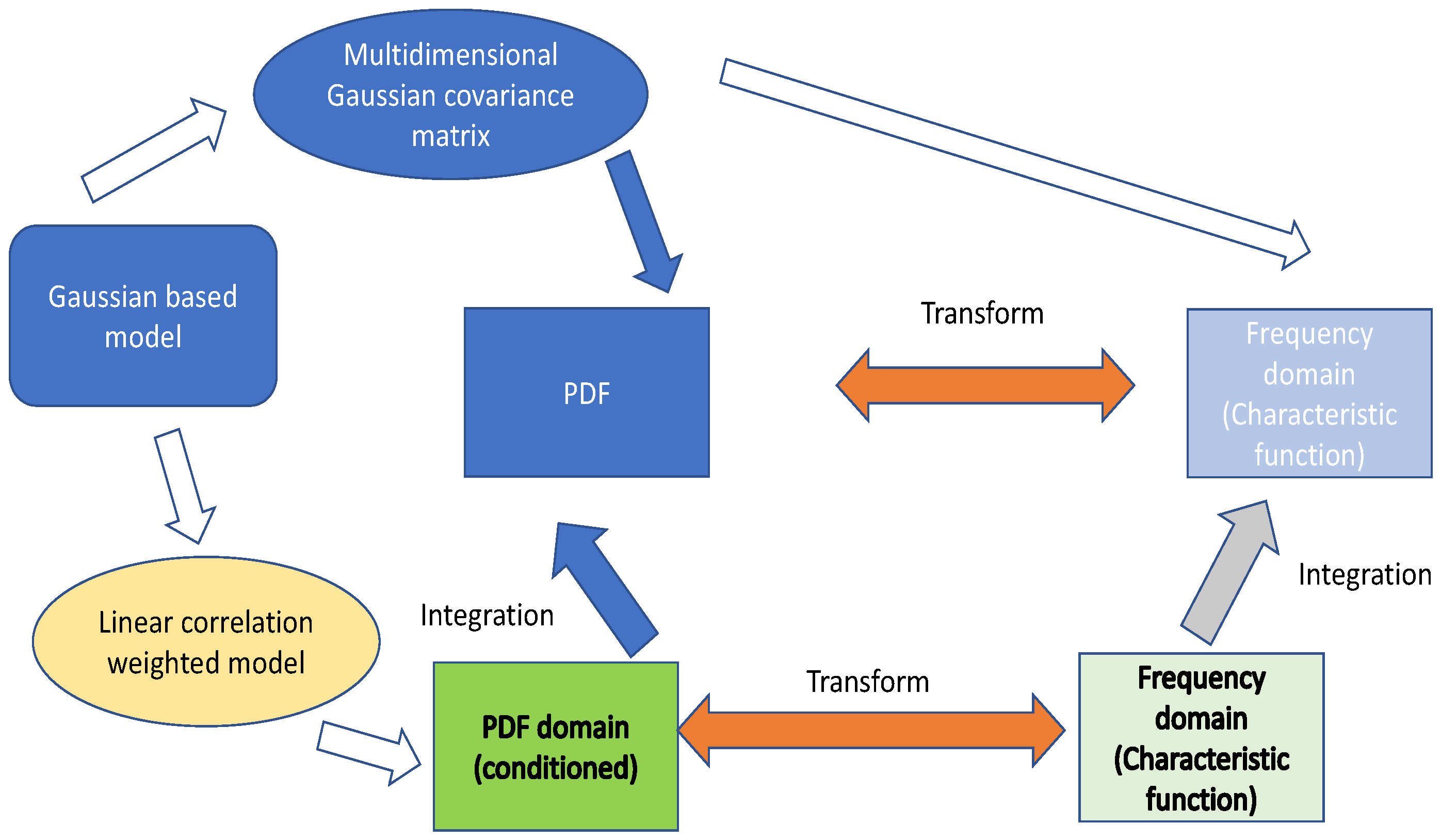
One method to introduce correlation in MRC receivers is to use the underlying multi-dimension Gaussian distribution and use different types of correlation matrix structure. This is usually exploited in multi-variate MRC distributions and for cases with exponential correlation (e.g., [24]). The final statistics are obtained by using transform operations over the base Gaussian correlated variables.

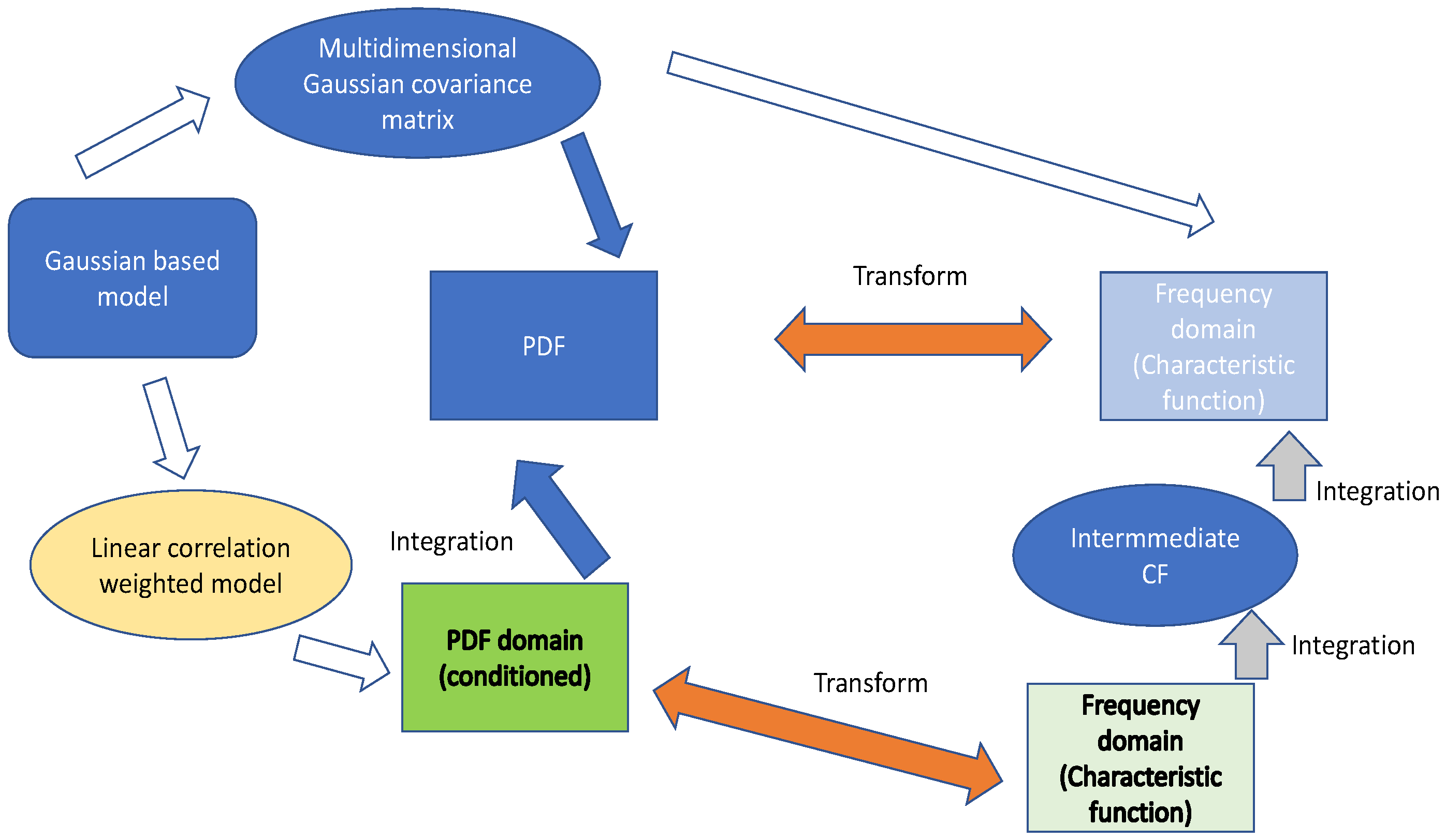
Another popular method to introduce correlation models in MRC receivers is to exploit the additive properties of Gaussian distributions. Linear correlation models introduce a weighted linear combination of independent Gaussian variables, where the weighting coefficients are directly related to the correlation coefficients. This method provides a quick way to introduce correlation properties in MRC receivers, and it also allows some simplified theoretical derivation. An overview of the different correlation models and the calculation of statistics in the PDF and in the frequency (characteristic function) domains is displayed in Figure 4. The work in [21] uses linear correlation models of the following type $G_m=\sqrt{1-{\lambda }^2}{Y}_m+{\lambda }_{m}Z$ to calculate the distribution of multivariate chi square distribution with correlation. Our previous work in [9] has used the following linear correlation model to calculate the performance of equi-correlated MRC receivers.

$$h_m=\sqrt{1-\rho }{Z}_m+\sqrt{\rho }G,$$

where $Z_m$ and G are auxiliary circular zero-mean independent Gaussian random variables and $\rho$ is the correlation coefficient. The work in [9] used a frequency domain approach to obtain the statistics of the SNR of the MRC receiver. The CCDF (complementary cumulative distribution function) of the post-processing SNR was found to be given by:

$${\overline{F}}_{\mathrm{\Gamma }}\left(y\right)=A{e}^{-\frac{y}{\overline{\gamma }}}+\sum _{m=2}^M\frac{B_m{y}^n}{{\tilde{\gamma }}^m(m-1)!}{e}^{-\frac{y}{\tilde{\gamma }}},$$

where $\tilde{\gamma }=(1-\rho )\gamma /{\sigma }_v^2$ and $\overline{\gamma }=M\rho \gamma /{\sigma }_v^2+\tilde{\gamma }$ and the coefficients are given by $A={(1-\tilde{\gamma }/\overline{\gamma })}^{1-M}$ and $B_m=(-\tilde{\gamma }/\overline{\gamma }){(1-\tilde{\gamma }/\overline{\gamma })}^{1-M}$. The present work aims to extend the work in [9] towards the use of an additional temporal combining strategy of signals collected in different instants of time or time-slots.

Summarizing, the contributions of this paper are the following:

• Extension of MRC receivers (conventionally analyzed in the space domain) to the time domain. This means the use of either a retransmission diversity mechanism or a space-time coding repetition approach.
• The MRC performance model uses spatial and temporal correlation coefficients. To the best of our knowledge, this is not commonly used in the literature of MRC receivers, and
• A frequency-domain approach (via the characteristic function) is used to calculate the statistics of the space-time MRC receiver. The result is a polynomial function whose roots can be obtained via numerical methods. The inverse transform is then used to obtain the exact probability density function (PDF). This is opposed to conventional methodologies where all conditioning and integration work are conducted exclusively in the PDF domain, which in some cases can lead to complex infinite series expressions.

3. System Model

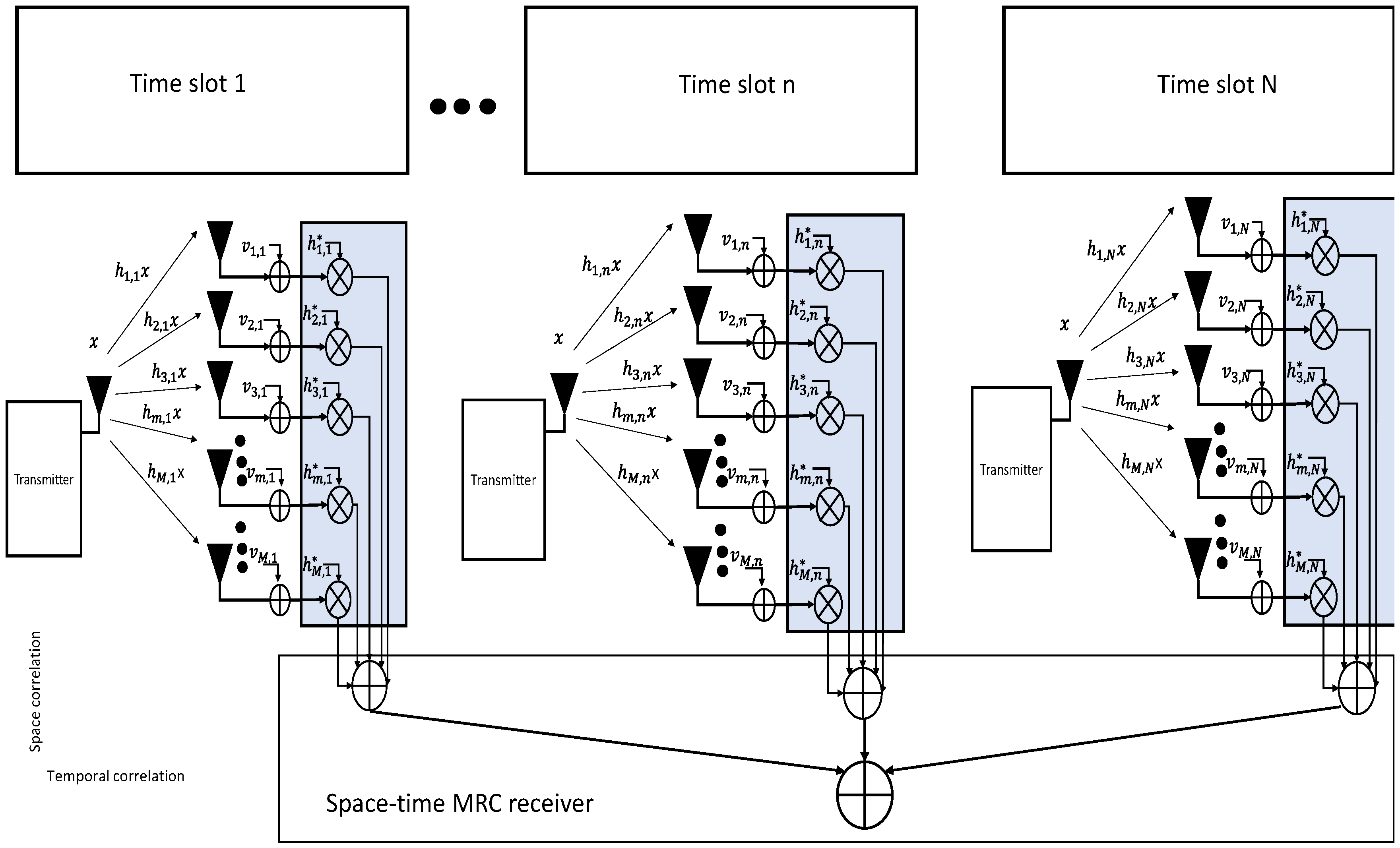
Consider the scenario depicted in Figure 5 with one antenna transmitter and an M antenna receiver using a retransmission or a space-time repetition coding algorithm that occupies N time slots. The channel between the transmitter and the mth antenna of the receiver in time slot n is denoted by $h_{m,n}$ and will be modeled as a zero-mean circular complex Gaussian random variable with variance $\gamma$: $h_{m,n}\sim \mathcal{CN}(0,\gamma )$. All channel variables will be modeled using a correlation model described in the following equation:

$$h_{m,n}=\sqrt{1-{\rho }_s^2-{\rho }_t^2}{Z}_{m,n}+{\rho }_s{Y}_n+{\rho }_t{W}_m,$$

(6)

where ${\rho }_s$ and ${\rho }_t$ are the spatial and temporal correlation coefficients, respectively, and $Z_{m,n}$, $Y_n$ and $W_m$ are independent and identically distributed circular Gaussian complex variables with variance $\gamma$: $\mathcal{CN}(0,\gamma )$. The previous model complies with the following expressions:

$$E\left[h_{m,n}^{*}{h}_{m,\tilde{n}}\right]={\rho }_t^2\gamma ,$$

and

$$E\left[h_{m,n}^{*}{h}_{\tilde{m},n}\right]={\rho }_s^2\gamma .$$

A list of the main variables in this paper is given in

Table 1. List of main variables.

Variable	Meaning
$h_{m,n}$	Channel between the terminal and antenna m in time slot n
M	Number of Rx antennas.
N	Number of time slots.
$\gamma$	Channel variance
${\rho }_s$	Space correlation coefficient
${\rho }_t$	Temporal correlation coefficient
$\mathbf{r}$	Rx Signal
$\mathbf{v}$	Noise vector at the receiver

. Consider the transmitted symbol x with unitary power constraint $E\left[x^{*}x\right]=1$. The signal received in antenna m at time slot n is given by:

$$r_{m,n}=h_{m,n}x+v_{m,n},$$

where $v_{m,n}$ is the complex circular Gaussian noise with zero mean and unit variance: $v_{m,n}\sim \mathcal{CN}(0,1)$. Stacking all the received signals in vector variables we obtain:

$$\mathbf{r}=\mathbf{h}x+\mathbf{v},$$

where $\mathbf{h}$ and $\mathbf{v}$ are the vectors of stacked channel and noise components, respectively. We can process the signals using a maximum ratio combining as follows:

$$\widehat{\mathbf{r}}={\mathbf{h}}^H\mathbf{r}.$$

The post processing signal to noise ratio (SNR) of the MRC receiver can be thus expressed as follows:

$${\mathrm{\Gamma }}_n=\sum _{k=1}^n\sum _{m=1}^M{\left|h_{m,k}\right|}^2.$$

(7)

4. Statistics Derivation

This section presents the derivation of statistics of the post processing SNR following a frequency domain approach. The methodology is illustrated in Figure 6, and explained briefly as follows. A characteristic function conditioned on the auxiliary random variables is proposed in the first place. The unconditioned characteristic function can be obtained by averaging (integration) over the PDF of the auxiliary variables. Then, the unconditioned PDF can be obtained by the inverse transform (Direct Fourier Transform). This method is opposite to the direct path of using the PDF conditioned on the auxiliary variables. This is followed by an averaging operation over the PDF of the auxiliary variables to obtain the desired expression. Commonly, this direct approach leads to complex infinite series expressions of the PDFs. While the frequency domain approach implies additional and complex averaging and transform operations, it can provide several advantages regarding interpretation of frequency components, or even simplified closed-form expressions. This paper proposes a frequency domain approach, but, instead of having one integration step, we do successive integration steps due to the complexity of the linear correlation model for space-time MRC receivers.

4.1. First Stage

Let us substitute the correlation model given by (6) in the expression of the post processing SNR given by (7), which yields:

$${\mathrm{\Gamma }}_n=\sum _{k=1}^n\sum _{m=1}^M{\left|\sqrt{1-{\rho }_s^2-{\rho }_t^2}{Z}_{m,k}+{\rho }_s{Y}_k+{\rho }_t{W}_m\right|}^2.$$

(8)

Consider the previous expression for the post-processing SNR conditioned on a fixed value of the r.v.s $Y_k$ and $W_m$. This can be identified as a non-central chi square distribution or the summation of the squares of complex Gaussian variables $\sqrt{1-{\rho }_s^2-{\rho }_t^2}{Z}_{m,k}$ with mean given by ${\rho }_s{Y}_k+{\rho }_t{W}_m$. The characteristic function (CF) of the r.v. ${\mathrm{\Gamma }}_n$ conditioned on the r.v.s $Y_k$ and $W_m$ is thus given by:

$${\mathrm{\Psi }}_{{\mathrm{\Gamma }}_n|{\tilde{Y}}_k,{\tilde{W}}_m}\left(s\right)=\frac{1}{{(1-s\tilde{\gamma })}^{Mn}}\prod _{m,k}{e}^{\frac{s|{\tilde{Y}}_k+{\tilde{W}}_m{|}^2}{1-s\tilde{\gamma }}}$$

(9)

where ${\tilde{Y}}_k={\rho }_s{Y}_k$, ${\tilde{W}}_m={\rho }_t{W}_m$, and $\tilde{\gamma }=(1-{\rho }_s^2-{\rho }_t^2)\gamma$. This can be rewritten as follows:

$${\mathrm{\Psi }}_{{\mathrm{\Gamma }}_n|{\tilde{Y}}_k,{\tilde{W}}_m}\left(s\right)=\frac{1}{{(1-s\tilde{\gamma })}^{Mn}}{e}^{{\sum }_{m,k}\frac{s|{\tilde{Y}}_k+{\tilde{W}}_m{|}^2}{1-s\tilde{\gamma }}}=\frac{1}{{(1-s\tilde{\gamma })}^{Mn}}{e}^u,$$

(10)

where

$$u=\sum _{k=1}^n\sum _{m=1}^M\alpha {\left|{\tilde{Y}}_k+{\tilde{W}}_m\right|}^2,$$

(11)

and

$$\alpha =\frac{s}{1-s\tilde{\gamma }}.$$

(12)

Let us now expand the quadratic function in (11) in terms of the $Y_k$ variables as follows:

$$u=\sum _{k=1}^n\left[{\left(\sqrt{M\alpha }{\tilde{Y}}_k+\frac{{\sum }_{m=1}^M\alpha {\tilde{W}}_m}{\sqrt{M\alpha }}\right)}^2\right.+\left.\sum _{m=1}^M\alpha {\left|{\tilde{W}}_m\right|}^2-{\left|\frac{{\sum }_{m=1}^M\alpha {\tilde{W}}_m}{\sqrt{M\alpha }}\right|}^2\right].$$

(13)

The expression of the r.v. u in (13) conditioned on the r.v.s ${\tilde{W}}_m$ can be identified as another non-central chi square distribution with n degrees of freedom. This leads to another integration/consitioning stage.

4.2. Second Stage

The CF of the r.v. u (13) conditioned on ${\tilde{W}}_m$ can be written as follows:

$${\mathrm{\Psi }}_{u|{\tilde{W}}_m}\left(\tilde{s}\right)=\frac{1}{{(1-\tilde{s}\overline{\gamma })}^n}{e}^{\frac{\tilde{s}n{\mu }_u}{1-\tilde{s}\overline{\gamma }}}{e}^{n\tilde{s}{\delta }_u},$$

(14)

where:

$${\mu }_u={\left|\frac{{\sum }_{m=1}^M\alpha {\tilde{W}}_m}{\sqrt{M\alpha }}\right|}^2,{\delta }_u=\sum _{m=1}^M\alpha |{\tilde{W}}_m{|}^2-{\left|\frac{{\sum }_{m=1}^M\alpha {\tilde{W}}_m}{\sqrt{M\alpha }}\right|}^2,\mathrm{and}\overline{\gamma }={\left|{\rho }_s\right|}^{2}M\alpha \gamma .$$

Let us rewrite the previous CF expression as follows:

$${\mathrm{\Psi }}_{u|y_1}\left(\tilde{s}\right)=\frac{1}{{(1-\tilde{s}\overline{\gamma })}^n}{e}^{y_1},$$

(15)

where

$$y_1={\left|\sqrt{{\lambda }_1}{\tilde{W}}_1+\frac{{\sum }_{m=2}^M{\eta }_1{\tilde{W}}_m}{\sqrt{{\lambda }_1}}\right|}^2+{\lambda }_1\sum _{m=2}^M{\left|{\tilde{W}}_m\right|}^2-{\left|\frac{{\sum }_{m=2}^M{\eta }_1{\tilde{W}}_m}{\sqrt{{\lambda }_1}}\right|}^2,$$

(16)

$${\lambda }_1=\frac{\tilde{s}n\alpha /M}{(1-\tilde{s}\overline{\gamma })}-n\tilde{s}\alpha (1-1/M)\mathrm{and}{\eta }_1=\frac{\tilde{s}n\alpha /M}{(1-\tilde{s}\overline{\gamma })}+n\tilde{s}\alpha /M.$$

The new r.v. $y_1$ in (16) is another square of Gaussian r.v.s. Conditioned on all the values of ${\tilde{W}}_m$ for $m>1$, the r.v. can be proved to have a shifted non-central chi square distribution of order 1. The analysis of this conditioning of the r.v. $y_1$ on the remiainign r.v.s leads to the third stage.

4.3. Third Stage

The CF of the r.v $y_1$ conditioned on the r.v. $y_2$ can be written as follows:

$${\mathrm{\Psi }}_{y_1|y_2}\left(s_1\right)=\frac{1}{1-s_1{\lambda }_1}{e}^{\frac{s_1{\mu }_1}{1-s_1{\lambda }_1}}{e}^{s_1{\delta }_1}=\frac{1}{1-s_1{\lambda }_1}{e}^{y_2},$$

(17)

where

$${\mu }_1={\left|\frac{{\sum }_{m=2}^M{\eta }_1{\tilde{W}}_m}{\sqrt{{\lambda }_1}}\right|}^2,\mathrm{and}{\delta }_1={\lambda }_1\sum _{m=2}^M{\left|{\tilde{W}}_m\right|}^2-{\left|\frac{{\sum }_{m=2}^M{\eta }_1{\tilde{W}}_m}{\sqrt{{\lambda }_1}}\right|}^2.$$

Let us write now the explicit expression for the r.v. $y_2$ as follows:

$$y_2={\left|\sqrt{{\lambda }_2}{\tilde{W}}_2+\frac{{\sum }_{m=3}^M{\eta }_2{\tilde{W}}_m}{\sqrt{{\lambda }_2}}\right|}^2+{\lambda }_2\sum _{m=3}^M{\left|{\tilde{W}}_m\right|}^2-{\left|\frac{{\sum }_{m=3}^M{\eta }_2{\tilde{W}}_m}{\sqrt{{\lambda }_2}}\right|}^2,$$

(18)

where

$${\lambda }_2=\frac{s_1{\eta }_1-s_1(1-s_1{\lambda }_1)({\lambda }_1^2-{\eta }_1^2)}{{\lambda }_1(1-s_1{\lambda }_1)},\mathrm{and}{\eta }_2=\frac{s_1{\eta }_1+s_1(1-s_1{\lambda }_1){\eta }_1^2}{{\lambda }_1(1-s_1{\lambda }_1)}.$$

The previous equations can be generalized to the $m-1$th component as follows:

$$y_{m-1}={\left|\sqrt{{\lambda }_{m-1}}{\tilde{W}}_{m-1}+\frac{{\sum }_{k=m}^M{\eta }_{m-1}{\tilde{W}}_k}{\sqrt{{\lambda }_{m-1}}}\right|}^2+{\lambda }_{m-1}\sum _{k=m}^M{\left|{\tilde{W}}_k\right|}^2-{\left|\frac{{\sum }_{k=m}^M{\eta }_{m-1}{\tilde{W}}_k}{\sqrt{{\lambda }_{m-1}}}\right|}^2,$$

(19)

$${\mathrm{\Psi }}_{y_{m-1}|y_m}\left(s_{m-1}\right)=\frac{1}{1-s_{m-1}{\lambda }_{m-1}}{e}^{\frac{s_{m-1}{\mu }_{m-1}}{1-s_{m-1}{\lambda }_{m-1}}}{e}^{s_{m-1}{\delta }_{m-1}}=\frac{1}{1-s_{m-1}{\lambda }_{m-1}}{e}^{y_m},$$

(20)

where

$${\mu }_{m-1}={\left|\frac{{\sum }_{k=m}^M{\eta }_k{\tilde{W}}_k}{\sqrt{{\lambda }_{m-1}}}\right|}^2,\mathrm{and}{\delta }_{m-1}={\lambda }_{m-1}\sum _{k=m}^M{\left|{\tilde{W}}_k\right|}^2-{\left|\frac{{\sum }_{k=m}^M{\eta }_{m-1}{\tilde{W}}_k}{\sqrt{{\lambda }_{m-1}}}\right|}^2.$$

Now, the expressions for the mth variable result in:

$$y_m={\left|\sqrt{{\lambda }_m}{\tilde{W}}_m+\frac{{\sum }_{k=m+1}^M{\eta }_m{\tilde{W}}_k}{\sqrt{{\lambda }_m}}\right|}^2+{\lambda }_m\sum _{k=m+1}^M{\left|{\tilde{W}}_k\right|}^2-{\left|\frac{{\sum }_{k=m+1}^M{\eta }_m{\tilde{W}}_k}{\sqrt{{\lambda }_m}}\right|}^2,$$

(21)

$${\lambda }_m=\frac{s_{m-1}{\eta }_{m-1}-s_{m-1}(1-s_{m-1}{\lambda }_{m-1})({\lambda }_{m-1}^2-{\eta }_1^2)}{{\lambda }_{m-1}(1-s_{m-1}{\lambda }_{m-1})},$$

and

$${\eta }_m=\frac{s_{m-1}{\eta }_{m-1}+s_{m-1}(1-s_{m-1}{\lambda }_{m-1}){\eta }_{m-1}^2}{{\lambda }_{m-1}(1-s_{m-1}{\lambda }_{m-1})}.$$

Let us now write the equations for the $M-1$th random variable:

$$y_{M-1}={\left|\sqrt{{\lambda }_{M-1}}{\tilde{W}}_{M-1}+\frac{{\eta }_{M-1}{\tilde{W}}_M}{\sqrt{{\lambda }_{M-1}}}\right|}^2+{\lambda }_m{\left|{\tilde{W}}_M\right|}^2-{\left|\frac{{\eta }_{M-1}{\tilde{W}}_M}{\sqrt{{\lambda }_{M-1}}}\right|}^2,$$

(22)

$${\mathrm{\Psi }}_{y_{M-1}|y_M}\left(s_{M-1}\right)=\frac{1}{1-s_{M-1}{\lambda }_{M-1}}{e}^{\frac{s_{M-1}{\mu }_{M-1}}{1-s_{M-1}{\lambda }_{M-1}}}{e}^{s_{M-1}{\delta }_{M-1}}=\frac{1}{1-s_{M-1}{\lambda }_{M-1}}{e}^{y_M}$$

(23)

where

$${\mu }_{M-1}={\left|\frac{{\eta }_{M-1}{\tilde{W}}_M}{\sqrt{{\lambda }_{M-1}}}\right|}^2,\mathrm{and}{\delta }_{M-1}={\lambda }_{M-1}{\left|{\tilde{W}}_M\right|}^2-{\left|\frac{{\eta }_{M-1}{\tilde{W}}_M}{\sqrt{{\lambda }_{M-1}}}\right|}^2.$$

We now write now the explicit expression for the r.v. $y_M$ as follows:

$$y_M={\left|\sqrt{{\lambda }_M}{\tilde{W}}_M\right|}^2,$$

(24)

where

$${\lambda }_M=\frac{s_{M-1}{\eta }_{M-1}-s_{M-1}(1-s_{M-1}{\lambda }_{M-1})({\lambda }_{M-1}^2-{\eta }_{M-1}^2)}{{\lambda }_{M-1}(1-s_{M-1}{\lambda }_{M-1})}.$$

The CF of the r.v. $y_M$ can be expressed as follows:

$${\mathrm{\Psi }}_{y_M}\left(s_M\right)=\frac{1}{1-s_M{\lambda }_M}.$$

(25)

4.4. Final Statistics

The CF of the SNR $\mathrm{\Gamma }$ can be obtained by the following formula:

$${\mathrm{\Psi }}_{\mathrm{\Gamma }}\left(s\right)=\frac{1}{{(1-s\tilde{\gamma })}^{Mn}}\frac{1}{{(1-\overline{\gamma })}^n}\prod _{m=1}^M\frac{1}{1-{\lambda }_m}.$$

(26)

See Appendix A for the proof. This equation can be solved using numerical tools resulting in a polynomial equation in terms of the frequency domain variable s. This CF can be regarded as the ratio of two polynomials in the frequency domain:

$${\mathrm{\Psi }}_{{\mathrm{\Gamma }}_n}\left(s\right)=\frac{H\left(s\right)}{G\left(s\right)}.$$

(27)

The roots of the denominator lead to the following partial fraction expansion:

$${\mathrm{\Psi }}_{{\mathrm{\Gamma }}_n}\left(s\right)=\sum _l\sum _{j=1}^{P\left(l\right)}\frac{A_{l,j}\left(s\right)}{{(1-{\gamma }_{l}s)}^j},$$

(28)

where $P\left(l\right)$ is the multiplicity of the lth root of the polynomial in the denominator, ${\gamma }_l$ is the lth root, and $A_{l,j}\left(s\right)={\sum }_{q=1}^{N(l,j)}{a}_q^{l,j}{s}^q$, $N(l,j)$ is the degree of the polynomial of the numerator of the lth root. This yields a back transform of the following form:

$${\overline{F}}_{{\mathrm{\Gamma }}_n}\left(y\right)=\sum _l\sum _{j=1}^{P\left(l\right)}\sum _{q=1}^{N(l,j)}\frac{d^q}{d}{a}_q^{l,j}{y}^j{e}^{-\frac{y}{{\gamma }_l}}.$$

(29)

This concludes the derivation of the statistics of SNR for the space time correlation model.

4.5. Adaptive Activation

In the time domain of the proposed MRC receiver model, the number of time slots used to create diversity can be known a priori (pre-allocated) or they can be adaptively selected. In the case explored in this subsection, the next retransmission of information only occurs if the SNR has surpassed the threshold $\beta$. In this adaptive scenario, we are interested in deriving the statistics of the SNR conditioned on the previous outcomes not achieving the desired threshold. It can be shown that (see Appendix B) the CDF of the SNR in time slot n conditioned on the SNR in time slot $n-1$ being below a given reception threshold can be expressed as follows:

$$F_{{\mathrm{\Gamma }}_n|{\mathrm{\Gamma }}_{n-1}<\beta }\left(\beta \right)=\frac{F_{{\mathrm{\Gamma }}_n}\left(\beta \right)}{F_{{\mathrm{\Gamma }}_{n-1}\left(\beta \right)}}.$$

(30)

This expression captures the effects of the combined branches in memory of the space-time receiver to have a truncated SNR excursion. This allows the system to utilize resources more efficiently, mainly because, if a certain level of SNR has been achieved with less time-slots than previously designed, channel utilization can be improved and another transmission can be scheduled in the vacant time-slots. The assumption of an SNR threshold for the evaluation of correct packet reception is used in many different settings of wireless networks. This facilitates analysis and introduces a performance metric for correct packet reception. In practice, however, correct packet reception depends on several other factors, such as error correction coding, modulation format, etc., so the use of a packet reception threshold based on SNR must be accompanied by a block error rate metric that depends on the transmission technology to be used.

5. Results

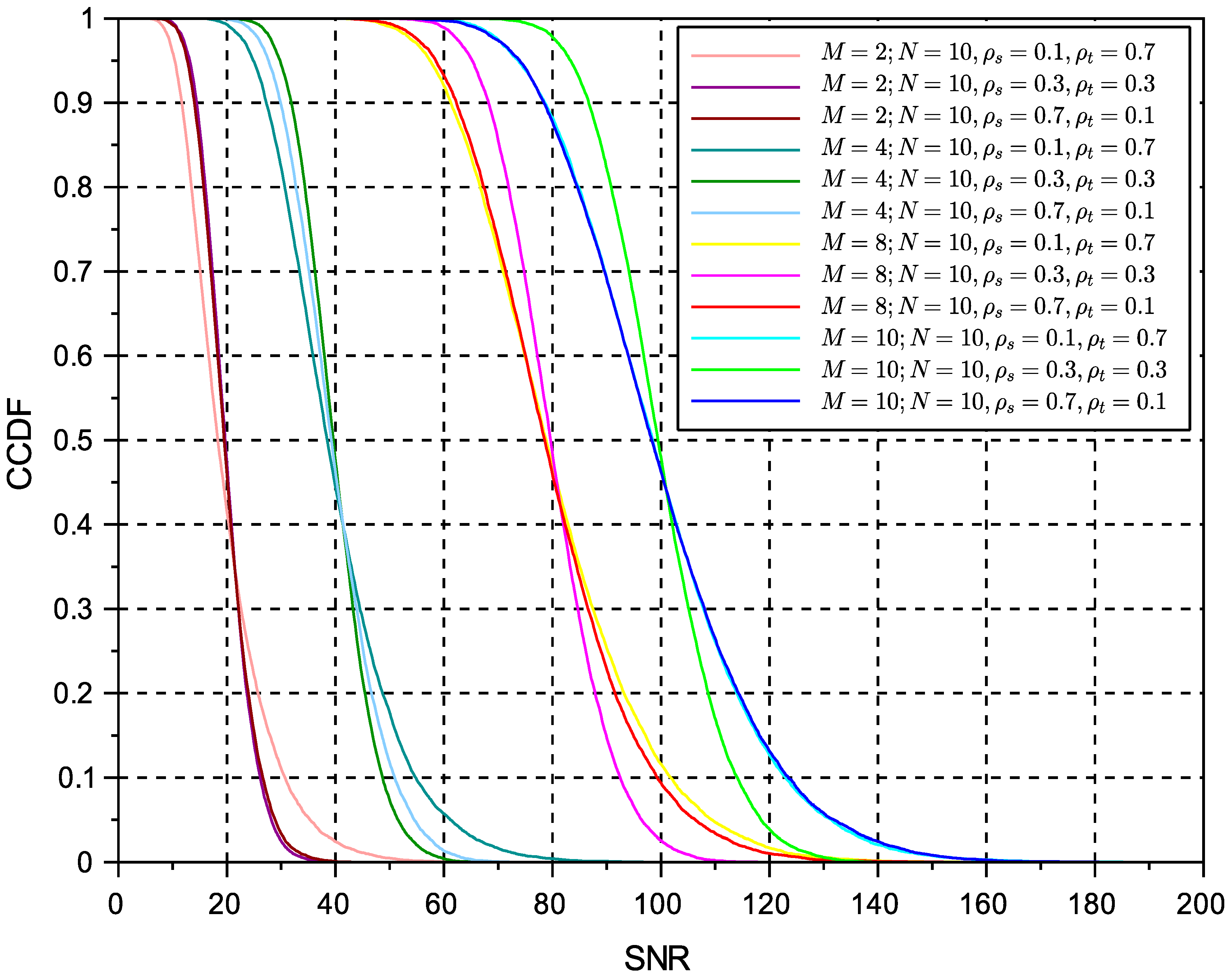
The results in this section have been obtained under a unitary transmit power value $\gamma =1$. Different numbers of antennas and time slots have been used to investigate the statistics of the SNR of the proposed space-time receiver. The target of our analysis is the complementary cumulative distribution function (CCDF) of the post processing SNR using the space time correlation model described in previous sections. Different values of correlation coefficient have also been used in space and time to verify the effects on performance. We select three values for each coefficient, using a maximum number of 10 time slots $N=10$ and different values of Rx antennas ($M=2,4,8,10$). A summary of the parameters used for evaluation is given in

Table 2. System evaluation parameters.

Variable	Value
M	Variable from 2 to 10
$\gamma$	1.
$\beta$	$Mn$.
${\rho }_s$	Variable: 0.1, 0.3, 0.7
${\rho }_t$	Variable: 0.1, 0.3, 0.7
N	set to 10 time slots

.

The results in Figure 7 show that the number of antennas or time slots shift to the right the CDF curves, which is an improvement on the post processing performance. In terms of the correlation coefficient, we observe a mixed behaviour. The CDF lines cross each other in general for the same number of antennas and time slots but with different values of space or time correlation. It seems that, at low SNR, higher correlation yields better performance, whereas, at high SNR, uncorrelated values have better behaviour. It seems that this differential effect between higher and lower correlation is amplified with the number of diversity sources, either in time or space domain.

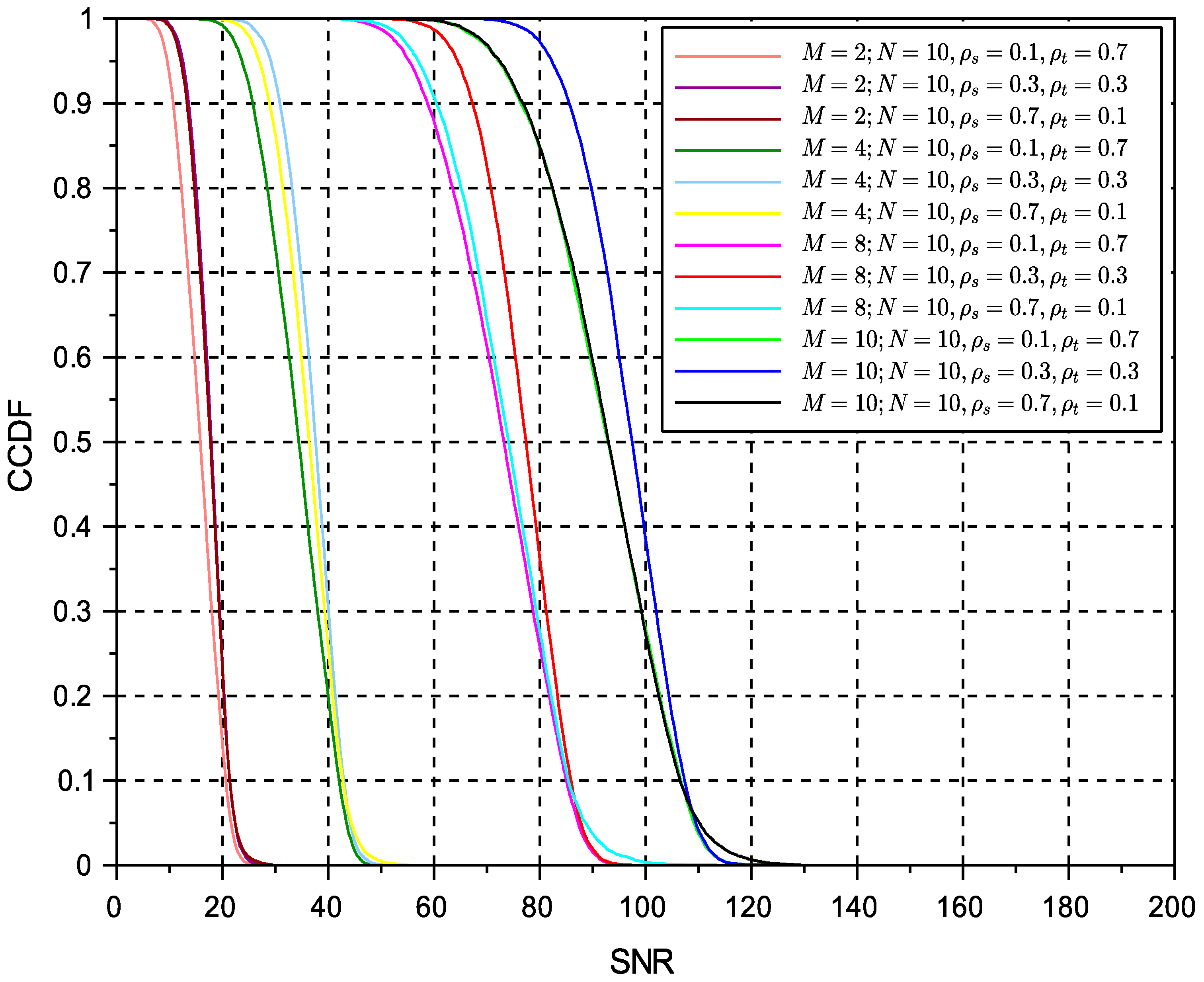
The results in Figure 8 show the performance of the reception statistics where the temporal components are triggered by an SNR threshold, as described in Section 4.5. The simulation considers an activation threshold of $\beta =\gamma MN$, which is equal to the amount of wireless resources being combined weighted by the average signal power. This threshold selection allows us to explore the activation of temporal components with a visible performance, while being a realistic threshold that on average measures a power level of 0 dB for the total number of resources. The results with an activation threshold show a CCDF performance that has a tail behavior that is worse than the results of the previous figure. This is because of the activation threshold being set to a specific value. However, the lack of performance is compensated by the fact that time diversity is adaptive and it is only activated when it is really necessary. This means that in reality the adaptive scheme utilizes less time slots and less resources to transmit information with a given quality, even if the MRC post processing SNR seems to be worse.

6. Conclusions

This paper has presented a space-time correlation performance model for MRC receivers, where branches also occupy the signals received in different time slots. The correlation model provides theoretical expressions assuming equivalent correlation in the time domain (${\rho }_t$) as well as in the space domain (${\rho }_s$). The results of the statistical distribution of the post processing SNR highlight the properties of having two dimensions of equivalent correlation. The results point to interesting conclusions of the behaviour of MRC receivers: at low SNR, higher correlation tends to perform relatively better, while high correlation behaves better in high SNR environments. The two-dimensional MRC processing with adaptive temporal activation presents a few different issues from the fixed time slot MRC processing approach, in general reducing the low SNR behavior with high correlated values. The results with an activation threshold of the temporal components show a worsening effect on the tail distribution of the CCDF of the post processing SNR. However, this relative loss is compensated by the fact of being an adaptive temporal diversity algorithm. This means that resources in the time domain are utilized more efficiently.

The methodology proposed to obtain the statistics of the SNR of the space-time MRC receiver allows us to avoid complex infinite summations that are obtained using conventional methods over the PDF of the random variables. The proposed frequency domain allows us to reformulate the solution as a polynomial root problem. Numerical methods can be used to obtain such roots and do an exact back transform for the resulting PDF. Therefore, the proposed methodology produces exact solutions that do not necessarily rely on infinite summations, which can reduce the complexity of simulation for wireless networks. The only complexity required in this solution is the polynomial root solution, which can be conducted offline if we are dealing with a network with slow mobility patterns.

References

- Sisinni, E.; Saifullah, A.; Han, S.; Jennehag, U.; Gidlund, M. Industrial Internet of Things: Challenges, Opportunities, and Directions. IEEE Trans. Ind. Inform. 2018, 14, 4724–4734. [Google Scholar] [CrossRef]
- Xu, H.; Yu, W.; Griffith, D.; Golmie, N. A Survey on Industrial Internet of Things: A Cyber-Physical Systems Perspective. IEEE Access 2018, 6, 78238–78259. [Google Scholar] [CrossRef]
- Ferrari, P.; Flammini, A.; Sisinni, E.; Rinaldi, S.; Brandão, D.; Rocha, M.S. Delay Estimation of Industrial IoT Applications Based on Messaging Protocols. IEEE Trans. Instrum. Meas. 2018, 67, 2188–2199. [Google Scholar] [CrossRef]
- Bai, L.; Wang, C.X.; Wu, S.; Lopez, C.F.; Gao, X.; Zhang, W.; Liu, Y. Performance comparison of six massive MIMO channel models. In Proceedings of the 2017 IEEE/CIC International Conference on Communications in China (ICCC), Qingdao, China, 22–24 October 2017; pp. 1–5. [Google Scholar] [CrossRef]
- Lu, L.; Li, G.Y.; Swindlehurst, A.L.; Ashikhmin, A.; Zhang, R. An Overview of Massive MIMO: Benefits and Challenges. IEEE J-STSP 2014, 8, 742–758. [Google Scholar] [CrossRef]
- Ghosh, A.; Maeder, A.; Baker, M.; Chandramouli, D. 5G Evolution: A View on 5G Cellular Technology Beyond 3GPP Release 15. IEEE Access 2019, 7, 127639–127651. [Google Scholar] [CrossRef]
- Dietrich, F.A.; Utschick, W. Maximum ratio combining of correlated Rayleigh fading channels with imperfect channel knowledge. IEEE Commun. Lett. 2003, 7, 419–421. [Google Scholar] [CrossRef]
- Ma, Y.; Schober, R.; Pasupathy, S. Effect of channel estimation errors on MRC diversity in Rician fading channels. IEEE Trans. Veh. Technol. 2005, 54, 2137–2142. [Google Scholar] [CrossRef]
- Samano-Robles, R.; Lavendelis, E.; Tovar, E. Performance Analysis of MRC Receivers with Adaptive Modulation and Coding in Rayleigh Fading Correlated Channels with Imperfect CSIT. IEEE Trans. Veh. Technol. 2016, 2016, 6940368. [Google Scholar] [CrossRef] [Green Version]
- Bithas, P.; Maliatsos, K.; Kanatas, A. The bivariate double Rayleigh distribution for multichannel time-varying systems. IEEE Wirel. Commun. Lett. 2019. [Google Scholar] [CrossRef]
- Ma, Y. Impact of correlated diversity branches in Rician fading channels. In Proceedings of the IEEE International Conference on Communications, Seoul, Korea, 16–20 May 2005; Volume 1, pp. 473–477. [Google Scholar]
- Hui, H.T. The performance of the maximum ratio combining method in correlated Rician-Fading channels for antenna-diversity signal combining. IEEE Trans. Antennas Propag. 2009, 53, 958–964. [Google Scholar] [CrossRef]
- Loskot, P.; Beaulieu, N.C. A unified approach to computing error probabilities of diversity combining schemes over correlated fading channels. IEEE Trans. Commun. 2009, 57, 2031–2041. [Google Scholar] [CrossRef]
- Beauliu, N.C.; Zhang, X. On selecting the number of receiver diversity antennas in Ricean fading cochannel interference. In Proceedings of the IEEE Global Telecommunications Conference (Globecom), San Francisco, CA, USA, 27 November–1 December 2006; pp. 1–6. [Google Scholar]
- Beauliu, N.C.; Zhang, X. On the maximum number of receiver diversity antennas that can be usefully deployed in a cochannel interference dominated environment. IEEE Trans. Signal Process. 2007, 55, 3349–3359. [Google Scholar] [CrossRef]
- Beauliu, N.C.; Zhang, X. On the maximum useful number of receiver antennas for MRC diversity in cochannel interference and noise. In Proceedings of the 2007 IEEE International Conference on Communications, Glasgow, UK, 24–28 June 2007; pp. 5103–5108. [Google Scholar] [CrossRef]
- Dong, Y.; Hughes, B.L.; Lazzi, G. Performance analysis of maximum ratio combining with imperfect channel estimation in the presence of cochannel interferences. IEEE Trans. Wirel. Commun. 2009, 8, 1080–1085. [Google Scholar]
- Le, K.N. A review of selection combining receivers over correlated Rician fading. In Digital Signal Processing; Elsevier: Amsterdam, The Netherlands, 2019; Volume 88, pp. 1–22. [Google Scholar]
- Samano-Robles, R. Joint Beamforming, Terminal Scheduling, and Adaptive Modulation with Imperfect CSIT in Rice Fading Correlated Channels with non-persistent Co-channel Interference. IJATES 2017, 10, 186–195. [Google Scholar]
- Hemachandra, K.T.; Beaulieu, N.C. Novel representations for the equicorrelated multivariate non-central chi-square distribution and applications to MIMO systems in correlated Rician fading. IEEE Trans. Commun. 2011, 59, 2349–2354. [Google Scholar] [CrossRef]
- Beaulieu, N.C.; Hemachandra, K.T. Novel simple representations for Gaussian class multivariate distributions with generalized correlation. IEEE Trans. Inf. Theory 2011, 57, 8072–8083. [Google Scholar] [CrossRef]
- Samano-Robles, R.; Lavendelis, E. Performance model for MRC receivers with adaptive modulation and coding in Rayleigh fading correlated channels with imperfect CSIT. In Proceedings of the 2015 Advances in Wireless and Optical Communications (RTUWO), Riga, Latvia, 5–6 November 2015; pp. 26–29. [Google Scholar]
- Samano-Robles, R.; Gameiro, A. A performance model for maximum ratio combining receivers with adaptive modulation and coding in Rice fading correlated channels. In Proceedings of the 2014 IEEE Symposium on Computers and Communications (ISCC), Funchal, Portugal, 23–26 June 2014; pp. 1–6. [Google Scholar]
- Karagiannidis, G.K.; Zogas, D.A.; Kotsopoulos, S.A. On the multivariate Nakagami-mdistribution with exponential correlation. IEEE Trans. Commun. 2003, 51, 1240–1244. [Google Scholar] [CrossRef] [Green Version]
Figure 1.
Multiple antenna receiver system.
Figure 2.
Maximum ratio combining receiver.
Figure 3.
Equal gain combining receiver.
Figure 4.
Methodologies for calculation of statistics of correlated MRC receivers.
Figure 5.
Maximum ratio combining receiver in space and time.
Figure 6.
Methodology to calculate statistical functions based on transforms.
Figure 7.
CCDF of the instantaneous SNR for different values of spatial and temporal correlation coefficients and number of antennas of the MRC receiver.
Figure 8.
CCDF of the instantaneous SNR conditional on for different values of spatial and temporal correlation coefficients and number of antennas of the MRC receiver.