Waiter Robots Conveying Drinks
by
Ash Yaw Sang Wan
1, 
Yi De Soong
1,
Edwin Foo
2,
Wai Leong Eugene Wong
3 and
Wai Shing Michael Lau
3,* 1
Singapore Institute of Technology @NYP, Newcastle University, Singapore S567739, Singapore
2
Nanyang Polytechnic, Ang Mo Kio, Singapore S569830, Singapore
3
@NewRIIS, Newcastle University, Singapore 609607, Singapore
*
Author to whom correspondence should be addressed.
Technologies 2020, 8(3), 44; https://0-doi-org.brum.beds.ac.uk/10.3390/technologies8030044
Submission received: 2 July 2020
/
Revised: 1 August 2020
/
Accepted: 6 August 2020
/
Published: 11 August 2020
Abstract
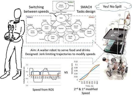
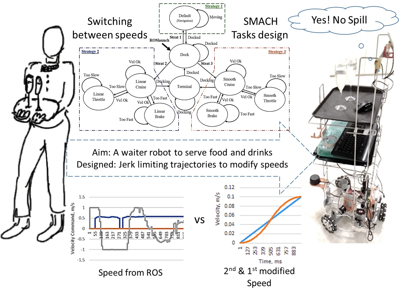
:Robots have been reportedly seen serving food in several restaurants in many parts of the world. New ventures have been deploying mechanical partners which promote the growth in service robotics. However, robots are considerably incompetent when it comes to beverage and soup delivery. The physical challenge behind the clumsy motion of these machines is found to be its jerky motion control. Jerk control solutions are widely studied in a constrained environment but not well introduced in dynamic environments. In this paper, we will begin by examining developed kinematics solutions, open-source packages from Robot Operating System and the constraints of motion planning. The proposed solution in this paper provides a quick system response with jerk limits using spline velocity profiles. The solution will introduce the concepts of a state machine design that enables the robot to behave and move reactively; effectively balancing its desired velocity and position without spilling a drop of customer satisfaction. Experiments have proven that robots can move at higher velocity without any crashing, spilling, or docking issues. The smooth velocity control proposed will improve the capabilities of waiter robot and service operations in restaurants.
1. Introduction
1.1. Waiter Robots in Food and Beverage (F&B) Industry
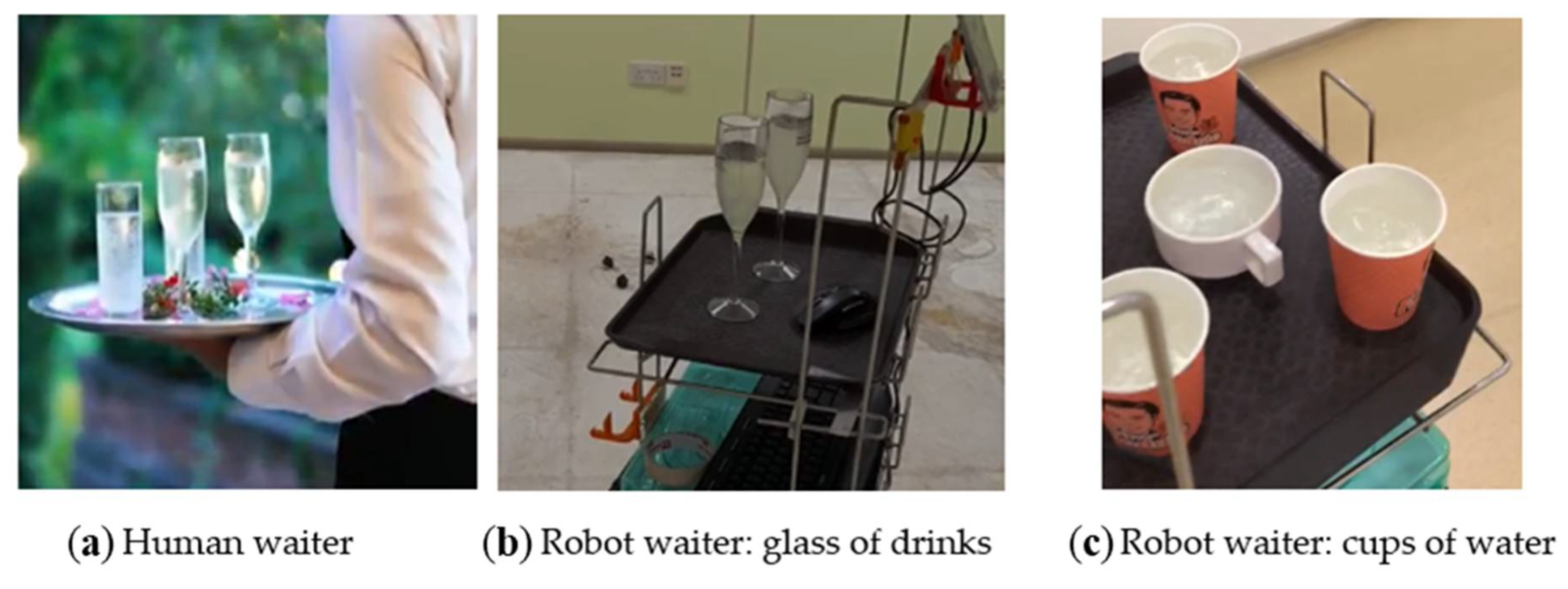
The manufacturing sectors have been integrating robots into their operations and improving their productivities for many years. On the other hand, robots in the service sector are just picking up and expected to grow [1] after initial mixed successes: replacing workers [2] and being replaced themselves [3], in China. Similar initial mixed experience in Singapore: Pin Xian Lou restaurant [4] introduced its humanoid waiter robots in 2017 but the novelty and appeal to children soon wore out. Additionally, the robot meandered its way along a guided path and unable to serve food directly to the tables. New ventures with robots grew in more restaurants in India [5,6], Hungary [7], and Nepal [8] with robots delivering food to diners; and it inevitably will as robotics designs and algorithms get better. Yet, the great challenge of waiter robots is to deliver beverages and soups filled to the normal level (Figure 1).
Besides drinks and beverages, there are soups and broth to be delivered. Chinese restaurants serving hot pots, very popular among Asians, may have robots serving dishes but the hot soups are still carried to the table by waiters, or as observed in some restaurants, half-filled drinks served in plastic cups.
In this paper, we will address this issue of waiter robots conveying standard liquid-filled glasses, and cups. This is done first by examining the standard motion control routines in ROS for a mobile robot, understanding what causes spills and experimenting with velocity profiles used in industrial robots. Typically, most robot-controlled motions are either discrete square wave signals or signals with ramp transitions [9,10,11]. Most program strategies only consider the computation time and direction of motion but do not consider the design and control of jerk constrained motion profiles. This is why waiter robots are not commonly deployed to deliver liquids (i.e., soups and beverages) in open crockeries. Human waiters in the food and beverage industry are committed to serving drinks, especially in bars and cocktail parties before formal dinner is served. It will be a huge improvement in waiter robot capabilities to glide and weave around guests in cocktail parties. Our results show that it is possible to replicate human capabilities in our waiter robot.
1.2. Robot Motion
The main constraint in most waiter robots delivering liquid-based items to customer tables is the uncontrolled jerk [12]—the derivative of acceleration or the 3rd derivative of position with respect to time. The initial motion of a liquid body is sensitive to jerks—a portion of the body of liquid will be pushed up against the container wall, then the impact and the momentum will move that portion of liquid back to its main body, pushing part of it over to the other side. If liquid moves above the brim of the container, some of it will be spilled. Similar spillage can occur when the robot waiter stops with an uncontrolled jerk. The design of a motion profile with a constraint on the jerk limit can solve the spillage problem. For example, the robotic arms used in manufacturing are programmed to move smoothly. The motion profile is designed with a limit on the jerk.
Macfarlane et al. [13] proposed a methodology that uses the quintic concatenations of sinusoidal equations to provide a smooth trajectory for the motion of the robotic manipulator between two way-points. In another paper, Vass et al. [14] suggested a near time-optimal trajectory executor algorithm. The paper mentioned that reducing jerk is necessary to avoid vibrations and the wear and tear of mechanical components of the robot. The algorithm is improved and redeveloped from the minimum-time spline-based reduced state space approach (MSRS). The disadvantage of MSRS is the lack of flexible control because of its requirement to obtain a steady velocity at the end of each spline. The researchers continued from MSRS approach and had successfully reduced the robot motion computation time to 100 ms.
In 2006, Huang et al. used Genetic Algorithm, GA [15] to design a trajectory to reduce jerk motions for space robots. In 2010, Pattacini et al. developed a Cartesian controller which extends the multi-referential dynamical system approach [16] to enhance the smoothness, the speed, the repeatability, and the robustness of the robot motion. The approach combined the use of a joint-space and task-space controller via the use of Lagrangian multipliers methods to modulate the output of each function. The cascaded controllers are used to replace the vector-integration-to-endpoint models. HI Lin [17] argued that the previous methods were time-consuming because of the complicated procedures involved and proposed a fast and unified method using particle swarm optimization. Zhao et al. [18] used a third-degree polynomial function to describe trajectories of service manipulator robots and proposed a quick algorithm that operates with configured motion in state space. The solution is able to generate a piecewise straight-line trajectory that is bounded in jerk, acceleration, and velocity. The solution also included removing unnecessary motion to smoothen the path. The computation time requires 1.1 s which generates a natural-looking motion using the Kuka light-weight robot IV.
These various concepts in handling jerk motion profiles can solve the problem of jerky motion in robots but have complicated procedures and are computationally intensive. The motion planners can achieve their tasks well as these robots are fixed manipulators operating in a well-constrained environment. Waiter robots, on the other hand, do not have the same luxury of a static surrounding and hence require a quicker processing logic or reactive behaviors. At the same time, a mobile robot may be required to make sharp turns in the presence of dynamic obstacles, disrupting the planned smoothen path.
For mobile robotics applications, Park et al. [19] mentioned that to achieve comfort for users on a robotic wheelchair, the dynamic-window-approach and vector field histogram (DWA and VFH) are not suitable for such applications. Implying that jerk motions are not well controlled for the needs of the users. To obtain a smoother and graceful motion, they have developed a reactive behavioral method using a heterogeneous control and human-like driving strategy. Korayem et al. [20] developed a computational algorithm for a 3-wheeled mobile manipulator. According to the paper, jerks also contribute to the slippage of wheels. The paper proposed a hybrid approach adapting a time-optimal path planning [21] and the potential field method for obstacle avoidance [22].
From the review above, the need to manage the jerk to provide a smooth motion has been made. However, the methods found in the literature are quite computation intensive even for a static environment. In this research work, this paper proposed a simpler approach for designing the motion profile with jerk limits. To cater for different load condition, a state machine algorithm is proposed to manipulate the kinematic motions of a waiter robot using different appropriate profiles depending on the load. It uses simple and reactive control methods to enable reactive motion behaviors. It is developed in the robot operating system environment for a 3-wheeled omni-directional waiter robot designed for casual dining restaurants presented previously by Wan et al. [23].
2. Analyzing the Root Problem
2.1. Velocity from ROS Navigation Package
The open-sourced platform robot operating system (ROS) have libraries for navigation and velocity control of a mobile motion. This section will first discuss the velocity control routine from the ROS navigation package, other routines such as, “yujin velocity smoother,” “joint trajectory generator,” and lastly the proposed liquid-conveying algorithm, developed using “SMACH”—a ROS Python package.
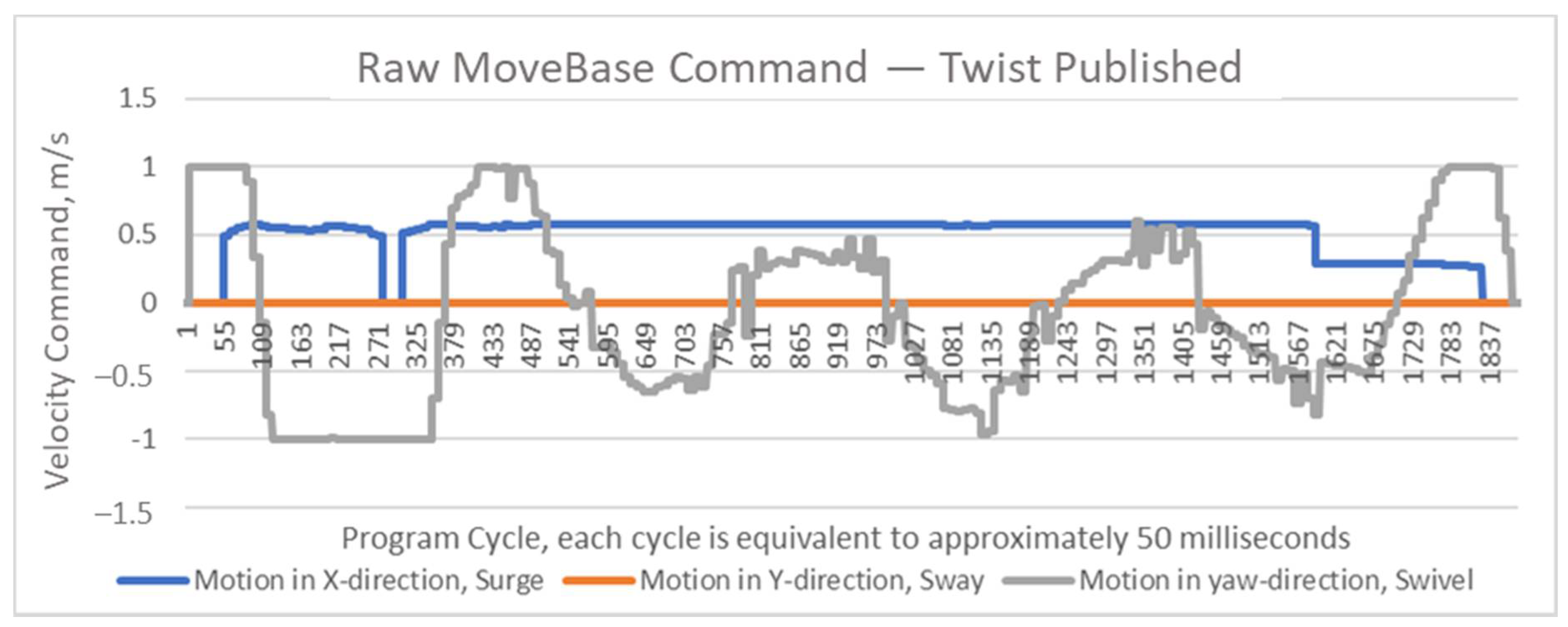
The ROS navigation stack uses odometry calculations, sensor inputs and moves base scripts to generate a twist profile. In ROS, a twist is a sort of class in programming that holds linear and angular velocity values. The navigation stack generates ways-points and the move base node generates velocity commands relative to the robot also known as a twist.
A typical twist generates step velocity profiles, as shown in Figure 2, for robot motion in the x, y, and yaw directions. These voltages are distributed by a user-developed node to the respective motors.
The step voltages depending on the magnitudes, may result in high jerk motions during start and stop. There are online packages to smoothen the velocity profiles generated from the navigation stack. The “yujin velocity smoother” [10] and “joint trajectory generator” [11] are examples that smoothen the velocity profile using pre-set acceleration limits. The smoothened generator produces velocity commands based on the maximum allowable acceleration value resulting in smaller velocity steps being generated as speed commands to the wheels. By generating smaller steps and converting step-up and step-down velocity into a sequence of smaller step-up/step-down velocity profile, a form a velocity smoothening is produced. Effectively, the profile will reduce the magnitude of motion jerks.
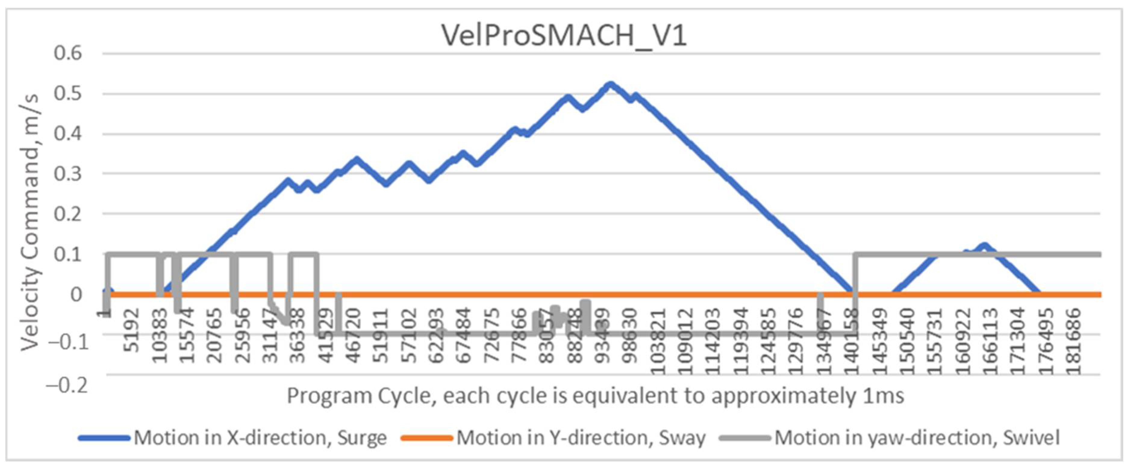
Using a similar approach, a ramp-velocity profile generator is designed—the acceleration or the gradient of the ramp can be programmed to produce a smoother start and stop motion. This has been coded using the state machine python script (SMACH [24]) and named VelProSMACH_V1.py. It generates a velocity profile illustrated in Figure 3. The reason for using SMACH will be made clearer when a robotic behavior algorithm is designed to switch among the ROS navigation package-generated step-velocity profile, the ramp-velocity profile, and to be introduced, the S-velocity profile.
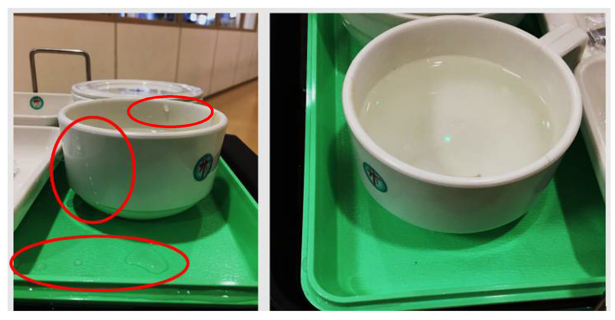
The performance of the two types of velocity profiles was tested on an in-house developed waiter robot [23]: step-up or step-down velocity from ROS navigation move base and the ramp-up or ramp-down velocity profile from VelProSMACH_V1.py. The robot conveyed water in cups along a straight line from Point A to Point B, repeated ten times. The difference in spillage for cups (the left diagram with droplets along the outside and the inside of the cup and on the tray) due to robot motions generated by the two motion profiles are shown in Figure 4.
VelProSMACH_V1 had achieved satisfactory performance for general motion but is not desirable for restaurant setting because of its inability to track waypoints along the trajectory or for accurate docking. The robot was observed to bumping into walls and obstacles because of its late response and oscillatory motion about the docking location before coming to a stop.
This suggests a possibility for improvement in waiter robot tasks. However, there is a trade-off.
2.2. Stability Versus Docking
To minimize minimum or zero spillage, control of the instantaneous change from initial speed up to the desired speed requires a gentle ramp change in velocity. This, however, will cause the waiter robot to react slowly toward any change: it may not be able to change its direction quickly, and may not be able to stop on time. Near the target, the robot decelerates slowly and comes to a stop, often before reaching the target. The distance error will cause the robot to accelerate again and sometimes overshoots the desired point. This can be repeated a couple of times resulting in the robot oscillating about the target point, lengthening the time to reach the target and dock. The docking fails.
The results in Table 1 show the performance using a gentle velocity ramp profile (rate of acceleration at 0.0001 m/s2) for VelProSMACH_V1.py. All the test run from Table 1 have zero incidences of liquid spillage but are unable to accurately dock at the final destination.
If the ramp velocity profile is made steeper, the incidence of liquid spilling increases. However, tuning the ramp slope steeper makes it more responsive and achieves a higher docking success rate. Unfortunately, when the ramp profile is configured with a lower change in velocity, the robot will be able to move without spilling the drinks carried but it is maneuvering as if with high inertia of motion. Trading off between motion smoothness and docking accuracy with a cap on the jerk limit is difficult, many times it is a hit and miss situation. This will be useful when the waiter robot delivers food instead of fluidic items. It will have sufficient reaction time to respond to changes in the path trajectories. The robot start and end motion will be smoother than those generated by the step velocity profile.
The move base step velocity profile, on the other hand, is used successfully for autonomous motion in point to point navigation and in docking. It has, however, high starting accelerations and ending decelerations that can cause drinks to spill from some tall glass (e.g., a champagne glass), if not secured.
Robots have to be able to move smoothly and quickly for efficient utilization. Neither the step nor the linear velocity profile is able to resolve the motion issues of conveying drinks as liquid bodies are sensitive to the jerk instead of acceleration. A changing rate of acceleration will be required for the robot motion to be both smooth and quick; a low level and constant jerk process should be imposed.
2.3. The S-Velocity Profile
The spline velocity or S-velocity profile commonly used in robot manipulator trajectory changes the speed more gently, with the maximum acceleration at the instance of transiting from the concave to the convex part of the velocity profile. In this paper, the spline velocity motion profile has been investigated with simple computation approach.
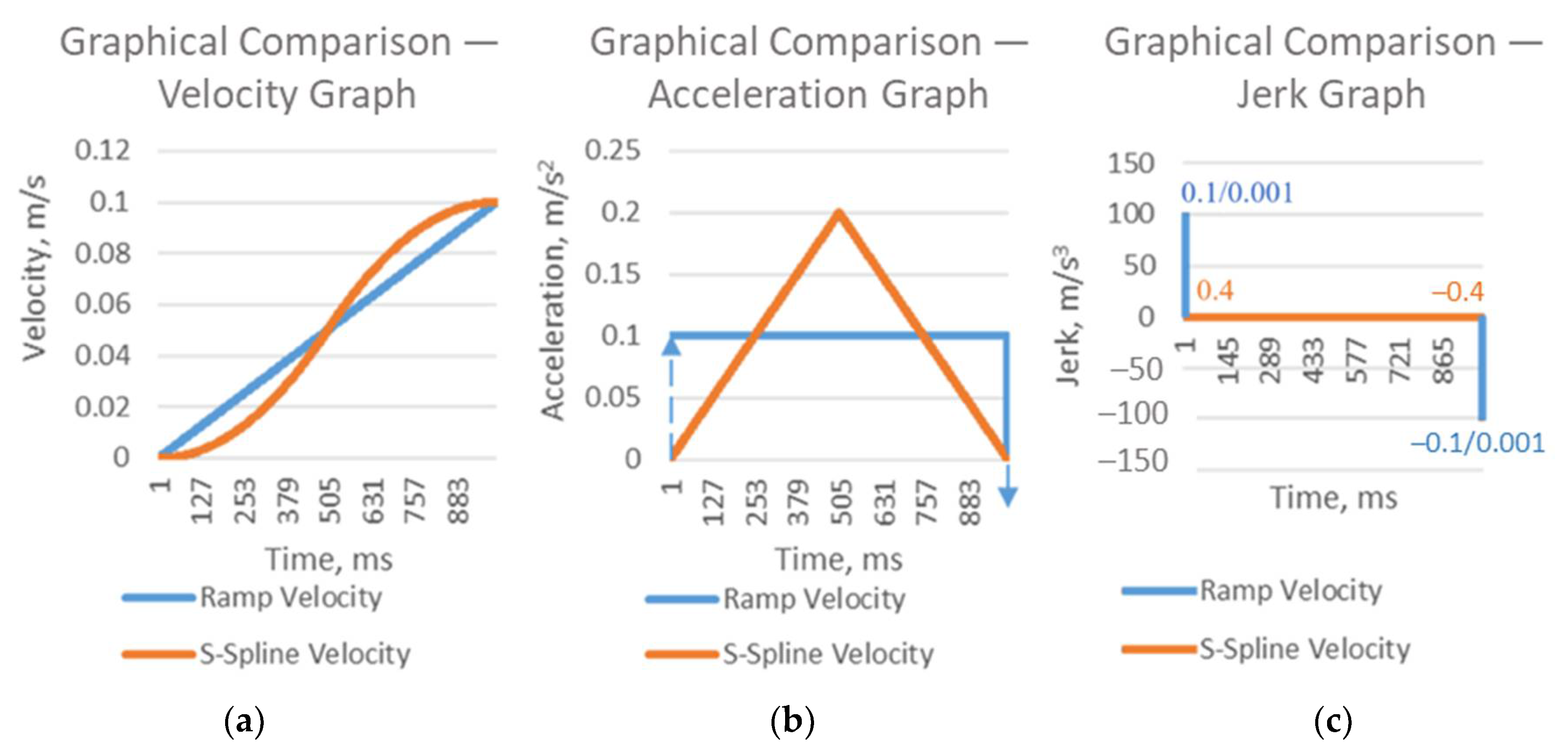
Figure 5 shows a ramp-velocity that changes from 0 to 0.1 m/s in 1 s, sampled at 1 ms interval with an impulsive jerk magnitude of 100 m/s3. In comparison, the speed change of the S-velocity curve, over the same period, is smoother; more importantly the acceleration increases at a steady rate leading to a smaller constant jerk magnitude of 0.4 m/s3 and then to −0.4 m/s3. Potentially quicker system response with lower jerk levels is achievable and will enable the waiter robot to start (and stop) smoothly without introducing severe jerk to the liquid in the glass or cup.
The S-velocity curve can be generated using a set of kinematic equations with at least a cubic, or higher fifth-order polynomials, otherwise using a sinusoidal function. Many papers were written on optimization and solving the coefficients of such polynomials as discussed earlier. The approach taken here is based on experimentation with different types of liquid containers and the S-velocity profile is hardcoded in Python using the value increment operations.
Equations (1) and (2) are the velocity and acceleration generators for the S-curve. The change in velocity, for each time step, is given by:
where refers to the current velocity command
refers to the previous velocity command
refers to change in velocity command
The change in acceleration, for each time step, is given by:
refers to change in velocity command
where sgn(j) = 1 for the concave part of the S-Curve
and sgn(j) = −1 for the convex part of the S-Curve
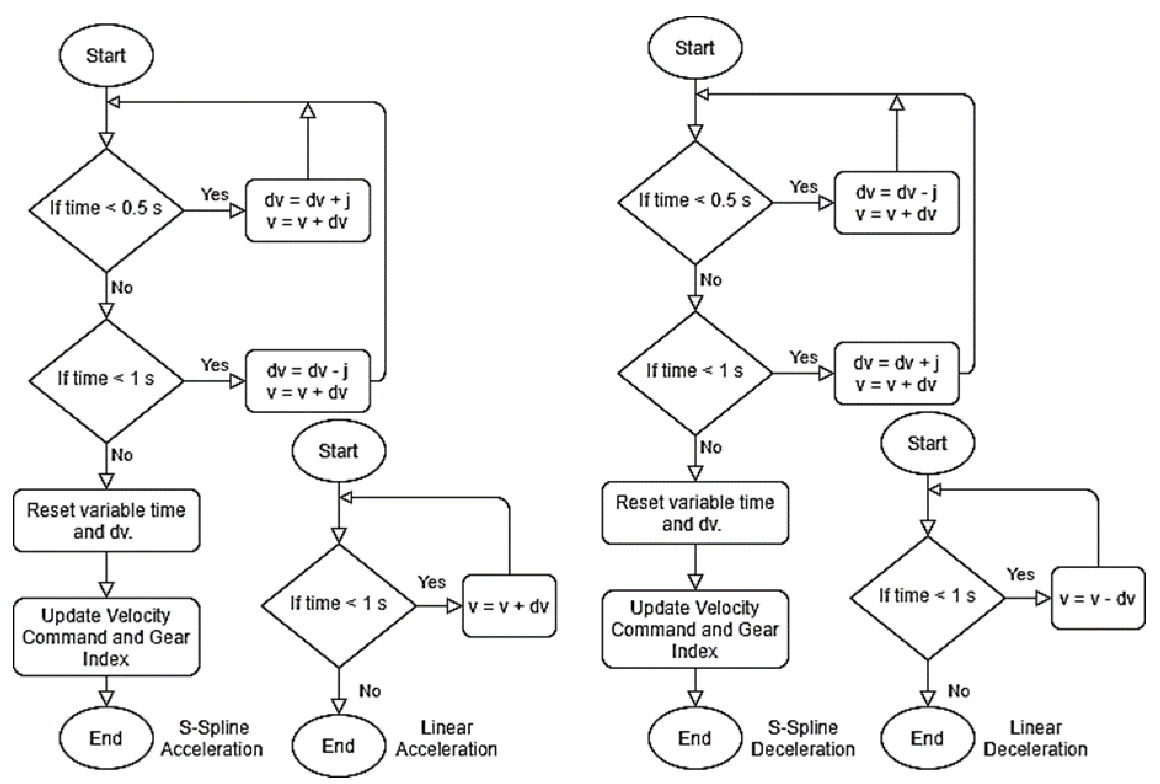
When the robot is to accelerate, sgn(j) equals to 1, (1) and (2) are used to generate the concave part of the speed profile. After 0.5 s, the robot speed will switch into the convex part of S-speed using (1) and (2), sgn(j) equals to −1. The variables will be reset once acceleration/deceleration is completed (reaching the desired velocity). The ramp-velocity and the S-velocity flow charts are shown in Figure 6.
To compute at a lower rate, a loop counter is applied to model the time discretization using basic delays and counters. Assume transition time of 0.5 s to peak acceleration and publish command every 1 ms. The transitional time value is determined experimentally through calibration and tuning of the robot configuration. This is performed based on the reaction time required in general to react to obstacles in close-proximity (when obstacles are equal or less than 0.2 m away) while travelling at 0.1 m/s. The travelling velocity of the robot is relatively low as it is also expected to navigate through tight space in a typical restaurant environment. Hence, the time response of the transient velocity is benchmarked at 1 s.
3. Designing the Waiter Robot Motion Behaviors—VelProSMACH_V2.py
The utility of a waiter robot increases if it is able to move normally without load, transit to moving slowly and safely when carrying drinks or food, in the same way, a waiter does and then transiting back to moving normally once the food or drinks have been delivered [25]. Each of the three velocity profiles experimented with can be regarded as a type of behavior: step-velocity profile as moving with no tray (normal robot point-to-point motion), ramp-velocity profile with carrying food tray, and S-velocity profile with carrying food with drink trays. A complex waiter robot behavior can result in an unexpected situation from these motion profiles. Different states of motion control can be used in various scenarios.
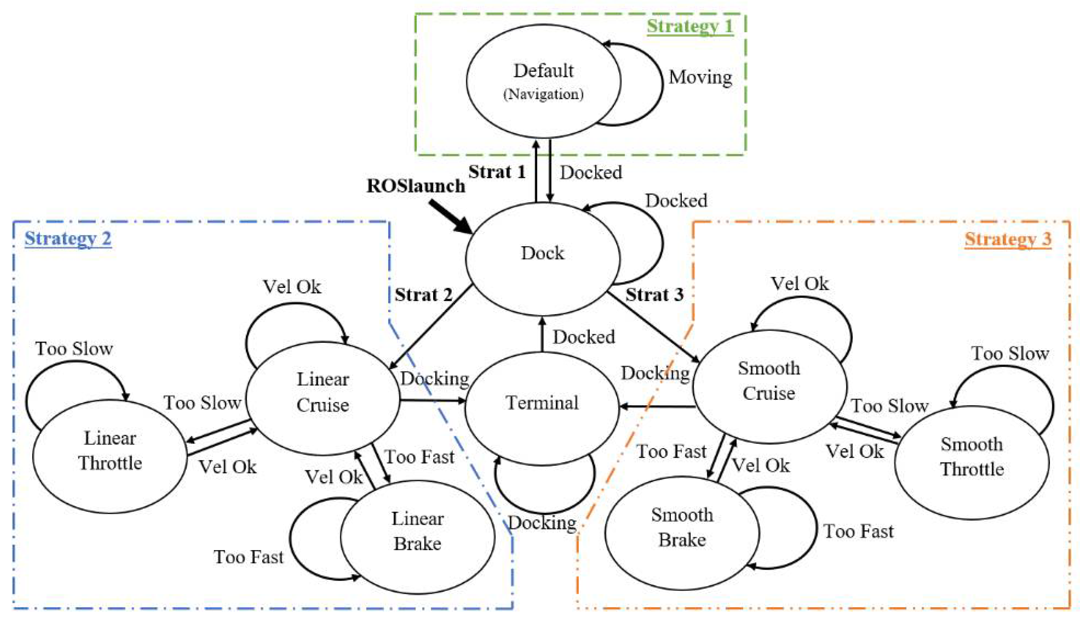
A convenient tool for prototyping and developing the waiter robot with suitable motion behaviors and transiting between these motion states is the ROS SMACH package. It is a task-level architecture for rapidly creating basic and complex robot behaviors. In ROS, the state machine can be used to generate sensible twist commands for waiter bots in restaurants. VelProSMACH_V2.py is the implementation of the state machines for the waiter robot. The state machine diagram is shown in Figure 7.
3.1. Motion Behavioral Strategies
The state machine is designed to link the “linguistic” outcomes to different states. These outcomes can be designed as event handlers to transit into discrete states under various circumstances. The “Dock” state is the interface to ROS navigation node and decisions are made here to nullify the move base commands and switch into other move commands as a motion strategy hub. It may transit to various states depending on the payload e.g., of the food or drinks. For one case, the robot would move with the S-velocity profile while carrying drinks to a table, then subsequently deliver the remaining food with a ramp velocity profile and then return to the start point with step velocity profile (the default state which uses the navigation move base command). This Dock state is effective and ideal for the robot to deal with various tasks appropriately and semantically. The change of motion strategy is likely to optimize businesses’ operation efficiencies.
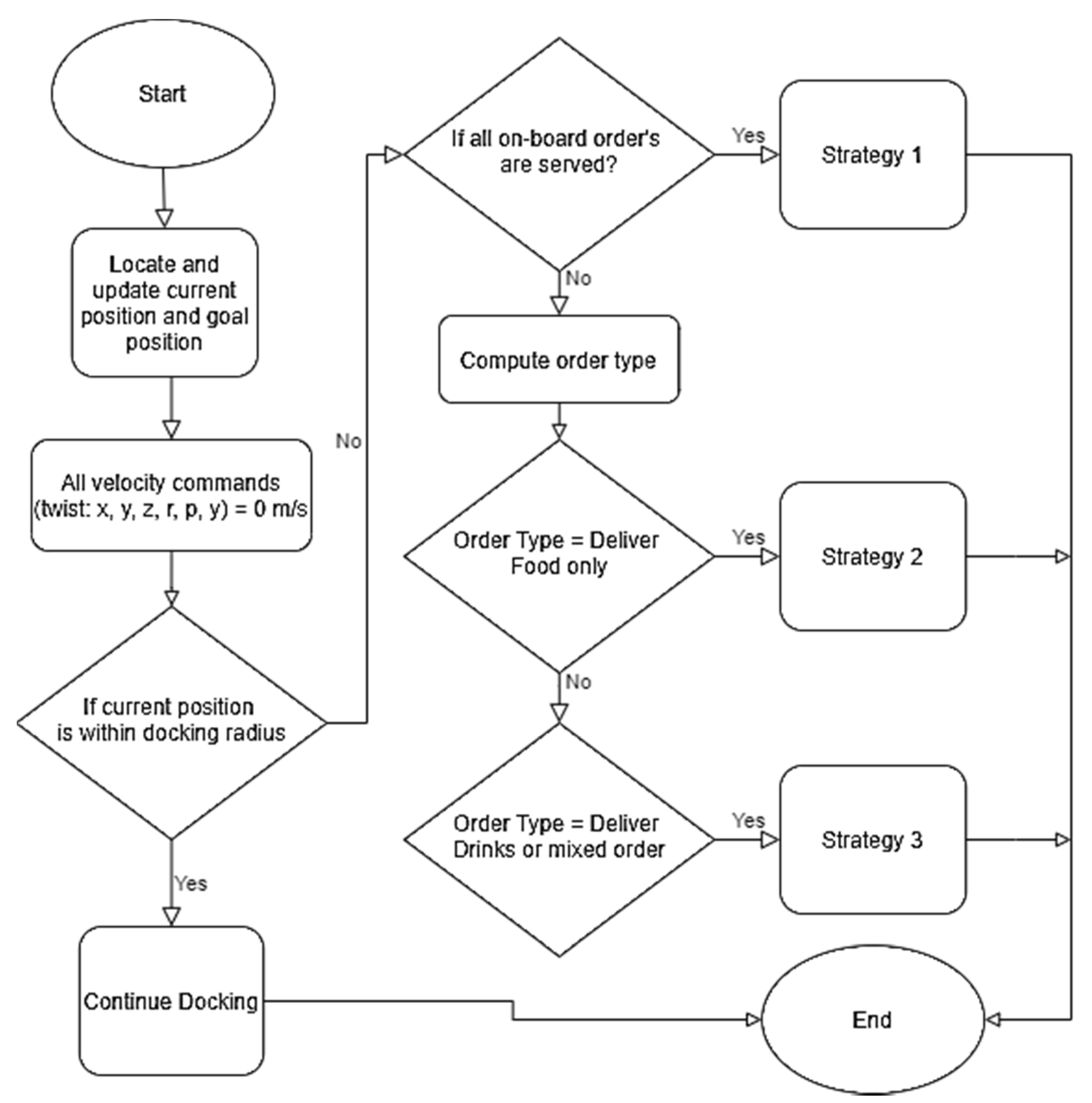
The decision to switch between strategies depends on the food order (the task of the robot). The robot is expected to use the appropriate motion strategies to maneuver effectively and efficiently based on the task on hand. This is currently done from the terminal but it can be implemented using a set of manual push buttons on the robot, for the various type of load, as inputs to the robot controller. An ordering system developed from a previous prototype, the Beta-G [26] can also be integrated: when the food is ready, the ordering system should indicate the table number and the type of order ready to be served; solid food to be using Strategy 2 while liquid and semi-liquid food to be on Strategy 3. When returning to a waiting position in the restaurant, the robot transits back into Strategy 1. The program flowchart of the dock state for motion strategy switching mechanism is shown in Figure 8.
A concept of a motion state transition hub may be programmed and enforced. The respective “Cruise” states enable the robot to switch its motion state by deciding whether to increase or decrease its speeds. The state can also choose to remain on its current state; to maintain speed in the same direction. Each motion strategy transits reactively based on the current speed, the remaining distance to the goal or obstacles. Note that this is only an example of how the SMACH can be used to enable the use of simple value increment code.
3.2. Reactive and Non-Reactive States for a Multispeed Design
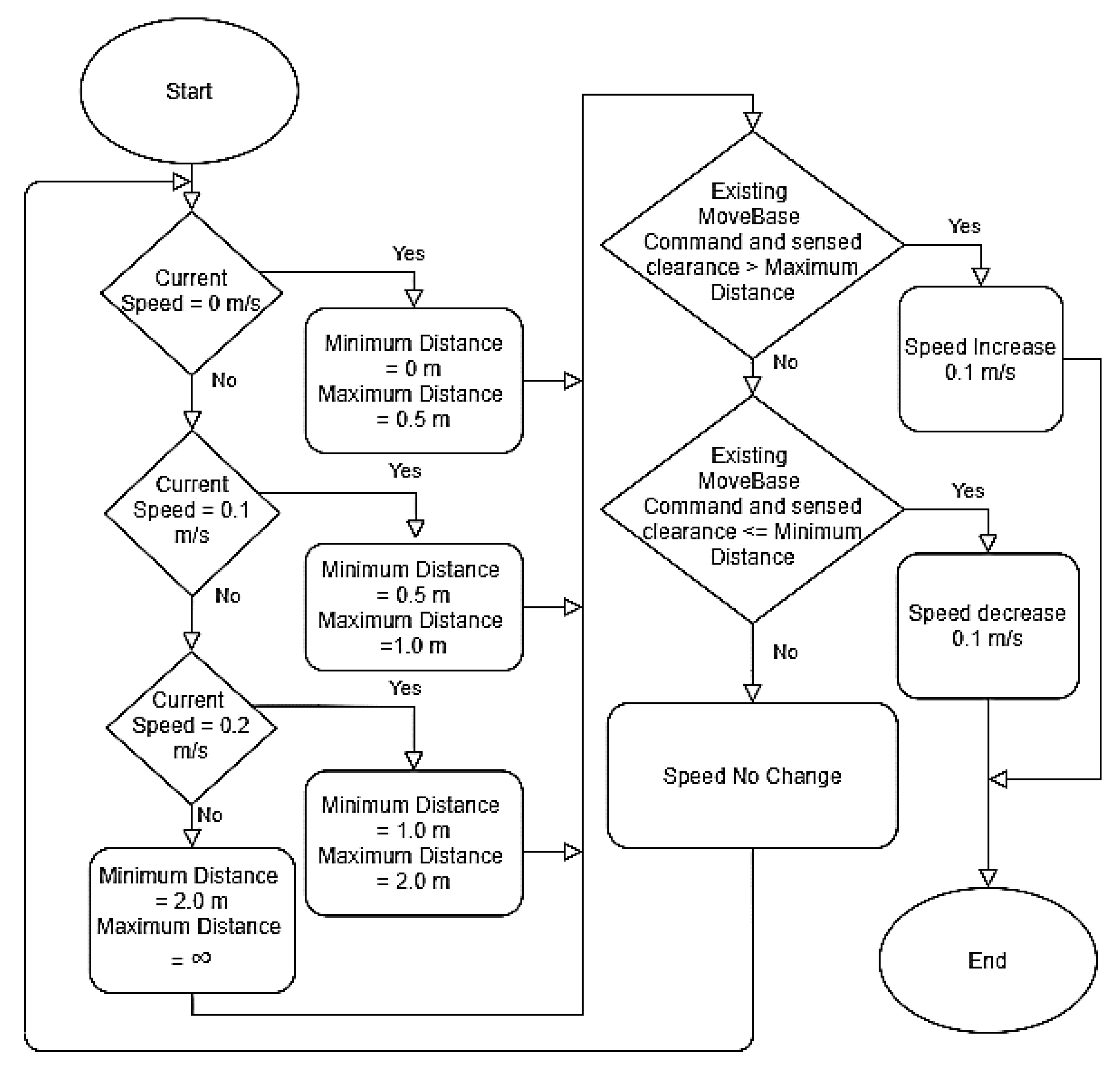
The cruise state requires and generates low discretization of desired speed (i.e., 0.1, 0.2, and 0.3 m/s) and current speed system level. The desired speed changes are based on scenario logic. The logic compares move base commands, Adaptive Monte Carlo Localization position (AMCL pose) inputs, and its current velocity state. By determining the targeted velocity and acting on current velocity values and position, it allows the robot to cruise at the desired velocity. As restaurant areas are usually spatially tight, the cruise state will allow the robot to manage its motion around obstacles better. The program flowchart of the cruise state is shown in Figure 9.
The robot’s reactive cruise state depends on whether or not the move base provides a twist command. With a twist command and the goal position, the robot will increase speed (throttle) toward a higher speed. Likewise, when the robot’s goal position or if an obstacle is near, the robot reduces speed (brake). The robot motion is designed in the same way as humans drive their cars. When other cars or obstacles are near, the vehicle is slowed down and once past these, the vehicle speeds up. The same logic can be applied when the robot is navigating a bend. The robot speed is feedbacked by speed encoders on board.
The throttle and brake states in S-velocity are used to generate linear acceleration and linear deceleration. A constant loop period and a defined change in velocity provide an acceleration profile with a consistent jerk magnitude. A counter will begin counting the loop cycles. The loop thresholds are also set to maintain the magnitude of the maximum acceleration, acceleration period, and outcome velocity. Note that the smooth throttle and smooth brake states will not be interrupted or transit into other states during the acceleration period; this means that the period determines the time response of the robot before it can decide to vary its speed. The higher the loop threshold, the longer it takes for the robots to the response. For this motion behavior, the states are non-reactive. The robot will only be reactive again after the completion of the S-velocity profile. Unlike the S-velocity profile, there is no requirement to limit jerk for the robot in step-velocity and ramp-velocity. Hence these motions can remain reactive.
When the robot approaches its goal point, the waiter robot transits into a terminal state where it uses small step-up and step-down velocities to reach the docking point as accurate as possible.
4. Comparing ROS Step-Velocity and S-Velocity
Tests were done with the waiter robot conveying water in cups and champagne glasses running under ROS navigation node base commands issuing step-velocity commands and the developed VelProSMACH_V2.py running in the S-velocity mode. The cups and glasses experiments are done separately. The goal position is approximately 5 m away from the start position. The waiter robot was set to run 20 times. The cups and glasses are filled with water until the 1st finger joint from the brim.
Results
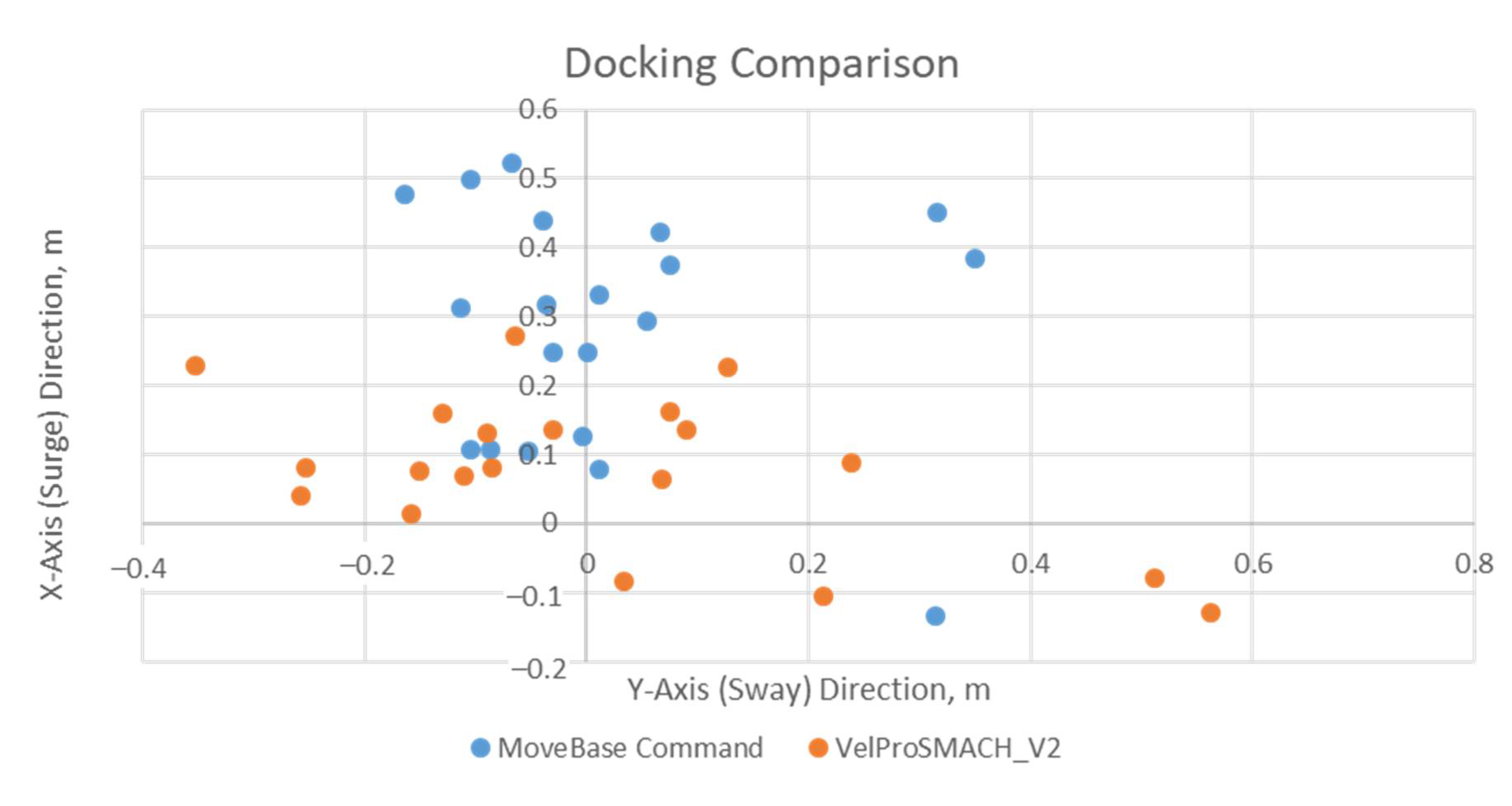
Figure 10 shows a comparison of docking accuracy. There are no distinct differences between the two algorithms, although the waiter robot seemed to be docking slightly more accurately toward the goal position. The move base command tends to overshoot the docking position in the x-direction.
Table 2 and Table 3 show the specific data for docking and performance in conveying water in cups for the two programs; MoveBase control and VelProSMACH_V2 respectively. The mean docking radius improved from 329.6 mm for the step-velocity to 233.8 mm for the S-velocity, and the docking variance improved from 234.4 mm to 17.8 mm. In addition, the S-velocity profile did not result in any liquid spillage, while the step-velocity resulted in spillage in all 20 runs. However, the S-velocity, in general, took on average one and half time longer to reach its destination. This is to be expected, even for a human waiter as the need to control the motion can slow one’s pace. Results for water in glasses are similar in that there is no spillage; the timing and accuracy are about the same, not identical.
There are some limitations to the use of VelProSMACH programs. The S-velocity profile requires calibration and fine-tuning to obtain the results. This tuning will vary for various mobile robot designs. Debugging and testing of suitable jerk parameters will be one of the key constraints of this motion control design.
Another limitation is the inflexibility of disrupting the S-velocity profile from the smooth throttle or smooth brake state. This results in a longer period for the waiter robot to respond to change its operational plans. This is limited due to the value increment hard coding implementation of the velocity to decelerate numerically with a controlled jerk. This is unlike trajectory planning of industrial robot manipulators where the trajectory is designed in almost a fixed environment.
For safe operation, the ROS motion algorithm in the navigation package has obstacle detection and avoidance behaviors using the LiDAR and a set of eight Teraflex IR sensors arranged around the base of the robot for close proximity sensing. It is designed to be lightweight, open concept, and operates at relatively low speeds. It does not result in a severe impact on collision.
The robot has been successfully tested with both static and dynamic obstacles such as a chair (static) and humans walking toward the robot (dynamic). The collision detection and obstacle avoidance algorithms will slow down the robot with controlled deceleration and does a detour. If a detour could not be done, it will come to a stop when its path is completely blocked.
For additional safety, there is a push-button that when activated removes power from the servomotors. In addition, a set of mechanical bumpers similar to those installed on Beta-G can be implemented.
Finally, the computational time has to be considered. The S-velocity profile requires a discretization time of 1 ms per change in order for the robot to obtain a 1-s reaction (or response) time. To react and to respond faster, the waiter robot requires a finer quantization of time. In cases where the waiter robot on-board computer is required to reduce the command publish rate due to heavy computation requirements by other tasks running concurrently or where the computational power is low by design, the solution proposed here will not be ideal.
5. Conclusions
Robots are seen in restaurants delivering food to the tables, but robots serving drinks and soups, though also part of the basic tasks of waiter are not common. The problem is associated with the jerk in the initial start and stop causing the liquid to spill. With the implementation of the S-velocity profile with a limit in the jerk, it is possible to minimize liquid spillage and to improve on the productivity of waiter robots in the Food and Beverage industry. The S-velocity can be designed into a robotic behavior algorithm, in conjunction with ROS step-velocity and ramp-velocity using state machines tool SMACH ROS. With this, the productivity of waiter robots in the Food and Beverage Industry can increase by assisting in the serving of typical beverages, wine and soups.
Author Contributions
A.Y.S.W. carried out the study of jerk motion experienced by the waiter robot prototype. A.Y.S.W. is the main algorithm developer and tester for program solution mentioned; VelProSMACH_V1 and VelProSMACH_V2. Y.D.S. assisted A.Y.S.W. in this development in coding and experimental data collection. E.F. was the previous developer for the mechatronic and embedded systems of the robot, which includes the Robotis Dynamixel motors and controller used. W.L.E.W. and W.S.M.L. are the main mechanical designers of the waiter robot prototype. Additionally, W.S.M.L. contributed to the derivation of the kinematics control equations used in the robot software. All authors have read and agreed to the published version of the manuscript.
Funding
This research received no external funding.
Acknowledgments
The Waiter Robot team would like to extend their thanks to Steven Tay (Newcastle in Singapore, NUiS) and Lui Woei Wen (Nanyang Polytechnic) for their generous support and technical advises.
Conflicts of Interest
The authors declare no conflict of interest.
References
- MarketWatch. Service Robotics Market US $7.9 Billion Size Expected to Grow at 7% CAGR Forecast Till 2023. 2018. Available online: https://www.marketwatch.com/press-release/service-robotics-market-us-79-billion-size-expected-to-grow-at-7-cagr-forecast-till-2023-supplydemandmarketresearchcom-2019-02-01 (accessed on 22 February 2019).
- AFP/asiaone. Robots Replace Waiters in China Restaurant. 2018. Available online: https://www.asiaone.com/china/robots-replace-waiters-china-restaurant (accessed on 6 August 2018).
- Jen/shanghaiist. Guangzhou Restaurant Fires Its Robot Staff for Their Incompetence. 2018. Available online: https://shanghaiist.com/2016/04/06/restaurant_fires_incompetent_robot_staff/ (accessed on 5 May 2018).
- Lim, K. Meet Robot Waiters Le Le and Xiao Jin at Hot Pot Restaurant Pin Xian Lou. 2017. Available online: https://www.straitstimes.com/lifestyle/food/adding-byte-to-your-appetite (accessed on 8 January 2017).
- The Economic Times. Science City’s Robotic Gallery to soon Serve Food through Robots. 2018. Available online: https://economictimes.indiatimes.com/tech/science-citys-robotic-gallery-to-soon-serve-food-through-robots/robot-waiters/slideshow/66749025.cms (accessed on 22 February 2019).
- Robot Waiters will Serve You at This Restaurant in Coimbatore. 2018, p. 1. Available online: https://www.youtube.com/watch?v=PGYGUUsvtos (accessed on 22 February 2019).
- Lawson, H.; Fenyo, R.K.; Macdonald, L. Robots Serve up Food and Fun in Budapest Café. 2019. Available online: https://www.reuters.com/article/us-hungary-robotcafe/robots-serve-up-food-and-fun-in-budapest-cafe-idUSKCN1PJ1EJ (accessed on 22 February 2019).
- AFP. Nepal’s First Robot Waiter is Ready for Orders. 2018. Available online: https://phys.org/news/2018-11-nepal-robot-waiter-ready.html (accessed on 22 February 2019).
- Marder-Eppstein, E.A. Navigation. 2019. Available online: http://wiki.ros.org/navigation#Overview (accessed on 28 October 2019).
- Simon, J.S.G. Yocs_Velocity_Smoother. 2018. Available online: http://wiki.ros.org/yocs_velocity_smoother (accessed on 28 October 2019).
- ROS webpage. Available online: http://wiki.ros.org/joint_trajectory_generator (accessed on 28 October 2019).
- Eager, D.; Pendrill, A.; Reistad, N. Beyond velocity and acceleration: Jerk, snap and higher derivatives. Eur. J. Phys. 2016, 37, 065008. [Google Scholar] [CrossRef]
- Macfarlane, S.; Croft, E.A. Jerk-Bounded Manipulator Trajectory Planning: Design for Real-Time Applications. IEEE Trans. Robtics Autom. 2003, 19, 42–52. [Google Scholar] [CrossRef] [Green Version]
- Vass, G.; Lantosm, B.; Payandeh, S. Real-Time Optimized Robot Trajectory Planning with Jerk. In Proceedings of the IFAC Robot Control, Wroclaw, Poland, 1–3 September 2003; pp. 265–270. [Google Scholar]
- Huang, P.; Xu, Y.; Liang, B. Global Minimum-Jerk Trajectory Planning of Space Manipulator. Int. J. Control. Autom. Syst. 2006, 4, 405–413. [Google Scholar]
- Pattacini, U.; Nori, F.; Natale, L.; Metta, G.; Sandini, G. An experimental evaluation of a novel minimum-jerk cartesian controller for humanoid robots. IEEE/RSJ Int. Conf. Intell. Robot. Syst. 2010, 1668–1674. [Google Scholar] [CrossRef]
- Lin, H.I. A Fast and Unified Method to Find a Minimum-Jerk Robot Joint Trajectory Using Particle Swarm Optimization. J. Intell. Robot. Syst. 2014, 75, 379–392. [Google Scholar] [CrossRef]
- Zhao, R.; Sidobre, D. Trajectory Smoothing using jerk bounded shortcuts for service manipulator robots. IEEE/RSJ Int. Conf. Intell. Robot. Syst. 2015, 4929–4934. [Google Scholar] [CrossRef] [Green Version]
- Park, J.J.; Kuipers, B. A Smooth Control Law for Graceful Motion of Differential Wheeled Mobile Robots in 2D Environment. In Proceedings of the 1985 International Conference on Robotics and Automation, Shanghai, China, 9–13 May 2011; pp. 4896–4902. [Google Scholar]
- Korayem, M.H.; Nazemizadeh, M.; Nohooji, H.R. Smooth Jerk-Bounded Optimal Path Planning of Tricycle Wheeled Mobile Manipulators in the Presence of Environmental Obstacles. Int. J. Adv. Robot. 2012, 9, 105. [Google Scholar] [CrossRef] [Green Version]
- Wu, W.; Chen, H.; Woo, P. Time Optimal Path Planning for a Wheeled Mobile Robot. J. Robot. Syst. 2000, 17, 585–591. [Google Scholar] [CrossRef]
- Khatib, O. Real-Time Obstacle Avoidance for Manipulators and Mobile Robots. In Proceedings of the 1985 International Conference on Robotics and Automation, St. Louis, MO, USA, 25–28 March 1985; Volume 2, pp. 500–505. [Google Scholar]
- Wan, A.Y.S.; Foo, E.; Lai, Z.Y.; Chen, H.H.; Lau, W.S.M. Waiter Bots for Casual Restaurants. Int. J. Robot. Eng. 2019, 4, 018. [Google Scholar] [CrossRef]
- Bohren, J. Smach. 2018. Available online: http://wiki.ros.org/smach (accessed on 28 October 2019).
- Ben-Ari, M.; Mondada, F. Elements of Robotics; Springer Nature: Cham, Switzerland, 2017. [Google Scholar]
- Cheong, A.; Lau, M.W.S.; Foo, E.; Hedley, J.; Bo, J.W. Development of a Robotic Waiter System. IFAC Pap. Online 2016, 49, 681–686. [Google Scholar] [CrossRef]
Figure 1.
Serving liquid.

Figure 2.
Navigation stack’s move base command pattern.

Figure 3.
Ramp velocity profile from VelProSMACH_V1.

Figure 4.
Navigation’s move base (left) and with VelProSMACH_V1 (right).

Figure 5.
Motion–time graph.

Figure 6.
Flow charts for S-velocity and (linear) ramp-velocity generation.

Figure 7.
Motion strategy state machine—VelProSMACH_V2.

Figure 8.
Dock state algorithm.

Figure 9.
Cruise state algorithm.

Figure 10.
Docking accuracy using the move base command and S-velocity commands.


Table 1.
Results of using ramp velocity profile.
| S\N | Performance Outcome (Y/N) | Moving Time (Min: Sec) | ||
|---|---|---|---|---|
| Spill? | Docked? | Crashed? | ||
| 1 | N | N | N | 2:18.06 |
| 2 | N | N | N | 3:52.85 |
| 3 | N | N | Y | 0:12.73 |
| 4 | N | N | N | Over 5 min |
| 5 | N | N | N | 02:58.61 |
| 6 | N | N | Y | 0:19.02 |
| 7 | N | N | Y | 0:50.97 |
| 8 | N | N | Y | 0:17.05 |
| 9 | N | N | N | 1:33.24 |
| 10 | N | N | Y | 0:43.26 |
Table 2.
Performance result of MoveBase control.
| S\N | Performance Outcome (Y/N) | Docked Pose Wrt Goal Pose (mm) | Moving Time (s) | ||||
|---|---|---|---|---|---|---|---|
| Spill? | Docked? | Crashed? | X | Y | R | ||
| 1 | Y | Y | N | 0.523 | −0.068 | 0.527 | 24.5 |
| 2 | Y | Y | N | 0.105 | −0.053 | 0.118 | 22.7 |
| 3 | Y | Y | N | 0.318 | −0.036 | 0.320 | 22.8 |
| 4 | Y | Y | N | 0.247 | 0.001 | 0.247 | 22.8 |
| 5 | Y | Y | N | 0.106 | −0.087 | 0.137 | 22.3 |
| 6 | Y | Y | N | 0.478 | −0.164 | 0.505 | 22.7 |
| 7 | Y | Y | N | 0.078 | 0.012 | 0.079 | 27.0 |
| 8 | Y | Y | N | 0.294 | 0.054 | 0.299 | 30.7 |
| 9 | Y | Y | N | 0.331 | 0.012 | 0.331 | 22.7 |
| 10 | Y | Y | N | 0.438 | −0.039 | 0.440 | 22.5 |
| 11 | Y | Y | N | 0.374 | 0.075 | 0.382 | 29.8 |
| 12 | Y | Y | N | 0.499 | −0.105 | 0.510 | 20.9 |
| 13 | Y | Y | N | 0.249 | −0.030 | 0.251 | 21.8 |
| 14 | Y | Y | N | 0.312 | −0.113 | 0.332 | 28.3 |
| 15 | Y | Y | N | 0.423 | 0.067 | 0.428 | 31.6 |
| 16 | Y | Y | N | −0.133 | 0.314 | 0.340 | 22.1 |
| 17 | Y | Y | N | 0.384 | 0.350 | 0.519 | 33.7 |
| 18 | Y | Y | N | 0.106 | −0.104 | 0.148 | 21.2 |
| 19 | Y | Y | N | 0.450 | 0.316 | 0.550 | 22.8 |
| 20 | Y | Y | N | 0.125 | −0.004 | 0.125 | 22.2 |
Table 3.
Performance results of VelProSMACH_V2 (Strategy 3) control.
| S\N | Performance Outcome | Docked Pose Wrt Goal Pose (mm) | Moving Time (s) | ||||
|---|---|---|---|---|---|---|---|
| Spill? | Docked? | Crashed? | X | Y | R | ||
| 1 | N | Y | N | 0.127 | 0.227 | 0.261 | 54.5 |
| 2 | N | Y | N | 0.563 | −0.129 | 0.578 | 51.4 |
| 3 | N | Y | N | −0.085 | 0.080 | 0.117 | 37.6 |
| 4 | N | Y | N | −0.110 | 0.070 | 0.130 | 37.7 |
| 5 | N | Y | N | 0.512 | −0.080 | 0.518 | 41.3 |
| 6 | N | Y | N | −0.253 | 0.082 | 0.266 | 30.2 |
| 7 | N | Y | N | 0.239 | 0.087 | 0.255 | 35.0 |
| 8 | N | Y | N | −0.065 | 0.273 | 0.280 | 39.0 |
| 9 | N | Y | N | −0.150 | 0.075 | 0.168 | 34.8 |
| 10 | N | Y | N | −0.090 | 0.130 | 0.158 | 29.9 |
| 11 | N | Y | N | 0.090 | 0.135 | 0.162 | 30.1 |
| 12 | N | Y | N | −0.130 | 0.160 | 0.206 | 36.6 |
| 13 | N | Y | N | 0.075 | 0.162 | 0.179 | 32.7 |
| 14 | N | Y | N | 0.214 | −0.106 | 0.239 | 42.4 |
| 15 | N | Y | N | −0.158 | 0.014 | 0.159 | 56.9 |
| 16 | N | Y | N | −0.353 | 0.228 | 0.421 | 37.0 |
| 17 | N | Y | N | 0.068 | 0.063 | 0.093 | 30.9 |
| 18 | N | Y | N | 0.033 | −0.083 | 0.089 | 32.4 |
| 19 | N | Y | N | −0.258 | 0.040 | 0.261 | 28.3 |
| 20 | N | Y | N | −0.030 | 0.135 | 0.138 | 30.1 |
© 2020 by the authors. Licensee MDPI, Basel, Switzerland. This article is an open access article distributed under the terms and conditions of the Creative Commons Attribution (CC BY) license (http://creativecommons.org/licenses/by/4.0/).
Share and Cite
MDPI and ACS Style
Wan, A.Y.S.; Soong, Y.D.; Foo, E.; Wong, W.L.E.; Lau, W.S.M. Waiter Robots Conveying Drinks. Technologies 2020, 8, 44. https://0-doi-org.brum.beds.ac.uk/10.3390/technologies8030044
AMA Style
Wan AYS, Soong YD, Foo E, Wong WLE, Lau WSM. Waiter Robots Conveying Drinks. Technologies. 2020; 8(3):44. https://0-doi-org.brum.beds.ac.uk/10.3390/technologies8030044
Chicago/Turabian StyleWan, Ash Yaw Sang, Yi De Soong, Edwin Foo, Wai Leong Eugene Wong, and Wai Shing Michael Lau. 2020. "Waiter Robots Conveying Drinks" Technologies 8, no. 3: 44. https://0-doi-org.brum.beds.ac.uk/10.3390/technologies8030044
Note that from the first issue of 2016, this journal uses article numbers instead of page numbers. See further details here.