Data Augmentation vs. Domain Adaptation—A Case Study in Human Activity Recognition

Abstract

Recent advances in big data systems and databases have made it possible to gather raw unlabeled data at unprecedented rates. However, labeling such data constitutes a costly and timely process. This is especially true for video data, and in particular for human activity recognition (HAR) tasks. For this reason, methods for reducing the need of labeled data for HAR applications have drawn significant attention from the research community. In particular, two popular approaches developed to address the above issue are data augmentation and domain adaptation. The former attempts to leverage problem-specific, hand-crafted data synthesizers to augment the training dataset with artificial labeled data instances. The latter attempts to extract knowledge from distinct but related supervised learning tasks for which labeled data is more abundant than the problem at hand. Both methods have been extensively studied and used successfully on various tasks, but a comprehensive comparison of the two has not been carried out in the context of video data HAR. In this work, we fill this gap by providing ample experimental results comparing data augmentation and domain adaptation techniques on a cross-viewpoint, human activity recognition task from pose information.

1. Introduction

One of the most common and serious problems when trying to train a supervised learning model is the lack of a sufficient amount of labeled data. When labeled data is scarce, the generalization capabilities of the produced model are severely affected; the quality of the produced results as well as model evaluation are degraded. More specifically, for several tasks of practical and research interest within the broader area of computer vision, for example, image/video classification, the collection of an adequate number of labelled data is either infeasible or too costly. Moreover, as demonstrated in Reference [1], for several tasks, the performance of models may only increase logarithmically with increasing volume of available training data. For these reasons, much research has been recently devoted to the construction of methods that are robust against insufficient labeled data. In particular, two classes of methods have been widely adopted to deal with the aforementioned issue, and these are compared in this work within the area of human activity recognition, namely: data augmentation and domain adaptation. In particular, the contribution of this work, is a comprehensive comparison of the effectiveness of data augmentation and domain adaptation techniques for the tasks of human activity recognition. To the best of our knowledge, this is the first study providing such experimental results.

Under a data augmentation strategy, typically, one artificially expands the size and/or the diversity of the data set, using one or a combination of techniques which rely on domain knowledge [2,3]. That is, one augments the available training data through the construction of “synthetic” data, so as to better represent the global distribution of data instances. Such techniques may often apply operations such as scene cropping, noise injection or affine transformations (e.g., translations, rotations etc.) on the available dataset in order to produce new instances to be used during training [4,5]. Note that such data synthesizers are typically hard to implement, and are mostly domain-dependent and specific to a particular problem/task.

On the other hand, domain adaptation [6] refers to a broad class of techniques which fall into the research area of transfer learning. In general, supervised learning techniques rely, fundamentally, on the assumption that both train and test datasets are drawn from the same distribution. However, some distributional change between train and test covariates (also known as “covariate-shift”) breaks this assumption even if the underlying conditional distribution $P\left(Y\right|X)$ is the same for train and test sets. As a result the model will under-perform on the test set and potential prior model evaluation is rendered useless [7]. Domain adaptation aims to develop techniques for mitigating the covariate shift problem. In computer vision, such factors as illumination, viewpoint changes and different acquisition devices make the data collection process prone to covariate-shift and for this reason many research efforts on domain adaptation have focused on this domain, yielding a plethora of techniques [8].

Both approaches have been widely adopted in the literature yielding state-of-the-art techniques for various machine learning tasks that suffer from covariate shift, including human activity recognition. Data augmentation is largely problem dependent and for this reason techniques should be viewed on a per problem basis. Domain adaptation on the other hand leads to more general methods that can easily be applied across different problems. In Reference [9], kernel PCA is used to transfer knowledge between domains in a semi-supervised manner in the context of video action recognition, by extracting key frames using a shot boundary detection algorithm. Many adversarial neural network techniques have been utilized for domain adaptation including the works in Reference [10,11] where a fully unsupervised approach is followed to tackle problems in image classification and natural language processing, and works like References [12,13,14,15,16] where the standard domain adaptation framework is extended to cover more challenging knowledge transfer problems within these fields. These works highlight the flexibility of adversarial techniques for knowledge transfer, since they demonstrate applications in various problems with little to no adjustments.

Although human activity recognition from video data has been within the scope of much research for several years, it still consists one of the most challenging computer vision tasks [17]. Its application areas, range from surveillance and assisted living to human-machine interaction and affective computing. According to Reference [18], action recognition may be roughly divided into the following tasks: gesture, action, interaction and group activity recognition. More specifically, gestures are instant activities, involving at most a couple of body parts. Actions require a larger amount of time to be completed and may involve more body parts. An interaction is performed between two “actors” or between an actor and an object. Finally, a group activity may be some combination of the above, typically involving more than two actors.

In turn, recognition tasks may be classified, according to assumptions on data collection viewpoints as: (a) single-view, where both training and testing sets derive from the same viewpoint; and (b) cross-view, where different camera viewpoints are used for training and testing [19,20]. Moreover, we are typically interested in setups that are cross-subject. That is, actors appearing in the training group do not appear in the test group, or more generally, some actors appearing in the training group do not appear in the testing group. Respectively, the goal of cross-view setups is to simulate, for example, a real-life case of abrupt viewpoint changes, while the cross-subject setup aims to make models trained within a laboratory environment deployable in a real-life environment.

Early recognition approaches relied on hand-crafted features [21], extracted from raw activity visual data [22]. Such methods were typically validated on datasets comprising of a relatively small number of action classes, with significant drop in their performance as the number of action classes increases. Another important drawback of these methods is their lack of robustness to viewpoint changes. Both of these limitations drove researchers to seek alternate representations and classification methods for the task, with advances both in hardware and pattern recognition research (especially deep learning) playing a crucial role towards surpassing them. With respect to hardware, low-cost depth cameras have been made available, offering an effective means for collecting action data. Moreover, modern graphics processing units (GPUs) and tensor processing units (TPUs) have allowed researchers to train deep neural network architectures much faster than before enabling them to process vast amounts of data and produce complex multi-layered networks, including convolutional (CNNs) [23] and recurrent (RNNs) neural networks [24].

The main benefit of such deep approaches is that they do not require the extraction of hand-crafted features. Instead, a hierarchical representation of the data, suitable for a given task, is extracted automatically through optimization. In other words, such models “learn” an appropriate set of features to perform a particular classification task. The inclusion of the depth modality in recognition schemes allowed for increased robustness to illumination changes and, when combined with RGB data, it further allowed the extraction and tracking of human “skeletons”. That is, the extraction and tracking of the 3D positions of a subject’s joints [25]. This enhanced 3D structural scene representation, made available through the depth modality, enabled deep architectures to learn more discriminative features leading to more robust classification.

Current state-of-the-art large scale human activity recognition datasets [19,20] are comprised of tens of thousands of training examples of several actions, recorded from more than one viewpoint. In more detail, data collection is performed using the same camera model, in the same environment, typically, under three viewpoints which are often denoted as “middle” (i.e., directly facing the actor), “left” and “right” (i.e., facing the actor in a given angle towards his left/right, respectively). In this paper we utilize a 3D skeletal representation of data, which constitutes a robust way to generalize cross-subject and other across-measurement biases such as environmental conditions, but which is still problematic when changes in viewpoint occur.

We leverage this problem, as a benchmark for our task. In particular, we experiment with the two approaches we have previously discussed, that is, data augmentation and domain adaptation for creating view-point robust action recognition models. More specifically, our work is based on previous work [26], consisting of a generic human activity recognition method targeted at activities of daily living (ADLs) [27]. It relies on 3D skeletal data and CNNs, which are fed with artificial images capturing the motion of skeletal joints in the spectral domain. The role of data augmentation is to provide artificially generated instances of activity samples, captured by a given camera, to improve the generalization capability of the trained model across different viewpoints. Alternatively, we use a semi-supervised adversarial domain adaptation approach, which is based on the idea that adapted representations can be retrieved automatically to perform inference on a sparsely labeled dataset, using a model that has been trained on a related labeled dataset. In particular, these datasets consist of activities captured under different viewpoints. Finally, we perform extensive experiments where we compare data augmentation and domain adaptation.

The rest of this paper is organized as follows: in Section 2, we present related work, the adopted generic HAR approach and the proposed approach which consists of two distinct variations, that is, classification upon viewpoint data augmentation and semi-supervised domain adaptation. Experimental results and technical details are presented in Section 3, while conclusions are drawn in Section 4, wherein plans for future works are also presented.

2. Methodology

In this section, firstly we present the human activity recognition approach we used throughout our experiments. Then we describe in detail the proposed methodologies for (a) data augmentation and (b) domain adaptation and how they may be tailored to suit the needs of the aforementioned approach. We also provide details regarding the network architecture that has been used. We should herein note that our approach is a segmented activity recognition task [18], that is, each input video sequence contains only the action to be recognized. This means that any frame before/after the action, that is, not depicting a part of the action, has been removed.

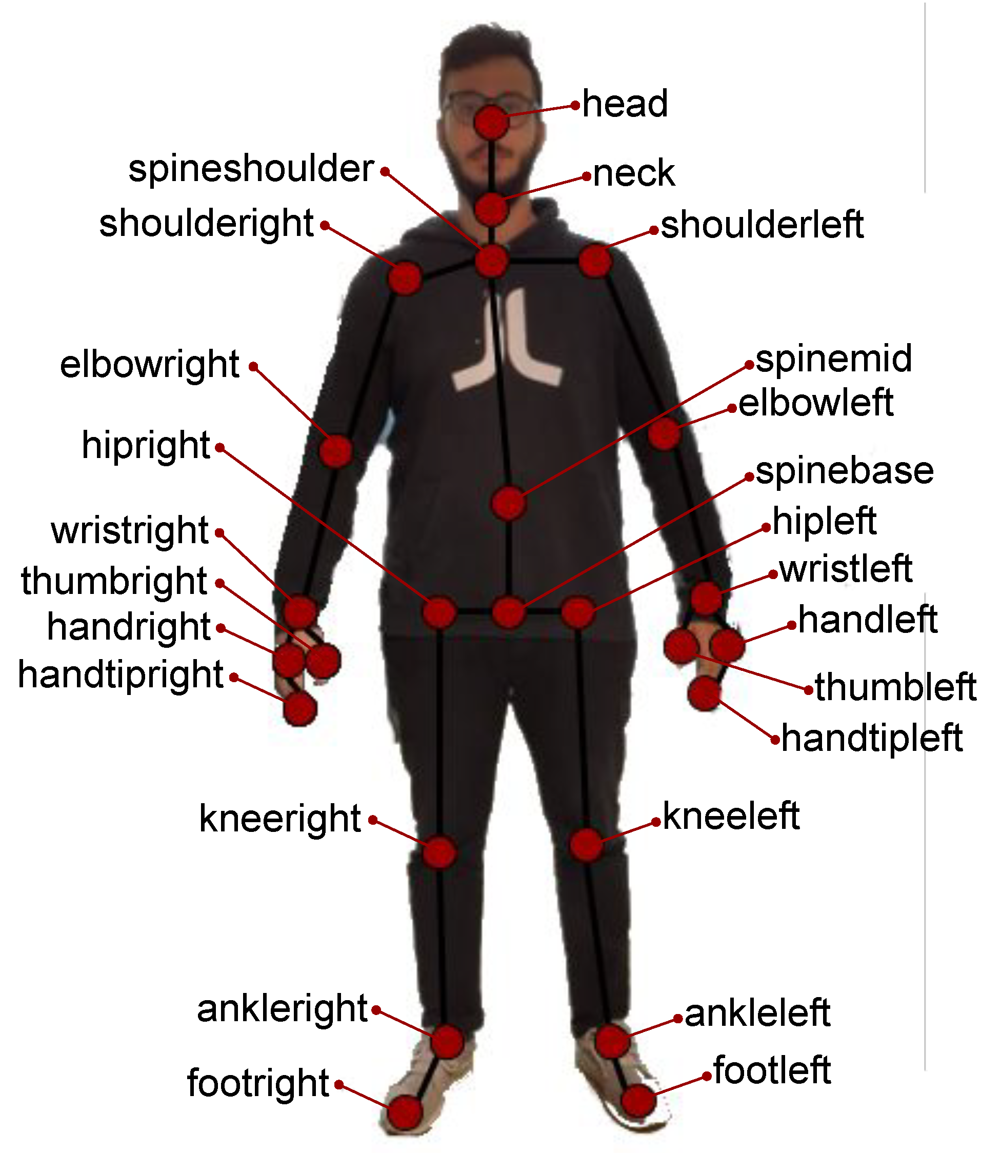
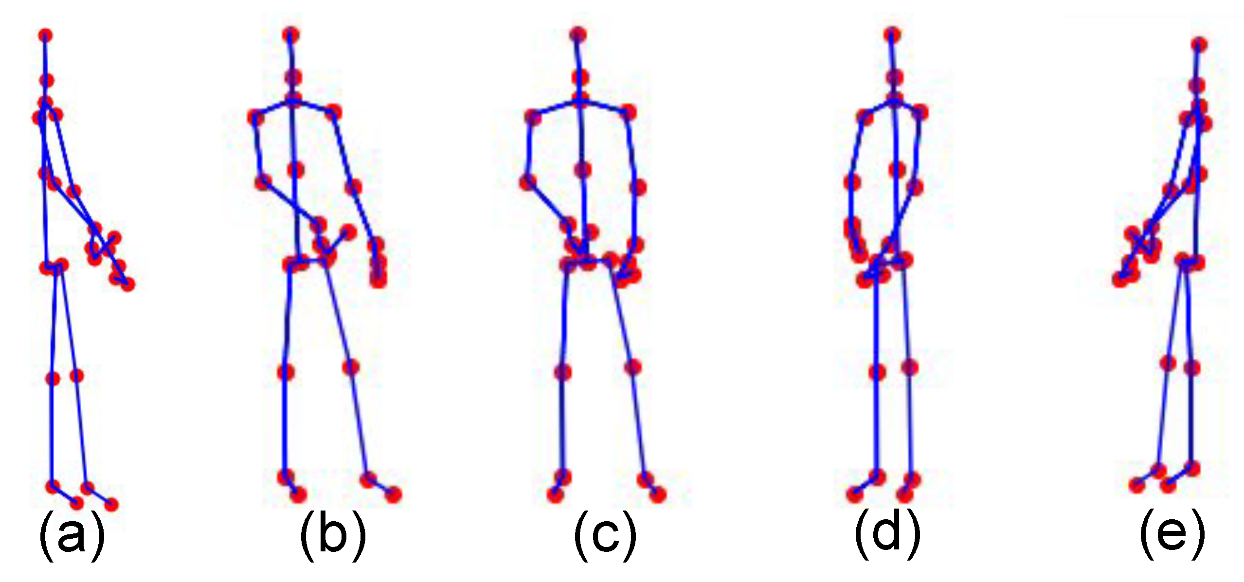
2.1. Human Activity Recognition

The approach we follow for human activity recognition has been presented in our previous work [26]. It is based on 3D skeletal motion information, resulting from video captured by an RGB and depth camera, namely the Microsoft Kinect v2 (https://developer.microsoft.com/en-us/windows/kinect). A set of 25 skeletal joints is extracted by the Kinect SDK and tracked in the 3D space and in real-time, while an actor performs a given activity. Interactions between actors are also being captured using a single camera, since Kinect supports simultaneous extraction of up to 6 skeletons. For each joint, its x, y and z coordinates are recorded. An example of an extracted skeleton is illustrated in Figure 1. Note that joints follow a graph-based representation; nodes correspond to joints, while edges connect neighboring joints.

Given the 3D skeletal information, we aim to provide a 2D image representation, so that it could be used with a typical CNN. The first step is to consider that a given joint’s motion within the 3D space consists of 3 1D signals, corresponding to the x, y and z coordinates over time. Upon concatenation of these signals, a 2D image is formed. Note that, though the number of rows of the aforementioned image is fixed for each activity and equal to 75, the number of columns may be different. This, due to the common fact that different actions could present significantly different temporal durations, for example, consider intuitively comparing the duration of activities such as “sitting down” and “wear jacket”. Obviously, the latter should require more time. Moreover, the same action, in the common case it is not performed by the actors, may require different temporal duration. Also, it should be intuitive that examples belonging to the same action, when performed repetitively by the same subject should have similar, yet unequal duration. This temporal variation is typically addressed by interpolation. Therefore, in our approach we impose a linear interpolation step. More specifically, we choose to se the duration of each action instance to $T_a=159$, so that the aforementioned image which we will refer to as “signal” image has a fixed size of $159\times 75$ for each activity. An example of a signal image that has been created with the aforementioned process is illustrated in Figure 2.

The next step is to create the image that will be fed to the CNN. This image will serve as an intermediate visual representation of the aforementioned skeletal sequences. A plethora of such representations has been proposed; all sharing the same motivation: to capture both spatial and temporal information regarding skeletal motion in the 3D space, over time. This information is reflected to the color and texture properties of the representation. Notable recent works include the one of Du et al. [28] who created chronologically arranged sequences of pseudocolored images, “joint trajectory maps” of Wang et al. [29] wherein texture corresponded to motion magnitude, “skeleton optical spectra” of Hou et al. [30], wherein hue changes corresponded to the temporal variation of motion, “joint distance maps” of Li et al. [31] who encoded joint distances and distance variations in a pair-wise sense, and finally of Ke et al. [32] who extracted invariant features by subsets of joints as in Reference [28] and upon processing, created a 2D representation.

In previous work [26] we have experimented with four of the most popular image transforms to the spectral domain, that is, Discrete Fourier Transform (DFT), Discrete Cosine Transform (DCT), Fast Fourier Transform (FFT) and Discrete Sine Transform (DST). Our examples showed that best accuracy was achieved using DST. Therefore, in this work we are limited to experiments using only DST, yet both data augmentation and domain adaptation, as will be presented in Section 2.2 and Section 2.3, respectively, may be applied to any 2D visual representation of 3D skeletal data. Therefore, DST is applied to each signal image, creating another 2D image which we will refer to as “activity image”. Upon applying DST we discard its phase, preserving only its magnitude. We further process this image by normalizing using the orthonorm. Finally, the result is a 2D image, corresponding to the signal spectrum of the signal image. An example signal image and the corresponding activity image are illustrated in Figure 2.

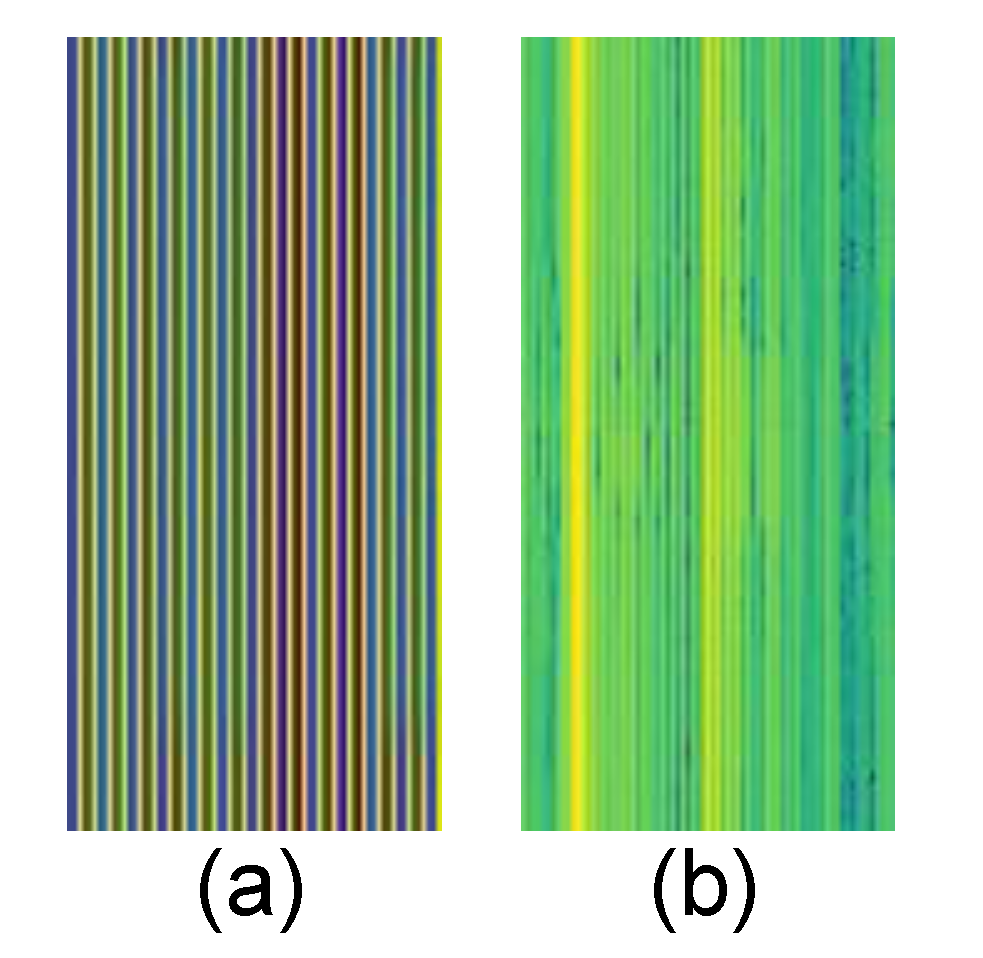
2.2. Data Augmentation

As we have already mentioned in Section 1, data augmentation aims to expand the size and/or the diversity of a given data set, by constructing some kind of synthetic images, by considering any properties/limitations of the problem at hand. In the context of HAR, data augmentation has been previously used with inertial measurements extracted from wearable sensors by Eyobu and Han [33], who applied local averaging as a down-sampling technique and shuffling. Also, using similar data, Kalouris et al. [34] applied a set of domain specific transformations, such as rotation, scaling, jittering and so forth. Hernandez et al. [35] worked with hand points and applied data warping on the magnitude and the temporal location of motion signals.

However, the aforementioned problem of viewpoint invariance has not been adequately addressed by intense research efforts. Liu et al. [36] proposed the direct application of geometric transformations to raw skeletal sequences. They created a 5D joint representation by concatenating 3D space coordinates, time and joint label. Then, in order to create a 2D image, they projected 2 of the aforementioned 5 dimensions, while the remaining 3 were mapped to R, G and B color values. Obviously, the resulting images were pseudo-colored. Moreover, we should emphasize that the proposed data augmentation approach has been partially inspired by the work of Zhang et al. [16]. Therein, a view adaptive RNN, was used in order to apply geometric transformations to raw skeletons captured under several views, towards the selection of more “consistent” viewpoints.

As it has already been mentioned, in this work we consider a multi-camera setup. We assume that each activity is captured by more than one cameras. Of course, in real-life scenarios, more than one cameras may be used for example, in an ADL cross-view recognition setup within an assistive living environment. When the camera setup is a priori known, we are able to align any camera to another by imposing a geometric transformation which may be decomposed to a set of rotations and translations, assuming that cameras are of the same type. In our case, the camera setup is known and consists of three cameras whose distance to the test subject is the same that is, placed at the perimeter of an imaginary circle. More specifically, one of the camera has been placed so as to directly face the test subject from the front. Also, the remaining two cameras have been placed at the left and the right of the test subject. Therefore, we are able to align any two given cameras by the simple rotation transformation [37], denoted by:

$${\mathbf{R}}_y\left(\theta \right)=\left[\begin{array}{ccc}cos\theta & 0& sin\theta \\ 0& 1& 0\\ -sin\theta & 0& cos\theta \end{array}\right].$$

(1)

For the examined case of data augmentation, our goal is to assist the training procedure of the CNN, by artificially increasing the number of training samples. Note that based on the way signal and activity images are created, traditional data augmentation strategies such as rotations and crops may not be applied, since these would severely affect the spectral properties of activity images. Instead, we choose to use activity samples of skeletal motion and process them so as to provide rotated instances taken by a given camera, in a way that they are aligned to another camera. Then, we construct signal and activity images, accordingly and preserve visual properties of activity images.

More specifically, the process of alignment of any two given skeletons that have been captured from different viewpoints is as follows—each 3D joint is rotated by an angle $\theta$, about the y-axis. This process complies to the Cartesian 3D coordinate system that has been adopted by Kinect v2, therefore is reflected to the actual action examples. The angle $\theta$ that is required by the rotation transformation is selected based on two factors: (a) the initial camera position setup; and (b) the pair of cameras that have been used for training and testing purposes. for example, let us consider two cameras, one placed at the subject’s left side and another placed at the subject’s right side. Let ${\theta }_L$ and ${\theta }_R$ denoting the aforementioned angles, respectively. In that case, the required transform that should be applied is ${\mathbf{R}}_y({\theta }_R-{\theta }_L)$ (see Equation (1)). An example of a raw skeleton that has been rotated by applying all angles that have been used throughout our study is illustrated in Figure 3.

2.3. Domain Adaptation

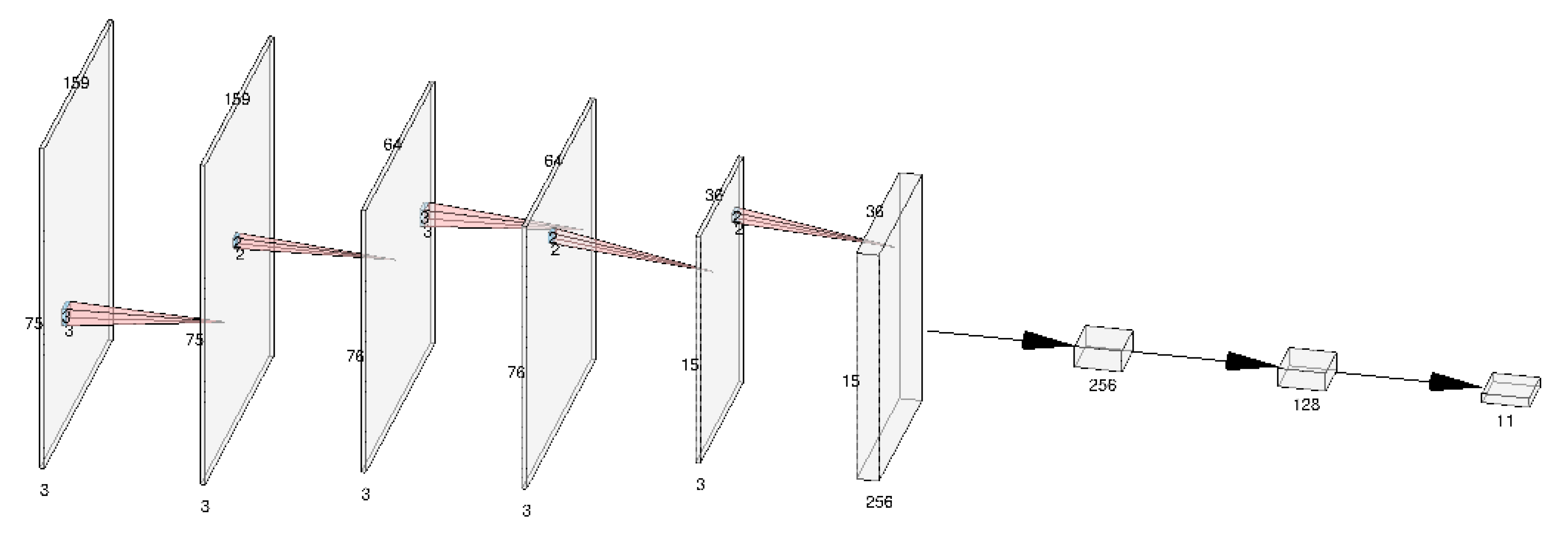
As discussed in the introduction, domain adaptation is a sub-field of transfer learning which aims to mitigate the covariate-shift problem when training a classifier. To make this more precise, consider, as is typical in domain adaptation literature [38], a classification problem as a tuple $(D,T)$, where D is called the domain and T the task. The domain is in turn a tuple $(\mathcal{X},P(X\left)\right)$, where $\mathcal{X}$ is the space in which the covariates take values and $P\left(X\right)$ is the marginal distribution of the covariates over $\mathcal{X}$. The task is another tuple $(\mathcal{Y},P(Y\left|X\right))$, where $\mathcal{Y}$ is the label space and $P\left(Y\right|X)$ is the conditional distribution of labels given values of the covariates. In standard supervised learning we are typically interested in approximating $Pr\left(Y\right|X)$, that is, obtain a predictor for T. In domain adaptation, the setup usually consists of two problems $(D_s,T_s)$, $(D_t,T_t)$, respectively called the source and target problems, such that $T_s=T_t$ but $D_s\ne D_t$. In this work we focus on homogeneous domain adaptation where we further assume that ${\mathcal{X}}_s={\mathcal{X}}_t$, but $P\left(X_s\right)\ne P\left(X_t\right)$.

The domain adaptation problem is to utilize $(D_s,T_s)$ or a predictor for $T_s$ so as to obtain a predictor for $T_t$ or improve a predictor for $T_t$. This is particularly useful to consider in a transductive learning scenario where the (unlabeled or sparsely labeled) test set is available during training. In general two general approaches are followed; the first involves importance sampling techniques, while the second involves learning a representation for source and target data in which the covariate-shift problem is resolved, that is, where the distribution of source and target data is the same [38]. Deep learning algorithms for obtaining such representations have been widely explored yielding many successful methods [39], especially in the field of computer vision [38]. In particular, adversarial neural networks have proven to be an effective tool for mitigating the covariate-shift problem and have been successfully employed in multiple works [10,11,40]. Such methods, are flexible and well suited for the domain adaptation task because they allow for the automatic extraction of representations, where the distributions of source and target data are the same, using simple iterative optimization algorithms. In this work we focus on adversarial domain adaptation techniques for our evaluation of domain adaptation in computer vision tasks.

Adversarial domain adaptation schemes were inspired by the distribution alignment approach presented in Reference [41], within the context of generative adversarial networks. A general abstract scheme that breaks down such methods is presented in Reference [10]. Typically, two representation extracting networks $M_s,M_t$ are defined, along with a domain discriminator network D and a source classifier C which discriminates source data instances based on the representation extracted from $M_s$. The source networks $M_s$ and C are either jointly trained on source data before the adaptation procedure or trained along with the $M_t$ and D during adaptation in an alternating manner. In practice, the former approach is more susceptible to poor local minima for example, mode collapse, while the second approach is very unstable during training and difficult to converge. For a contrast of the two approaches see for example, References [10,11] respectively. Experimentally, we found the former approach to be more practical, with better results in our task.

As such, the training procedure as adopted in the experimental section in this work takes the following form. Firstly, the source networks are trained in a standard supervised learning manner over the source data using the categorical cross-entropy loss function. The weight of $M_s,C$ are then fixed. In turn, we initialize the target representation network $M_t$ with the weights of $M_s$. This is a standard step in adversarial domain adaptation literature which helps avoid poor local minima [10]. The domain discriminator is initialized randomly and must be chosen with more parameters than the classifier network C in accordance with Reference [42] and the principle that for effective domain adaptation and a particular representation, it should be harder to discriminate domains than discriminating classes. At each step during training, a batch of source and target instances is sampled and the corresponding representations are computed using $M_s$ and $M_t$. The domain discriminator is the trained in a standard supervised manner to discriminate between instances from source and target domain. Once D is updated, its weights are fixed, and the target representation network $M_t$ is trained in a similar manner but using the reversed D gradients.

This process can be shown to minimize the Jensen-Shannon divergence [43] between the distribution of source and target instances in latent space, that is, the distributions of the outputs of $M_s$ and $M_t$, if at each step the discriminator D is trained to optimality. For this reason, it is a good practice to perform multiple updates on the parameters of D for each update of parameters of $M_t$. However care must be taken since if D can perfectly discriminate between the two domains, there is no gradient feedback to continue training [44]. For this reason one needs to carefully adjust the number of iterations for D before each update of $M_t$. After convergence, the source classifier network C can be used to classify target images mapped into the latent space by $M_t$. This is because the covariate shift problem has been mitigated in the latent space, and by assumption $T_s=T_t$ and hence $P\left(Y\right|X)$, which C approximates, is the same for both domains. Note that alternative schemes have been formulated which lead, for example, in minimizing the Wasserstein-1 distance between the two distributions, in the context of GANs.

The method described above can be utilized without access to any target data labels. However, having such labeled target data can help improve the performance of the target classifier as it may help guide the adaptation procedure and aid in avoiding poor local minima. In particular, a method for incorporating target label knowledge into standard adversarial domain adaptation schemes is explored in Reference [40]. Essentially, the loss function for training $M_t$ combines a standard supervised learning term and a domain confusion term. For the former the network $C\circ M_t$ is trained with the parameters of C kept constant, while for the latter a similar procedure as the one described above is employed.

The described approach, formulated in further detail in Reference [40], needs careful hyper-parameter tuning. In particular, the design choices including standard network topology, batch size, learning rates e.t.c., require careful tuning because training occurs as an interplay between multiple networks whose training capacity affects the training of the other networks. In addition, one needs to tune the tradeoff parameter between the domain confusion term and the supervision signal term in the objective function. Large values of the parameter may lead to overfitting while lower values may hinder training. In addition, as mentioned above, it is important to tune the number of training iterations of the domain discriminator network per training iteration of the target representation network. Typically, grid search should be applied but we note that tuning these parameters may introduce a substantial computational overhead.

2.4. Classification

In this section we present the deployed CNN architecture used throughout the experimental section of this work (Figure 4). In brief, three convolutional layers are used to obtain high-level features, followed by two fully connected layers performing the classification. Max-pooling layers are used to sub-sample each convolution result. To help improve the generalization capabilities of our model, in this work we follow a popular approach and apply the dropout regularization technique [45], in which at each training stage several nodes are “dropped out” of the network. This helps to avoid complex co-adaptations between neurons which lead to overfitting. In addition, we use a validation set to monitor the validation loss and we utilize the early stopping technique. In more detail, the first convolutional layer filters the 159 × 75 input activity image with 32 kernels of size 3 × 3, the second convolution uses 64 kernels of size 3 × 3 over the input 76 × 34 image and the third convolutional layer filters the 36 × 15 resulting image with 128 kernels of size 3 × 3. At each stage, 2 × 2 “max-pooling” is applied. The aforementioned architecture has been selected through validation set tuning based on two factors: (a) the need to build sufficiently rich representations to allow for effective classification; and (b) the restriction of the number of parameters so as to allow flexibility, for example, for easy deployment of the model in low-cost platforms or mobile devices to perform inference on the edge, in real-life applications of the herein proposed approaches.

3. Experiments

In this section, firstly we present the dataset that we have chosen for the experimental evaluation of the proposed approach. Then, we present the evaluation protocols that we have followed for the data augmentation and the domain adaptation approach, followed by the presentation and the discussion of the corresponding results and comparisons with baseline approaches. Finally, we present the implementation details regarding hardware and software used.

3.1. Dataset

For the experimental evaluation of our approach we used the PKU-MMD dataset [20]. PKU-MMD consists a large-scale benchmark dataset that focuses on human action understanding. It contains approx. 20 K action instances from 51 action categories, spanning into 5.4 M video frames and performed by 66 human subjects. A multi-camera setup was used throughout the recording sessions. More specifically, data from 3 Microsoft Kinect v2 cameras have been collected. For each action instance, PKU-MMD provides the four following modalities: (a) raw RGB video sequences, each depicting one or more actors while performing an action/interaction under a given viewpoint; (b) depth sequences, that is, the z-dimension corresponding to the scene depth at each pixel of an RGB sequence; (c) infrared radiation sequences, that is, modulated infrared light captured simultaneously to the RGB sequences; and (d) positions in the 3D space of the extracted human skeleton joints, varying over time. Recordings from 3 camera views are available; each action is simultaneously captured by all cameras. Note that the users were asked to perform the actions within a pre-determined area of 180 cm length and 120 cm width, so as their distance to the cameras would remain as fixed as possible. Also, they were asked to face towards one of the cameras (not necessarily the middle one). At the following, we shall use the following naming convention for the three camera views: L (left), M (middle) and R (right). As illustrated in Figure 5, the 3 cameras are placed at the perimeter of an imaginary circle, while the following fixed angles are used for their positioning: $-{45}^{\circ }$, $0^{\circ }$ and $+{45}^{\circ }$. Also, the cameras have been placed on the same height level, which also remains fixed and equal to 120 cm for all activities. Also, since videos contain several sequential actions, inter-video temporal boundaries are available.

As we have already mentioned, our study aims to assess whether and how the proposed data augmentation strategies may be used to assist human activity recognition. Our use case is an ambient assistive living scenario, where the goal is the recognition of ADLs. Therefore, we selected 11 out of the 51 classes of PKU-MMD, which we believe are the most close to ADLs or events in such a scenario. The selected classes are: eat meal snack, falling, handshaking, hugging other person, make a phone call answer phone, playing with phone tablet, reading, sitting down, standing up, typing on a keyboard and wear jacket. Note that we worked only using the skeletal data, that is, we discarded RGB, depth and infrared information. Indicative activity images for the 11 classes that will be used throughout our experimental evaluation are illustrated in Figure 6.

3.2. Implementation Details

All experiments that will be presented in this section have been performed using a personal workstation running Ubuntu 18.04 (64 bit) with the following specifications: Intel™i7 5820K 12 core processor @ 3.30 GHz, equipped with 16 GB RAM and an NVIDIA™Geforce GTX 2060 GPU with 8 GB RAM. The deep CNN architecture has been implemented in Python, using Keras 2.2.4 [46] with the Tensorflow 1.12 [47] backend. All data pre-processing and processing steps have been implemented in Python 3.6 using NumPy (http://www.numpy.org/), SciPy (https://www.scipy.org/) and OpenCV (https://opencv.org/).

3.3. Evaluation and Results

Typical evaluation protocols followed in similar research works, benefit from datasets such as the aforementioned one [20], providing several types of benchmarks. The most obvious one is to conduct experiments per camera position (single view). In this case, both training and testing sets derive from the same viewpoint for example, samples from L camera view are used both for training and testing. The second case requires different camera viewpoints for training and testing. Note that more than one camera viewpoints may be used for training or testing, for example, samples from L camera view are used for training while samples from R camera view are used for testing. The goal of such experiments is to test the robustness of a given approach in terms of typical geometric transformations (i.e., a rotation). This may be regarded as a simulation of a real-life case of abrupt viewpoint changes, typically occurring when subjects are not limited to a relatively small area or are not required to face directly a given camera. In real-life situations this is expected to happen when a system is trained for example, within a laboratory environment and is deployed into a real-life environment. Therefore, in this work we are limited to experiments where training and testing sets derive from different viewpoints.

3.3.1. Data Augmentation

The evaluation protocol we have used for the case of augmentation is as follows: based on the camera setting of the PKU-MMD data, and the coordinate system used by the Microsoft Kinect v2 camera, we applied rotation transformations on signal images (to be more specific, on the x, y and z coordinates of skeleton data), as discussed in Section 2.2. More specifically, we performed rotations using $\theta \in \{\pm {45}^{\circ },\pm {90}^{\circ }\}$. We should herein highlight that L signal images, when rotations of $-{45}^{\circ }$ and $-{90}^{\circ }$ are applied, align to M, R, respectively. Similarly M signal images when rotations of ${45}^{\circ }$ and $-{45}^{\circ }$ are applied align to L, R, respectively, while R signal images when rotations of ${45}^{\circ }$, ${90}^{\circ }$ are applied align to M, L, respectively. Obviously, the aforementioned process results to a multiplication of the number of available images by a factor of 5. We may now use this augmented data set instead of the original one for training, aiming to achieve a significant increase in the classification performance of our model. In other words, our goal could be alternatively stated as follows: under a given camera viewpoint, provide more reliable recognition of human actions upon training with an augmented data set; the latter comprises of all aligned images that resulted from the aforementioned rotation transformations. Experimental results of data augmentation are presented in

Table 1. Experimental results. Figures represent average accuracy percentages over ten runs. In each setup best accuracy achieved is indicated with bold. For each viewpoint adaptation scenario, for example, “Left to Middle” (indicated $L\to M$) the four numbers (0, 1, 5 and 10) indicate the percentage of target data instances which are labelled. S is the source model, built by a simple cross-view experiment. $T_{rand}$ and $T_{w_S}$ denote models whose initial weights have been taken randomly and from S, respectively. Note that with no labeled data in the target domain (i.e., 0) these models cannot be trained and hence these columns are omitted.

	Baselines									Data Augmentation	Domain Adaptation
	S	${\mathit{T}}_{{\mathit{w}}_{\mathit{S}}}$				${\mathit{T}}_{\mathit{rand}}$					0	1	5	10
		0	1	5	10	0	1	5	10
$L\to M$	0.85	-	0.85	0.86	0.92	-	0.61	0.73	0.77	0.93	0.84	0.86	0.89	0.92
$L\to R$	0.41	-	0.60	0.70	0.75	-	0.51	0.61	0.71	0.85	0.50	0.63	0.78	0.82
$M\to L$	0.83	-	0.83	0.87	0.90	-	0.51	0.68	0.79	0.85	0.83	0.84	0.87	0.91
$M\to R$	0.78	-	0.80	0.85	0.90	-	0.51	0.70	0.76	0.90	0.83	0.83	0.86	0.91
$R\to L$	0.44	-	0.60	0.76	0.81	-	0.51	0.65	0.77	0.69	0.53	0.65	0.80	0.86
$R\to M$	0.85	-	0.85	0.86	0.91	-	0.61	0.70	0.77	0.88	0.85	0.85	0.88	0.92
mean	0.69	-	0.76	0.82	0.87	-	0.54	0.68	0.76	0.85	0.73	0.78	0.85	0.89

and

Table 2. Experimental results. Figures represent average F1 scores over ten runs. In each setup best F1 score achieved is indicated with bold. As in Table 1, for each viewpoint adaptation scenario, for example, “Left to Middle” (indicated $L\to M$) the four numbers (0, 1, 5 and 10) indicate the percentage of target data instances which are labelled. S is the source model, built by a simple cross-view experiment. $T_{rand}$ and $T_{w_S}$ denote models whose initial weights have been taken randomly and from S, respectively. Note that with no labeled data in the target domain (i.e., 0) these models cannot be trained and hence these columns are omitted.

	Baselines									Data Augmentation	Domain Adaptation
	S	${\mathit{T}}_{{\mathit{w}}_{\mathit{S}}}$				${\mathit{T}}_{\mathit{rand}}$					0	1	5	10
		0	1	5	10	0	1	5	10
$L\to M$	0.85	-	0.90	0.90	0.85	-	0.61	0.71	0.78	0.92	0.81	0.77	0.86	0.88
$L\to R$	0.42	-	0.67	0.81	0.82	-	0.49	0.53	0.57	0.82	0.51	0.55	0.727	0.79
$M\to L$	0.84	-	0.81	0.88	0.93	-	0.48	0.57	0.64	0.83	0.81	0.86	0.85	0.94
$M\to R$	0.79	-	0.80	0.83	0.90	-	0.47	0.65	0.71	0.90	0.80	0.81	0.83	0.92
$R\to L$	0.45	-	0.78	0.77	0.82	-	0.47	0.53	0.57	0.65	0.52	0.67	0.80	0.88
$R\to M$	0.86	-	0.84	0.88	0.92	-	0.55	0.64	0.77	0.86	0.86	0.71	0.86	0.88
mean	0.71	-	0.80	0.85	0.87	-	0.51	0.59	0.67	0.83	0.72	0.73	0.83	0.88

.

3.3.2. Domain Adaptation

Moreover, the evaluation protocol we have used for the case of domain adaptation is as follows: one of the camera views is selected as source data, while another on as target data. At the following, we shall use the typical notation $X\to Y$, which denotes adaptation between source X and target Y. For the sake of the presentation, the same notation shall be used also in the augmentation case, denoting training set X and testing set Y. Therefore, we evaluate our approach for all possible combinations, that is, $L\to R,L\to M,R\to M,R\to L,M\to L$ and $M\to R$. Also, considering the semi-supervised setting that we have presented in Section 2.3, in this case it is required to use a small, labeled subset of the target data; these examples serve as labeled target instances and are utilized during training both for providing a supervision signal and for unsupervised adversarial training. Of course, this subset is excluded when calculating validation accuracy both in this case and also in the case of augmentation. In every combination, the percentage of the labeled target data varies between $0\%,1\%,5\%$ and $10\%$, while a source model $\left(S\right)$ is trained in a standard supervised way on the source domain. Experimental results of domain adaptation are presented in Table 1 and Table 2.

3.3.3. Comparisons to Other Approaches

We should herein note that to the best of our knowledge, our approach is the first that (a) applies data augmentation in raw skeletal data; and (b) applies an adversarial domain adaptation strategy. Therefore, in order to compare the aforementioned strategies, we used the following baselines: (a) the standard (source) model S; (b) a model with random initial weights, that is, $T_{rand}$; and (c) a model with initial weights taken from S, that is, $T_{w_S}$. This last approach represents a widely utilized class of transfer learning techniques known as fine tuning methods [38]. Results of baseline approaches are presented in Table 1 and Table 2.

3.4. Discussion

The results of this study have indicated that both of the reviewed techniques offer substantial improvement to the generalization capabilities of HAR classifiers in the cross-view scenario. In particular, comparing these methods with $T_{rand}$ model results, which corresponds to vanilla supervised learning without any cross domain knowledge transfer and when labelled data are scarce, we observe a significant performance boosts. Moreover, the source domain S often outperforms the $T_{rand}$ model (when the viewpoint change is mild, for example, $L\to M$) highlighting the potential benefit of cross-domain data when training viewpoint robust classifiers. The benefit of utilizing data augmentation and domain adaptation is made much more apparent in more extended viewpoint changes (e.g., $L\to R$ as opposed to $L\to M$), where simply using a source model trained on a viewpoint different than the test set gives poor performance.

We further observe that data augmentation typically performs much better than domain adaptation when no target labels are available. In particular, the accuracy of models trained with data augmentation techniques are much less dependent on the underlying cross-view adaptation than the corresponding domain adaptation results. Domain adaptation yields almost no improvement for easy viewpoint changes while it yields satisfying improvement for harder viewpoint changes, albeit much less significant than the ones achieved through augmentation. In the semi-supervised setting the domain adaptation approach substantially benefits from the presence of a supervision signal which guides the adaptation process. The performance of adapted models in this setting is much more consistent between different cross-view adaptation instances and on average outperforms the plain data augmentation approach.

Although in the semi-supervised setting domain adaptation provides the best accuracy out of the examined methods, the associated hyper-parameter tuning may become an important issue when deploying such methods for real-life applications, generating a substantial computational overhead. In particular, we observed significant sensitivity to learning rates, the trade-off parameter between the domain confusion and the supervision signal term in the adversarial objective function and the number of updates on the domain discriminator weights per update of the target representation network updates. On the other hand, producing synthetic data to capture the effect of changing the viewpoint is relatively cheap and may be preferred for many practical HAR tasks. Moreover, the percentage of labeled data played a crucial role in domain adaptation results. In cases where target domain labelled data is less abundant, an augmentation approach for cross view activity recognition is observed to be a more appropriate choice altogether.

4. Conclusions and Future Work

In this work we addressed the problem of lack of a sufficient amount of labeled data that are necessary when training a model that would be used for human activity recognition. In particular, in many real-life applications, the data collection and annotation process may be a very costly and/or slow process. To overcome this limitation, two popular approaches are (a) data augmentation, that is, techniques aiming to the creation of synthetic data for the expansion of the size and/or the diversity of the data set; and (b) domain adaptation, that is, techniques aiming to mitigate the covariate shift problem given that training and evaluation sets derive from the same distribution. Herein, we experimented with a viewpoint data augmentation approach, aiming to allow models to demonstrate increased accuracy when viewpoint in evaluation data is different than the one in the available training data. We also experimented with an adversarial domain adaptation approach, under the assumption that part of the testing data were labeled and excluded from evaluation.

Our study was based on previous work regarding classification of human activity in videos, based on 3D skeletal motion data. We used a 2D image representation of these data, which relies on spectral images that have been obtained through the application of DST on raw data. Note that both data augmentation and domain adaptation approaches that we propose are agnostic to the way this representation is formed. Since the experimental setup comprised of three cameras, that is, three different viewpoints our goal was to transfer knowledge from one viewpoint to another. In other words, we have trained a model using samples captured under a single viewpoint (source model). Evaluation used only samples from a different viewpoint. Since the angle is significantly different, a drop of performance is expected, making them impractical for real-life applications. However, the application of both transfer approaches enabled a significant increase of performance in this cross-view scenario. We evaluated the proposed approach using a popular action recognition dataset as a source, focusing on a subset of 11 actions which we believe are the most close to real-life ADLs.

Our experiments showed that when target data are fully unlabelled, data augmentation offers a huge increase over the source model. However, a small amount of labeled data makes domain adaptation approach to exhibit clearly improved performance overall, making it practical for real-life applications. For example, consider an assistive living scenario, where a single camera is used to monitor the behaviour of a human subject. Typically, in such scenarios the space where subjects act are not strictly limited. Therefore, the viewpoint may significantly change. Now, consider an activity recognition model that has been pre-trained in laboratory conditions. In case that the subject is able to participate in a data collection process, it should be more effective to adopt a domain adaptation approach. Of course, if this is not possible, then data augmentation is able to offer an adequate alternative, while it is able to be immediately applied.

Regarding the limitations of the proposed approach, we should note the following: Firstly, since it is based on skeleton data, those should be available, either using some specific hardware such as the Microsoft Kinect and its API, or some skeleton extraction library such as OpenPose [48]. Although the latter may be used without some specialised video capturing hardware, it is by far more computationally expensive; its use for real-time applications may be impractical without using a modern GPU. Of course, reliable skeleton extraction is prone to illumination/viewpoint changes and occlusion. Next steps, that is, creation of signal and activity images are “instant”. Regarding model training and for the deep architecture that has been described in Section 2.4, training using the configuration described in Section 3.2 typically requires less than an hour, while the trained model requires 1.2 msec using a GPU and 8.3 msec without using a GPU for classification of an action sample. In implementing data augmentation, the number of training samples is increased by a factor of 5, which in turn may increase training times by approx. a factor of 2. On the other hand, the domain adaptation approach that has been adopted in the context of this work introduces a significant training overhead. Firstly, the adversarial training process consumes a lot of memory compared to standard supervised learning and if this cannot be covered by the underlying computation unit (e.g., GPU, CPU/RAM) training time may significantly increase as hard disk swap is utilized. Moreover, the training process is prone to instability and for this reason small learning rates and many iterations are required for convergence. We should emphasize that in real-life applications, a segmentation step should be imposed before the creation of activity images causing a further delay. Finally, we should note that as far as this work is concerned, both data augmentation and domain adaptation approaches are agnostic to the limitations of video/skeleton capturing and of the formulation of activity images.

In the future, we plan to apply the proposed approach on methods for creating the signal image, possibly with the use of other types of sensor measurements such as wearable accelerometers, gyroscopes and so on and investigate on image processing methods for transforming the signal image to the activity image. Furthermore, we will exploit other types of visual modalities in the process, such as RGB and depth data and we will evaluate our proposed approach on several public datasets. In addition, we are currently investigating procedures for combining data augmentation and domain adaptation techniques. Finally, we will apply our techniques in a real-life assistive living environment and we our willing to extend our approach to open set domain adaptation for applications where the target dataset contains previously unseen (in the source domain) classes.

References

1. Sun, C.; Shrivastava, A.; Singh, S.; Gupta, A. Revisiting unreasonable effectiveness of data in deep learning era. In Proceedings of the IEEE International Conference on Computer Vision, Venice, Italy, 22–29 October 2017; pp. 843–852. [Google Scholar]
2. Shorten, C.; Khoshgoftaar, T.M. A survey on image data augmentation for deep learning. J. Big Data 2019, 6, 60. [Google Scholar] [CrossRef]
3. Van Dyk, D.A.; Meng, X.L. The art of data augmentation. J. Comput. Graph. Stat. 2001, 10, 1–50. [Google Scholar] [CrossRef]
4. Ding, J.; Chen, B.; Liu, H.; Huang, M. Convolutional neural network with data augmentation for SAR target recognition. IEEE Geosci. Remote Sens. Lett. 2016, 13, 364–368. [Google Scholar] [CrossRef]
5. Li, B.; Dai, Y.; Cheng, X.; Chen, H.; Lin, Y.; He, M. Skeleton based action recognition using translation-scale invariant image mapping and multi-scale deep CNN. In Proceedings of the 2017 IEEE International Conference on Multimedia & Expo Workshops (ICMEW), Hong Kong, China, 10–14 July 2017; pp. 601–604. [Google Scholar]
6. Ben-David, S.; Blitzer, J.; Crammer, K.; Kulesza, A.; Pereira, F.; Vaughan, J.W. A theory of learning from different domains. Mach. Learn. 2010, 79, 151–175. [Google Scholar] [CrossRef] [Green Version]
7. Patel, V.M.; Gopalan, R.; Li, R.; Chellappa, R. Visual domain adaptation: A survey of recent advances. IEEE Signal Process. Mag. 2015, 32, 53–69. [Google Scholar] [CrossRef]
8. Redko, I.; Morvant, E.; Habrard, A.; Sebban, M.; Bennani, Y. Advances in Domain Adaptation Theory; Elsevier: Amsterdam, The Netherlands, 2019. [Google Scholar]
9. Zhang, J.; Han, Y.; Tang, J.; Hu, Q.; Jiang, J. Semi-supervised image-to-video adaptation for video action recognition. IEEE Trans. Cybern. 2016, 47, 960–973. [Google Scholar] [CrossRef]
10. Tzeng, E.; Hoffman, J.; Saenko, K.; Darrell, T. Adversarial discriminative domain adaptation. In Proceedings of the IEEE Conference on Computer Vision and Pattern Recognition, Honolulu, HI, USA, 21–26 July 2017; pp. 7167–7176. [Google Scholar]
11. Ajakan, H.; Germain, P.; Larochelle, H.; Laviolette, F.; Marchand, M. Domain-adversarial neural networks. arXiv 2014, arXiv:1412.4446. [Google Scholar]
12. Cao, Z.; Long, M.; Wang, J.; Jordan, M.I. Partial transfer learning with selective adversarial networks. In Proceedings of the IEEE Conference on Computer Vision and Pattern Recognition, Salt Lake City, UT, USA, 18–22 June 2018; pp. 2724–2732. [Google Scholar]
13. Cao, Z.; Ma, L.; Long, M.; Wang, J. Partial adversarial domain adaptation. In Proceedings of the European Conference on Computer Vision (ECCV), Munich, Germany, 8–14 September 2018; pp. 135–150. [Google Scholar]
14. Cao, Z.; You, K.; Long, M.; Wang, J.; Yang, Q. Learning to transfer examples for partial domain adaptation. In Proceedings of the IEEE Conference on Computer Vision and Pattern Recognition, Long Beach, CA, USA, 15–20 June 2019; pp. 2985–2994. [Google Scholar]
15. Hu, J.; Tuo, H.; Wang, C.; Qiao, L.; Zhong, H.; Jing, Z. Multi-Weight Partial Domain Adaptation. In Proceedings of the BMVC, Cardiff, UK, 9–12 September 2019; p. 5. [Google Scholar]
16. Zhang, P.; Lan, C.; Xing, J.; Zeng, W.; Xue, J.; Zheng, N. View adaptive recurrent neural networks for high performance human action recognition from skeleton data. In Proceedings of the IEEE International Conference on Computer Vision, Venice, Italy, 22–29 October 2017; pp. 2117–2126. [Google Scholar]
17. Aggarwal, J.K. Human activity recognition-A grand challenge. In Proceedings of the Digital Image Computing: Techniques and Applications (DICTA’05), Cairns, Australia, 6–8 December 2005; p. 1. [Google Scholar]
18. Wang, P.; Li, W.; Ogunbona, P.; Wan, J.; Escalera, S. RGB-D-based human motion recognition with deep learning: A survey. Comput. Vis. Image Underst. 2018, 171, 118–139. [Google Scholar] [CrossRef] [Green Version]
19. Liu, J.; Shahroudy, A.; Perez, M.L.; Wang, G.; Duan, L.Y.; Chichung, A.K. Ntu rgb+ d 120: A large-scale benchmark for 3d human activity understanding. IEEE Trans. Pattern Anal. Mach. Intell. 2019. [Google Scholar] [CrossRef] [Green Version]
20. Liu, C.; Hu, Y.; Li, Y.; Song, S.; Liu, J. Pku-mmd: A large scale benchmark for continuous multi-modal human action understanding. arXiv 2017, arXiv:1703.07475. [Google Scholar]
21. Paraskevopoulos, G.; Spyrou, E.; Sgouropoulos, D.; Giannakopoulos, T.; Mylonas, P. Real-time arm gesture recognition using 3D skeleton joint data. Algorithms 2019, 12, 108. [Google Scholar] [CrossRef] [Green Version]
22. Schuldt, C.; Laptev, I.; Caputo, B. Recognizing human actions: a local SVM approach. In Proceedings of the 17th International Conference on Pattern Recognition, ICPR 2004, Cambridge, UK, 23–26 August 2004; Volume 3, pp. 32–36. [Google Scholar]
23. LeCun, Y.; Bottou, L.; Bengio, Y.; Haffner, P. Gradient-based learning applied to document recognition. Proc. IEEE 1998, 86, 2278–2324. [Google Scholar] [CrossRef] [Green Version]
24. Graves, A.; Mohamed, A.R.; Hinton, G. Speech recognition with deep recurrent neural networks. In Proceedings of the 2013 IEEE International Conference on Acoustics, Speech and Signal Processing, Vancouver, Canada, 26–31 May 2013; pp. 6645–6649. [Google Scholar]
25. Shotton, J.; Fitzgibbon, A.; Cook, M.; Sharp, T.; Finocchio, M.; Moore, R.; Kipman, A.; Blake, A. Real-time human pose recognition in parts from single depth images. In Proceedings of the CVPR 2011, Colorado Springs, CO, USA, 20–25 June 2011; pp. 1297–1304. [Google Scholar]
26. Papadakis, A.; Mathe, E.; Vernikos, I.; Maniatis, A.; Spyrou, E.; Mylonas, P. Recognizing human actions using 3d skeletal information and cnns. In Proceedings of the International Conference on Engineering Applications of Neural Networks, Crete, Greece, 24–26 May 2019; Springer: Cham, Switzerland, 2019; pp. 511–521. [Google Scholar]
27. Lawton, M.P.; Brody, E.M. Assessment of older people: self-maintaining and instrumental activities of daily living. Gerontologist 1969, 9, 179–186. [Google Scholar] [CrossRef] [PubMed]
28. Du, Y.; Fu, Y.; Wang, L. Skeleton based action recognition with convolutional neural network. In Proceedings of the 2015 3rd IAPR Asian Conference on Pattern Recognition (ACPR), Kuala Lumpur, Malaysia, 3–6 November 2015; pp. 579–583. [Google Scholar]
29. Wang, P.; Li, W.; Li, C.; Hou, Y. Action recognition based on joint trajectory maps with convolutional neural networks. Knowl. Based Syst. 2018, 158, 43–53. [Google Scholar] [CrossRef] [Green Version]
30. Hou, Y.; Li, Z.; Wang, P.; Li, W. Skeleton optical spectra-based action recognition using convolutional neural networks. IEEE Trans. Circuits Syst. Video Technol. 2018, 28, 807–811. [Google Scholar] [CrossRef]
31. Li, C.; Hou, Y.; Wang, P.; Li, W. Joint distance maps based action recognition with convolutional neural networks. IEEE Signal Process. Lett. 2017, 24, 624–628. [Google Scholar] [CrossRef] [Green Version]
32. Ke, Q.; An, S.; Bennamoun, M.; Sohel, F.; Boussaid, F. Skeletonnet: Mining deep part features for 3-d action recognition. IEEE Signal Process. Lett. 2017, 24, 731–735. [Google Scholar] [CrossRef] [Green Version]
33. Steven Eyobu, O.; Han, D.S. Feature representation and data augmentation for human activity classification based on wearable IMU sensor data using a deep LSTM neural network. Sensors 2018, 18, 2892. [Google Scholar] [CrossRef] [Green Version]
34. Kalouris, G.; Zacharaki, E.I.; Megalooikonomou, V. Improving CNN-based activity recognition by data augmentation and transfer learning. In Proceedings of the 2019 IEEE 17th International Conference on Industrial Informatics (INDIN), Helsinki-Espoo, Finland, 22–25 July 2019; Volume 1, pp. 1387–1394. [Google Scholar]
35. Hernandez, V.; Suzuki, T.; Venture, G. Convolutional and recurrent neural network for human activity recognition: Application on American sign language. PLoS ONE 2020, 15, e0228869. [Google Scholar] [CrossRef] [Green Version]
36. Liu, M.; Liu, H.; Chen, C. Enhanced skeleton visualization for view invariant human action recognition. Pattern Recognit. 2017, 68, 346–362. [Google Scholar] [CrossRef]
37. Theoharis, T.; Papaioannou, G.; Platis, N.; Patrikalakis, N.M. Graphics and Visualization: Principles & Algorithms; CRC Press: Boca Raton, FL, USA, 2008. [Google Scholar]
38. Csurka, G. A comprehensive survey on domain adaptation for visual applications. In Domain Adaptation in Computer Vision Applications; Springer: Cham, Switzerland, 2017; pp. 1–35. [Google Scholar]
39. Wang, M.; Deng, W. Deep visual domain adaptation: A survey. Neurocomputing 2018, 312, 135–153. [Google Scholar] [CrossRef] [Green Version]
40. Pikramenos, G.; Mathe, E.; Vali, E.; Vernikos, I.; Papadakis, A.; Spyrou, E.; Mylonas, P. An adversarial semi-supervised approach for action recognition from pose information. Neural Comput. Appl. 2020, 1–15. [Google Scholar] [CrossRef]
41. Goodfellow, I.; Pouget-Abadie, J.; Mirza, M.; Xu, B.; Warde-Farley, D.; Ozair, S.; Courville, A.; Bengio, Y. Generative adversarial nets. In Advances in Neural Information Processing Systems; Curran Associates, Inc.: Red Hook, NY, USA, 2014; pp. 2672–2680. [Google Scholar]
42. Blitzer, J.; Crammer, K.; Kulesza, A.; Pereira, F.; Wortman, J. Learning bounds for domain adaptation. In Advances in Neural Information Processing Systems; Curran Associates, Inc.: Red Hook, NY, USA, 2008; pp. 129–136. [Google Scholar]
43. Cover, T.M. Elements of Information Theory; John Wiley & Sons: Hoboken, NJ, USA, 1999. [Google Scholar]
44. Arjovsky, M.; Bottou, L. Towards principled methods for training generative adversarial networks. arXiv 2017, arXiv:1701.04862. [Google Scholar]
45. Srivastava, N.; Hinton, G.; Krizhevsky, A.; Sutskever, I.; Salakhutdinov, R. Dropout: A simple way to prevent neural networks from overfitting. J. Mach. Learn. Res. 2014, 15, 1929–1958. [Google Scholar]
46. Chollet, F. Keras. 2015. Available online: https://github.com/fchollet/keras (accessed on 8 October 2020).
47. Abadi, M.; Barham, P.; Chen, J.; Chen, Z.; Davis, A.; Dean, J.; Devin, M.; Ghemawat, S.; Irving, G.; Isard, M. TensorFlow: A system for Large-Scale Maching Learning. In Proceedings of the USENIX Symposium on Operating Systems Design and Implementation (OSDI), Savannah, GA, USA, 2–4 November 2016. [Google Scholar]
48. Cao, Z.; Simon, T.; Wei, S.E.; Sheikh, Y. Realtime multi-person 2d pose estimation using part affinity fields. In Proceedings of the IEEE Conference on Computer Vision and Pattern Recognition, Honolulu, HI, USA, 21–26 July 2017; pp. 7291–7299. [Google Scholar]
Figure 1. An extracted human skeleton. Red circles denote the positions on the human body of the 3D joints that are extracted using the Kinect SDK.
Technologies 08 00055 g001
Figure 2. (a) A signal image that has been created by an example of the action “reading”; (b) the activity image of the signal image of (a), upon applying Discrete Sine Transform (DST). Figure best viewed in color.
Technologies 08 00055 g002
Figure 3. A raw skeleton that has been transformed using a simple rotation transformation by an angle θ : (a) θ = 90 , (b) θ = 45 , (c) θ = 0 (raw skeleton), (d) θ = 45 , (e) θ = 90 . Note that for illustrative purposes, z-coordinate that corresponds to depth information has been discarded.
Technologies 08 00055 g003
Figure 4. A visual illustration of the Convolutional Neural Network (CNN) architecture of Reference [26], that has been adopted in order to recognize actions using as input the activity images.
Technologies 08 00055 g004
Figure 5. The camera setup that has been used for the creation of the PKU-MMD dataset. Cameras # 1 , # 2 , # 3 correspond to L, M, R, respectively (see Section 3.1).
Technologies 08 00055 g005
Figure 6. Examples of activity images from 11 classes for the DST transform. (a) eat meal/snack; (b) falling; (c) handshaking; (d) hugging other person; (e) make a phone call/answer phone; (f) playing with phone/tablet; (g) reading; (h) sitting down; (i) standing up; (j) typing on a keyboard; (k) wear jacket. Figure best viewed in color.
Technologies 08 00055 g006