Using Bias Parity Score to Find Feature-Rich Models with Least Relative Bias


Department of Computer Science and Engineering, University of Texas at Arlington, Arlington, TX 76019, USA
*
Author to whom correspondence should be addressed.
Technologies 2020, 8(4), 68; https://0-doi-org.brum.beds.ac.uk/10.3390/technologies8040068
Submission received: 2 October 2020
/
Revised: 11 November 2020
/
Accepted: 11 November 2020
/
Published: 14 November 2020
(This article belongs to the Collection Selected Papers from the PETRA Conference Series)
Abstract
:Machine learning-based decision support systems bring relief and support to the decision-maker in many domains such as loan application acceptance, dating, hiring, granting parole, insurance coverage, and medical diagnoses. These support systems facilitate processing tremendous amounts of data to decipher the patterns embedded in them. However, these decisions can also absorb and amplify bias embedded in the data. To address this, the work presented in this paper introduces a new fairness measure as well as an enhanced, feature-rich representation derived from the temporal aspects in the data set that permits the selection of the lowest bias model among the set of models learned on various versions of the augmented feature set. Specifically, our approach uses neural networks to forecast recidivism from many unique feature-rich models created from the same raw offender dataset. We create multiple records from one summarizing criminal record per offender in the raw dataset. This is achieved by grouping each set of arrest to release information into a unique record. We use offenders’ criminal history, substance abuse, and treatments taken during imprisonment in different numbers of past arrests to enrich the input feature vectors for the prediction models generated. We propose a fairness measure called Bias Parity (BP) score to measure quantifiable decrease in bias in the prediction models. BP score leverages an existing intuition of bias awareness and summarizes it in a single measure. We demonstrate how BP score can be used to quantify bias for a variety of statistical quantities and how to associate disparate impact with this measure. By using our feature enrichment approach we could increase the accuracy of predicting recidivism for the same dataset from 77.8% in another study to 89.2% in the current study while achieving an improved BP score computed for average accuracy of 99.4, where a value of 100 means no bias for the two subpopulation groups compared. Moreover, an analysis of the accuracy and BP scores for various levels of our feature augmentation method shows consistent trends among scores for a range of fairness measures, illustrating the benefit of the method for picking fairer models without significant loss of accuracy.
1. Introduction
The digitized world that we live in has enabled significant amounts of data to be harvested for decision making. This data and the need for making faster decisions have rendered machine learning-based decision support systems an integral part of our world. While AI and machine learning techniques have traditionally focused on performance characteristics such as accuracy, precision, scale or generalizability, they have moved into application areas that directly influence human lives. This movement poses the additional societal challenge of ensuring the fairness of AI-based solutions. As per a report by Nelson [1], AI techniques mandate the adoption of four primary tenets to guide our work: transparency, trust, fairness, and privacy. In this research, we focus on improving bias (fairness) and accuracy, and thus looked at various statistical measures for characterizing bias for various domains, based on the many such definitions and measures that exist in the literature.
AI-based decision support systems with direct impact on human lives have already been developed and deployed and help in bringing support to the decision-maker in domains such as medical diagnosis [2], loan application acceptance [3], dating [4], hiring [5], granting parole [6], and predicting insurance reserve [7]. These decision support systems help process tremendous amounts of data but can also amplify the bias embedded in these datasets. For example, biased results can be observed in the risk-assessment software used in criminal justice [7], or in travel, where fare aggregators can direct Mac users to more extravagant hotels [8], or in the hiring domain where females may see fewer high paying job ads [9]. In healthcare, there is evidence that healthcare professionals exhibit bias based on race, gender, wealth, weight, etc. [10]. This bias permeates into the data and is reflected in the results of diagnostics, prediction, and treatment [11]. Due to the widespread impact of AI-based decisions, fairness of these recommendations has become a popular and pertinent topic of research [12]. A fairness literature review reveals numerous definitions of fairness measures [13,14,15,16,17,18]. Very often, the bias between two models is observed by eyeballing metric values for various subpopulations [11,12]. Furthermore, there does not seem to be a uniform way to quantitatively specify which model has more or less bias than the other.
In this paper, we work on machine learning (ML) classification-related problems in the criminal justice and parole domain. We focus on increasing the accuracy and measurably reducing the bias by using offenders’ criminal history, substance abuse, and treatments taken. We show that using offender history helps us negate the traditional view of the accuracy-versus-fairness trade off by both increasing accuracy and reducing bias. We introduce a new measure called Bias Parity Score (BP score or BPS) that allows us to use one numeric value to compare models based on the bias still embedded in them. In a recidivism classification problem, we used neural networks on a dataset from the “Recidivism of Prisoners Released in 1994” study [19] to predict recidivism in parolees. To increase the capabilities of the trained models and to permit selection among multiple models to optimize fairness, we created models using different numbers of past arrest cycles, evaluated them for bias using the BPS score of several fairness measures, and present the results in this paper. As we tabulated our results using the various fairness measures and accuracy in conjunction with BPS, we observe that BPS helps us see the quantitative reduction in bias in different bias metrics. Our main contributions here are three-fold: (i) to use the offender history to reduce bias and increase accuracy, (ii) to introduce and define BP score, and (iii) to use BP score to measure and compare bias in the models generated in our experiments and to facilitate selection of the least biased model without sacrificing significantly in terms of accuracy.
We have structured this paper as follows: Section 2 discusses the related work, Section 3 covers the dataset, and Section 4 introduces BPS to describe bias in recidivism, with Appendix A providing a detailed list and definitions of various statistical measures and parity definitions used in the experiments. Section 5 explains the experiments as well as the input-output variables, and uses BP score to measure and demonstrate reduced bias in various models. Section 6 provides a comparison of these models with previous work before Section 7 covers the results in more detail and provides discussion. Section 8 then sheds some light on the limitations of our work, before Section 9 lays out the conclusion while Section 10 covers the future work.
2. Related Work
Many anti-discrimination laws have come into existence to prevent unfairness meted out to individuals based on sensitive attributes such as gender, race, age, etc. Many studies [12,20,21] have shed light on this unfairness in machine learning-based prediction results. The presence of bias in prediction results could steer a practitioner away from machine learning-based support systems, particularly given that Dressel et al. [11] found that laypeople were as accurate as algorithms in predicting recidivism. However, other work by Jung et al. [22] in the same domain found that algorithms performed better than humans in predicting recidivism using three datasets. Jung et. al found this performance gap to be even more prominent when humans received no immediate feedback on the accuracy of their responses and in the presence of higher numbers of input features. Thus, given the need for using machine learning-based decision support systems, it is essential to find ways to increase accuracy and decrease bias in predictions.
Miron et al. [21] studied the causes of disparity between cohorts and found that static demographic features have a higher correlation with the protected features than the dynamic features such as substance abuse, peer rejection, and hostile behavior. They found that static features cause disparity between groups on group fairness metrics. In the current work, we also found that using several features like substance abuse variables, treatments taken and courses attended increased the prediction accuracy and decreased bias in the prediction.
Bias has been classified into three categories by Zafar et al. [23]: disparate treatment, disparate mistreatment, and disparate impact. Disparate treatment represents different outputs for different subgroups with the same (or similar) values of non-sensitive features. Disparate mistreatment indicates different misclassification rates for different subgroups; For example, when different subgroups have different false-negative rates (FNR) and false-positive rates (FPR). Disparate impact suggests decisions that benefit or hurt a subgroup more often than other groups.
Various studies such as [11,12,24], including our own prior work [25,26] have demonstrated this unfairness in the results of machine learning-based predictions in many applications such as diagnosing diseases, predicting recidivism, making hiring decisions, etc, to name just a few. The presence of bias in machine learning-based prediction results leads to disparities in impact and treatment of some cohorts. This disparity has steered many researchers to conduct several studies such as [23,27,28,29], to decrease unfairness in the results.
Biswas et al. [30] trained two statistical models: one on balanced data and the other on unbalanced data. They found that balanced data led to fairer prediction models than the one made with unbalanced data. In the current work, our enriched dataset is a balanced dataset for Caucasians and African Americans. In another work, Chouldechova et al. [31] identify three distortions that trigger unfair predictions by machine learning-based systems: human bias embedded in the data, the phenomenon that reducing average error fits majority populations, and the need to explore. Human bias embedded in the data is a major contributor to bias resulting from the dataset itself. For example, recidivism data typically records rearrests but needs to predict reoffense. Therefore, in our work, we captured adjudication in each arrest cycle and used that in the history considered and not prior arrests, assuming that re-arrests could have human bias embedded but adjudication/reconviction may have relatively less human bias. In contrast, a study by Zeng et al. [32] with whom we compare our results, uses arrests for predicting recidivism for the same dataset. Reducing Average Error Fits Majority Populations refers to the phenomenon that machine learning algorithms trained with accuracy or a similar error measure tend to favor correctly learning larger groups over smaller groups. Fitting larger subgroups reduces overall error faster than fitting smaller groups and hence minorities are disadvantaged. This effect can be measured and somewhat reduced by additional data [33]. To this end, we split the original dataset records as defined in Section 3 and used point of release in each arrest-release cycle as a point of time to make the parole decision. This results in gaining many points of time of release in related arrest-release cycles (historic cycles) for predictions and hence increases accuracy and other statistical measures for both Caucasian and African American cohorts. Furthermore, we added past criminal activities by including different numbers of past arrest-release cycles in different experiments as described in Section 3 and compared in the results listed in Table 1, Table 2, Table 3, Table 4, Table 5 and Table 6. The Need to Explore refers to the observation that identical settings tend to not translate to different problems, requiring the experimental investigation of different options to determine the best system for the problem. In general, the training data depends on past algorithmic actions; for example, one can observe recidivism only if a suboptimal decision was taken to release a recidivistic offender. To this end, we considered all arrest cycles of a given offender and not just the 1994 release cycle and labeled our data using subsequent adjudications (instead of future arrests, which could be more biased). Using each arrest-release cycle as a standalone record gave us access to many suboptimal decisions where people did re-offend. In contrast, two studies that we compare our results with [32,34] used only 1994 data for training and testing purposes, even though they used historical arrests features in the records. Since the dataset contains data only up to approximately 1997, this could have been a limitation if we included only 1994 records for training and testing.
Many fairness measures are used to measure unfairness in AI-based systems [12,14,18,35]. Bias in machine learning-based systems has been observed in many works such as [11,12,24,25,26]. Very often, the values of pertinent metrics like FPR, FNR, etc are observed in sets for different sub-populations. The difference in their values indicates the existence of bias, for example in terms of higher FPR value and lower FNR value for a disadvantaged group and vice versa for an advantaged group in recidivism. Similarly, bias shows up as lower FPR value and higher FNR value for a disadvantaged group and vice versa for an advantaged group in hiring decisions and loan applications. However, a quantitative measure of bias for a predictive model that can be used for any statistical measure has been missing so far. BP score, a metric we introduce in this work, fills this gap. A BP score of 100 for FNR means that the FNR score for the two cohorts being considered is identical and hence indicates perfect FNR fairness. Accordingly, a BP score of 90 is much better than one of 80. BP score offers a decision maker a way to quantify bias in a model to compare models and to accept or to reject it for decision making by observing one quantifiable fairness measure for each of the pertinent statistical measures.
In this work, we abstract an existing intuition and summarize bias in a lone measure, namely bias parity (BP) score of any statistical measure, which is the ratio of that statistical measure between two subsets of the population. We use the lower statistical measure value in the numerator and the greater one in the denominator to achieve a symmetric measure for a pair of sub-populations. By multiplying this fraction by 100, we express it as a percentage. This is maximized (i.e., reaches 100%) when there exists no bias (i.e., full parity) with respect to the employed measure. The BP score has the virtue of being a measure between 0 and 100 expressing full bias (0) versus no bias (100). By using BPS, we are able to move from a binary fairness notion of (fair/unfair) to a fairness score for any statistical measure deemed important for fairness in a given situation, particularly as we take into consideration the results demonstrated by Chouldechova that, as recidivism prevalence differs across subpopulations, all fairness criteria cannot be simultaneously satisfied [14]. The work in [14] illustrates how disparate impact can occur when error rate balance fails for a recidivism prediction instrument.
Work by Krasanski et al. [36] states the p% rule [37], an empirical rule that proscribes sensitive group identification from being less than a percentage of the favored group identification. For this rule, there is a legal context and the Uniform Guidelines on Employee Selection Procedures [38] mandate adherence to the 80% or more rule. BP score gives the practitioner the prerogative to decide the ideal threshold for BPS of a requisite metric, e.g., FPR and FNR BPS in recidivism, particularly as the ability to collect pertinent data and improve algorithms further progresses. Many machine learning researchers continue to use the 80% threshold. For example, a work by Feldman et al. [27] states that the Supreme Court has resisted a “rigid mathematical formula” to define disparate impact. Feldman et al. adopt the 80% rule recommended by the US Equal Employment Opportunity Commission (EEOC) [38] to specify whether a dataset has disparate impact. Feldman et al. link the measure of disparate impact on the balanced error rate (BER) and show that a decision exhibiting disparate impact can be predicted with low BER. Given a dataset , with X representing the non-sensitive data attributes, A the sensitive ones, and Y the data element’s correct binary label, and a classification function , BER can be defined (the notation used here is as described in more detail in Appendix A).
A data set d = {(X, A, Y )} is -fair if for any classification algorithm, f: X → Y, BER(f(X), Y) >
Feldman et al. define Disparate Impact (“80% rule”) by stating that for a given data set d, d = {(X, A, Y)}, with protected attribute A (e.g., race, sex, religion, etc.), remaining attributes X, and binary class to be predicted Y (e.g., “will hire”), d has disparate impact if
This does not look right. First, the numerator and denominators are the same. Second, what does Y=YES mean ? So far your binary attributes were 0 and 1.
Krasanakis et al. [36] employ DFPR and DFNR as the differences in FPR and FNR, respectively, of the protected and unprotected group while computing the overall disparate mistreatment. They combine those two metrics into . Given the predicted classification output is , the differences are represented as
The related work recognizes that the presence of bias can be represented as a ratio or the difference of a statistical measure for the two pertinent cohorts. However, BP scores, in our current work laid out side by side for several statistical measures as shown in Table 1, Table 2, Table 3, Table 4, Table 5 and Table 6 can tell us which model has least bias and hence should be selected from a set of possible models. Furthermore, it can be used for all statistical measures and thus offers a unifying technique for representing bias.
3. Dataset
The dataset from the “Recidivism of Prisoners Released in 1994” study [19] is one of the most comprehensive data sets in recidivism in that it contains historic information for each offender, as well as information regarding treatments and courses undertaken in prison. While it is originally focused on the 1994 release cycle, it has been augmented with additional, newer arrest and release records over the years. It has one record per offender for 38,624 offenders released in 1994 from one of 15 states in the USA. The dataset is representative of the distribution of offenders released in the USA in 1994 and the information captured is sourced from the State and FBI automated RAP sheets (“Records of Arrests and Prosecutions”). Each of these 38,624 records consist of 1994 release records followed by prior arrest records and post-release rearrest records in the subsequent three or more years. There are a maximum of 99 arrest cycles along with the 1994 release cycle in each record. The 1994 release is comprised of 91 fields while the other pre and post-arrest cycles are each made up of 64 fields. Thus each record consists of a total of 6427 fields. Only the fields of valid arrest cycles have meaningful and interpretable information. To provide us with an even more salient training set and to permit the creation of sets with differnt historic background and thus potentially with different levels of bias, we split each record to create one record per arrest cycle and treat each cycle as a point in time for a parole decision to be made. The data for whether the offender recidivated or not, was computed by checking for reconviction in any of the ensuing arrest cycles. This resulted in approximately 442 thousand records.
The raw dataset has more Caucasian records than African American ones. However, more Caucasians in the dataset have fewer than 10 arrest cycles while more African Americans have more than 10 arrest cycles. As a result, our record split resulted in more African American records than Caucasian records.
Data Availability
The dataset used in this study is the raw data from the studies “Recidivism of Prisoners Released in 1994 (ICPSR 3355)” [19]. Due to the sensitive nature of the data, ICPSR prevents us from posting the data online. The datasets analyzed during the current study are available in the ICPSR repository.
4. Bias, Bias Parity Score and Statistical Measures
In this section, we describe bias in the recidivism domain and state the definitions and formula for bias parity score. The definitions of various statistical measures [12,18] that we will use in our work are included in Appendix A. The statistical measures such as false-positive (FP), false-negative (FN), true-positive (TP), true-negative (TN), false-positive rate (FPR), false-negative rate (FNR), true-positive rate (TPR), true-negative rate (TNR), positive predicted value (PPV), negative predictive value (NPV), false discovery rate (FDR), false omission rate (FOR), etc. (See Appendix A), are based on the confusion matrix, a table that presents predicted and actual classes in a machine learning classification model. In our representation, the positive class is the true labeling of future recidivistic behavior of an offender, while the negative class is the true labeling of future non-recidivism of an offender.
Bias: In the recidivism domain, underpredicting recidivism for a privileged class and overpredicting recidivism for a disadvantaged class represents bias [11,24,25,26,32,34].
Bias Parity Score (BPS): In this work we define a new measure, BP Score, that helps us quantify the bias in a given model. BP Score can be computed as follows, where and are the values of a given metric for the sensitive and non-sensitive subpopulations, respectively.
BPS is 100 when there is no bias as measured by the metric that has the values and for the two subpopulations represented by the sensitive attribute values of 0 and 1, respectively. BP Score will enable us to see how much more a model needs to improve to be bias-free. As per the work by Won et al. [39], the cost of mislabeling non-recidivistic people is different from mislabeling recidivistic offenders. A practitioner may decide that a minimum BP Score of 90 for FNR and 95 for FPR, for example, is acceptable to strike a balance between releasing a potentially non-recidivating offender and keeping society safe from a future recidivating offender.
BP Score for each statistical measure can be computed by plugging in the values of and in the BPS formula stated above. In our experiments, the best BPS for most metrics was achieved with a model generated with five prior arrest cycles. If not indicated differently, we state the metric and BPS values for this model.
Formulaic Interpretation: One can observe that the best values of FPR, FDR, PPV, and TNR are 0, 0, 1, and 1, respectively and are achieved when FP is 0 or minimal. This is achieved when the algorithm can identify the negative class easily. In our dataset, this means that the non-recidivists need to be easily identifiable to have optimal values for FPR, FDR, PPV, and TNR. It should be noted that the best values of FOR, FNR, NPV, and TPR are 0, 0, 1, and 1, respectively and are achieved when FN is 0 or minimal, or when the algorithm can distinguish between the positive and the negative classes accurately. In our dataset, this means that the recidivists need to be easily identifiable to have optimal values for FOR, FNR, NPV, and TPR. The best value of Equal Opportunity is 1 and is achieved when both FP and FN are zero.
Furthermore, when non-recidivists and recidivists can be identified accurately, the accuracy of prediction goes up. Therefore, in our methodology, as we included information regarding the history of past criminal activities, substance abuse, and treatments taken, the neural network can improve its ability to distinguish between the positive and the negative class (i.e., the recidivists and the non-recidivists). In our experiments we show that this leads to both an increase in prediction accuracy and a decrease in race-based bias.
5. Experiments
In our current work, we show that BP Score can quantify the bias in a given model and represent it using one number per statistical measure for different subpopulations in the dataset. We increase the accuracy and decrease the bias in the generated models by using different numbers of past arrest cycles to include the past criminal activity, substance abuse, and courses are taken during incarceration. This increased the accuracy and reduced the bias as the Neural Network’s decision is now based on individuals’ crime and activity similarity in the absence of race information from the training dataset.
We used a three-layered neural network model and divided the data using an 80 to 20 ratio for training and testing purposes and utilized 10% of the training dataset for validation purposes. We tuned various hyper parameters to finally select a batch size of 256 training for 80 epochs with a network comprised of 127 neurons in the input and hidden layers and 1 neuron in the output layer as this is a binary classification problem. We used the Keras wrapper for the TensorFlow library to build and train the network. Furthermore, we used Adam as the optimization algorithm for stochastic gradient descent for training our deep learning model. We excluded race while training the model using the input feature set described in the following section. We evaluated the model for biased results by testing it three ways: once with data from all the races, and twice using the two sets of individual race data while excluding race from the test sets and calculating BP Scores for various measures. We pre-processed our dataset to use some of the existing raw features, ran 10 iterations of each experiment for Monte Carlo cross-validation, computed the average for each metric, tabulated it, and graphed the values with each model’s BP Score for each statistical measure. We used a total of 127 normalized numerical and binary input features (converted from categorical attributes) in our feature vectors to run our experiments.
5.1. Input and Output Variables
Input Variables: The dataset from the “Recidivism of Prisoners Released in 1994” study [19] provided us with several features that we used as is, for example, date of release, and we derived many others such as the total number of convictions prior to an arrest–release cycle. All direct and derived features could be categorized into demographic features, personal activity during incarceration features, test results before 1994 release features and past criminal activity features. We included all of these while eliminating any related features that did not improve algorithm performance.
Demographic features: This group is comprised of features like date of release or number of state prisoners represented by a convict (WEIGHT). We combined dead or undergoing life sentence into DeadOrLifeCnf, and multiple attributes like the birth day, birth month, birth year and arrest year to derive Arrest Cycle Admission Age (AgeC) and Admission Age for the first arrest cycle (AdAgeC1).
Personal Activity features: This group was comprised of features with information on vocational courses attended, completed or not (VOCAT), educational courses attended, completed, or not (EDUCAT), and behavior modification treatment participated in, completed, or not (SEXTRT). Since these features were not available for any of the arrest-release cycles prior to 1994 release cycles, we recorded −1 for these features for pre-1994 cycles.
The 1994 Test results features: This group encompassed tests taken and their results just prior to the 1994 release cycle. These are comprised of HIV-positive or not (HIV) and substance abuse-related results (DRUGAB, DRUGTRT, ALCABUS, ALCTRT). Since these features were not available for any of the arrest-release cycles prior to 1994 release cycles, we recorded −1 for these features for pre-1994 cycles.
Criminal Activity features: This group included features like the released prisoner’s 1994 release offense (SMPOFF26), felony or misdemeanor (J00NFM), conviction for adjudication offense (J00NCNV), confinement for adjudication offense (J00NCNF), confinement length for the most serious adjudication charge (J00NPMX) and crimes adjudicated for (or not) in an arrest cycle (convictions, fatal, sexual, general, property, drug, public, and other categories). In this group we used several features that are derived variables based on an offender’s current activities and past criminal history as these affect what they do after being released on parole. Furthermore, individuals tend to repeat the kind of crimes they committed earlier and often do not switch to crime categories very different from what they have committed earlier. Here, we included 26 broad crime categories using binary variable to indicate the crime types committed during a cycle in every record. We included sums of each of the specific 26 crime categories committed in the previous N cycles (cumCR_01, cumCR_02, … cumCR_26) followed by normalization of these variables. We then encoded the values of the included categorical attributes to binary variables. We included other derived variables such as the number of years between the admission of past and current arrest cycles (Years_To_LastCyc), sum of crimes adjudicated for in the N previous arrest cycles (CUMcnv, CUMfatal, CUMsexual, CUMgeneral, CUMproperty, CUMdrug, CUMpublic, and CUMother categories), crime count in the N previous arrest cycles of confinement(CUMJ001CNF), involvement in domestic violence (CUMJ001DMV), conviction (CUMJ001CNV), involvement with Fire Arms (CUMJ001FIR), and whether the arrest record was from the 1994 arrest cycle or a later cycle (after94R).
Output Variable: For each arrest cycle, we computed a binary variable indicating whether the offender was adjudicated in a subsequent arrest cycle.
5.2. Experiment Setup
Our objective is to increase the accuracy of prediction while reducing bias. We measure bias embedded in predictive models using BPS for various statistical measures. We reduced bias by adding personal history from different numbers of past arrest-release cycles. We split each offender record into multiple records, which contained multiple arrest and release records of each offender along with 99 pre and post arrest–release cycles of the 1994 release cycle. We set up multiple experiments such that each arrest-release cycle incorporated a rolling sum of the prior 0, 1, 3, 5, 7, 10, 15, 20, 40, 60, 80, and 100 crime cycles’ criminal activity, substance abuse behavior, and courses taken. Each of our experiments was set up to use records generated using a fixed number of past arrest cycles at a time. This means that in each experiment we used the influence of the past 0 or 1 or 3 or 5 or 7 or 10 or 15 or 20 or 40 or 60 or 80 or 100 arrest cycles. In each experiment, the training data consisted of records from all races. The test data was comprised of three sets: records of offenders of all races, records of offenders of only the Caucasian race, and records of offenders of only the African American race. We used the records from the two dominant races in the dataset, i.e., Caucasian and African American, to compute the BPS while ignoring the data from other races, such as Asian, as the number of corresponding records was very small.
Using this setup we then studied the effect of different numbers of past arrest cycles in the dataset on both accuracy and bias for various measures. Evaluating the BP scores for different arrest cycle histories then provides a means of selecting from among these models the one that provides the predictions with the highest degree of fairness. This model, in turn, is then compared agains other techniques that were applied to the same dataset both in terms of prediction accuracy and prediction bias.
The benefit of this data augmentation and model selection process, as illustrated by the results presented below, is that we can obtain a model that not only achieves significantly higher accuracy as compared to previous work, but that we can do so while also improving fairness by reducing bias. Most of this is achieved through the data augmentation which results in datasets that are multiple times larger than the original dataset. In this case, the dataset grew from 38,624 records to more than 442,000 records. However, since we are using neural networks for our classifier, this increase in data set does not directly reflect in the required training time (and thus computational complexity) for each model. In our experience, training with the extended set did not significantly increase training time for each model. The main computational cost of our approach thus results from the need to train and evaluate multiple models with different history length in order to be able to select the lowest bias model for the desired BP scores. The model selection approach presented here thus increases training effort linearly in the number of history lengths used, a cost that is easily compensated by the improvement in performance and the reduction in bias achieved.
- Table 1, Table 2, Table 3, Table 4, Table 5 and Table 6: Average accuracy and other bias metric values, along with their BP Scores for All Crimes models with a rolling sum of individual prior crimes for 0, 1, 3, 5, 7, 10, 15, 20, 40, 60, 80, and 100 prior arrest cycles. Averages computed using 10 iterations of Monte Carlo cross-validation.
- Column 1: Arrest records made by incorporating a rolling sum of a fixed number of past arr-rel cycles.
- Column 2: Statistical measure with training and test records of all races.
- Column 3: Statistical measure with training records of all races and test records of Caucasians only.
- Column 4: Statistical measure with training records of all races and test records of African Americans.
- Column 5: BPS computed using statistical measures of the two dominant races.
5.3. Bias Metrics for Experiment Results
Table 1, Table 2, Table 3, Table 4, Table 5 and Table 6 show average accuracy, several bias metric values, and their BP Scores for All Crimes models with the rolling sum of individual prior crimes for and 100 prior arrest cycles using 10-fold of Monte Carlo cross-validation. In recidivism, ACC, FPR, and FNR are frequently used to measure bias. Since some of the prior works on this dataset (See Section 6) that we compare our results with use TPR and TNR to measure results, we have included these, too. The results in these tables show consistently that the incorporation of past release cycles in the dataset improves fairness with the highest fairness achieved with either 5 or 20 release cycles, depending on the statistical measure (as indicated by the bolded entries for the BP Scores).
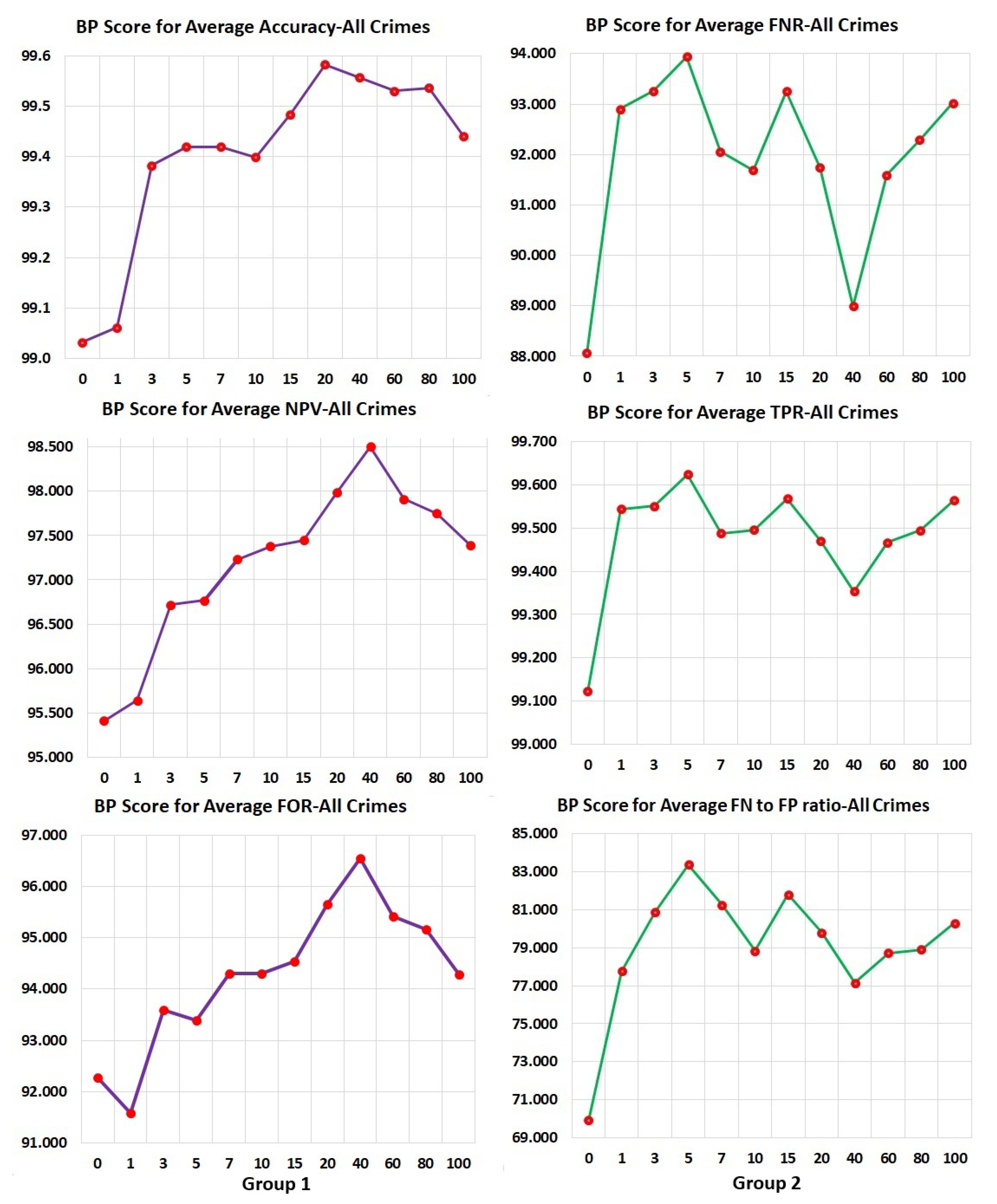
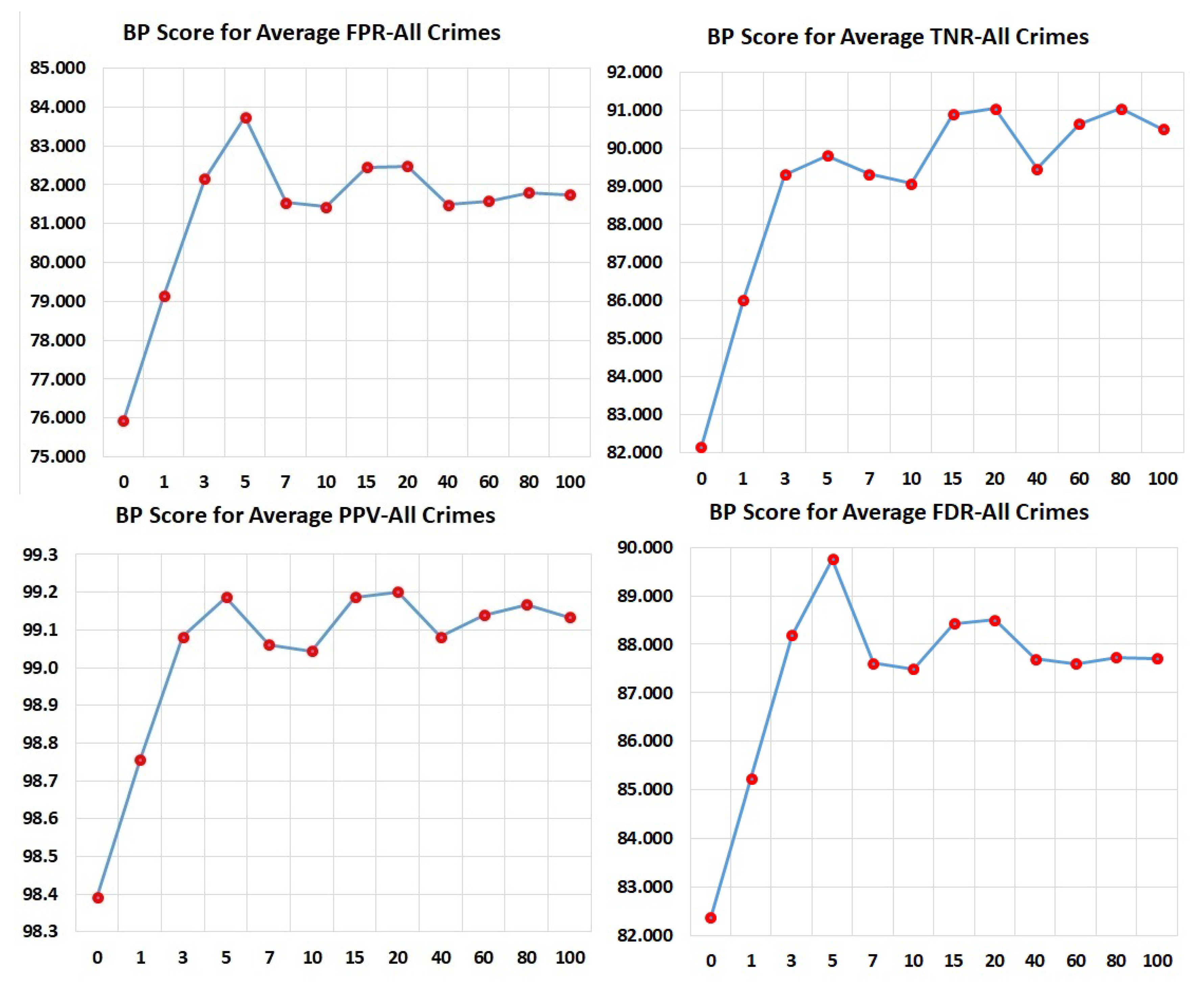
To further study the effect of the number of arrest cycles on the BP scores for the different statistical measures, Figure 1 and Figure 2 show the BP scores plotted against the number of arrest cycles used. These graphs show two important observations, namely (i) that for all measures the inclusion of past arrest records in the data significantly improved the fairness (i.e., the BP score), and (ii) that for different measures the detailed relation of arrest cycles to BP score behaved differently. In particular, behavior seemed to fall into one of three groups, indicated with different colored graphs in the figures. In the first of these groups (comprising ACC, NPV, and FOR), fairness increased until around 40 arrest cycles and then dropped. In the second group (comprising FNR, TPR, and FN to FP ratio), fairness (BP score) peaked at five arrest cycles and then dropped slightly, while in the third group (comprising FPR, TNR, PPV, and FDR), fairness reached close to highest performance again at five cycles and then stayed relatively constant. These results suggest that we can use the desired balance of measures to pick the least biased model for later use, In this case, since we will compare against systems that largely evaluated their models in terms of FPR, FNR, TPR, and TNR, we selected our model with five prior arrest cycles for the comparison shown in Table 7. More detailed discussion of the results and observations are provided in Section 6 and Section 7.
6. Performance Evaluation
To evaluate the overall performance of our model, we compare the performance of our lowest bias model with the results of two previous papers that used the same dataset.
The work by Ozkan [34] utilized six classifiers, namely, Logistic Regression, Random Forests, XG-Boost, Support Vector Machines, Neural Networks, and Search algorithms on the same dataset as used in this work. Just like Zeng et al. [32], they used only the 1994 records for training and test purposes while we used all arrests cycles for training and testing purposes. Zeng et al. [32] used rearrests as representative of recidivism while [34] the current work uses reconvictions as indicators of recidivism. Though the previous two works used some history, we use a more detailed history that takes the rolling sum of 26 different types of crimes, substance abuse and courses taken into consideration for each cycle.
The work by Ozkan [34] achieved the best results for Accuracy using XGBoost at 0.778, for FPR and TNR using Logistic Regression at 0.406 and 0.594, respectively, and for FNR and TPR using SVM at 0.054 and 0.946, respectively. For our comparison, we will use these best scores even though they are not achieved by one consistent model and can thus not be achieved simultaneously by their system.
In contrast to the comparison data from Oskan, we used a single model for all of the performance results for our model by picking the model with the lowest average bias in all the comparison categories which turned out to be the one considering five past arrest cycles. The classifier trained here is a single neural network as described in Section 5 and thus achieves all comparison results simultaneously. This model achieved an accuracy of 0.892, FPR of 0.378, FNR of 0.056, TPR of 0.944, and TNR of 0.622. Comparing this with Ozkan’s results shows that our model achieves significantly higher accuracy while obtaining better FPR and TNR, with approximately equivalent FNR and TPR compared to their best values in each of the categories.
Zeng et al. [32], who were pursuing transparency rather than accuracy or reduction of bias, achieved a mean five-fold cross-validation TPR and FPR of 78.3% and 46.5%, respectively, while we achieved 94.4% and 37.8% for these metrics using a 10-fold Monte Carlo cross-validation, thus significantly improving in both measures.
Neither of the comparisons directly evaluated a single fairness score and their results are thus optimized irrespective of fairness across groups. To test that our model can not only achieve better performance but also fairer predictions, we evaluated the BP scores. The achieved BP scores of 99.4 for Accuracy, 83.7 for FPR, 93.9 for FNR, 99.6 for TPR, and 89.8 for TNR show that our system succeeded at obtaining high levels of parity in all of the metrics. See Table 7 for the complete comparison.
7. Results and Discussion
We used a three-layer deep learning neural network on a recidivism dataset. The dataset had more Caucasian records than African American records. However, the African American offenders had more rearrests than Caucasians. As a result, when we split the original offender 1994 release records that included up to 99 prior and/or subsequent arrest records to create multiple records, each with a single arrest and subsequent release information, there were more African American records than Caucasian records. When we used neural networks to predict recidivism without each prior arrest’s history being included in the records, the results had significant bias embedded in them. The inclusion of information from past arrests increased accuracy and reduced bias. We conducted experiments by including history information from 0, 1, 3, 5, 7, 10, 15, 20, 40, 60, 80, and 100 past arrest cycle records. This increased the accuracy and decreased the bias using the various given metrics. We used BP Score for each metric for each of the given sets of experiments and found that for most metrics, the model generated with the data using the past five arrest cycles’ information had the least bias. See Table 1, Table 2, Table 3, Table 4, Table 5 and Table 6 for the detailed results of the different models. If it was not the least bias, it was close to the least bias amongst the given BP scores.
The results from processing the raw data without a prior history, even in the absence of race, designates more recidivism labels to non-recidivating African Americans (higher FPR) than to non-recidivating Caucasians (lower FPR). Furthermore, it assigns fewer non-recidivating labels to recidivating African Americans (lower FNR) and more non-recidivating labels to recidivating Caucasians (higher FNR). This trend was reduced as we included a rolling sum of 26 types of individual crimes, substance abuse, and courses and treatments taken during incarceration for 0, 1, 3, 5, 7, 15, 20, 40, 60, 80, and 100 past arrest records. We can determine if a classifier is fair by using the BP Score that compares metric values for the different subpopulations. Only a practitioner can decide whether having a given BP Score, for example 90, for all or a subset of the fairness metrics can be considered fair or the model needs to be improved further. As the quality of data improves and the ethical standards of our society are raised, we assume that society will continue to demand an ever-increasing value of the BP score, until it is close to a near-perfect 100. The BP score can allow a practitioner to identify bias in a model using different statistical measures, where 100 and 0 are the best and the worst values, respectively. In recidivism, high FPR means more non-recidivists will have to languish in jail while a high FNR means that society is at risk, because recidivists are being let out of jail. A parole officer may decide to use BPS for both Accuracy and FPR above 90 and for FNR above 80. On the other hand, a loan officer may use a minimum BPS for false-negative error rate balance (Equal Opportunity) [14,15] for a model to determine the loan worthiness of a client. Any new fairness measures that may evolve after this paper can also use BP Scores to determine the bias embedded in models and choose the one with the highest BPS or the least bias amongst the given models.
We plotted BP Scores for different metrics based on models created using different numbers of past arrest cycle details (0, 1, 3, 5, 7, 10, 15, 20, 40, 60, 80, 100 prior arrests). We saw our BP Scores fall into three groups as shown in Figure 1 and Figure 2: Group 1 is comprised of BPS-Average Accuracy, BPS-Average Negative Predicted Value, and BPS-Average False Omission Rate. This group experiences a steady increase in BPS until around 40 past arrest cycles of information. This means that considering long histories improve these metric values until only very few individuals are in the long history category, upon which fairness suffers (BPS goes down). Group 2 consists of BPS-Average False-Negative rate, BPS-Average True-Positive Rate, and BPS-Average FN-to-FP-ratio (Treatment Equality). For these metrics, short histories are beneficial but then have significant dips in BP scores with additional history. This means that long histories can produce significant bias issues in Average False-Negative Rates, Average True-Positive Rates, and Average False-Negative to False-Positive Rates (Treatment Equality). Group 3 is comprised of BPS-Average False-Positive Rate, BPS-Average True -Negative Rate, BPS-Average Positive Predictive Value, and Average False Discovery Rate. These show similar effects as Group 2 early on. This group shows a rapid increase in BP score by adding a little bit of history but is then largely unaffected when increasing the history further. As a result of looking at the BP scores, especially for Group 2, we chose the model created with information from five past arrest cycles. This model minimizes bias reflected in most metrics used in this work. A decision maker can use BPS similarly. Averages have been calculated using 10 fold Monte Carlo cross-validation.
8. Limitations
We have used the “Recidivism of Prisoners Released in 1994” [19] dataset and our work is limited by the data provided in it, which in turn is limited by the time frame for which data is captured. Prisoner records for up to 1997 (and in some cases beyond 1997) have been included in the dataset. We have utilized all of these in our experiments. It is possible that a number of individuals committed crimes after 1997 but their criminal activities were not included in the dataset. Additionally, race is stored in our dataset as a discrete value. We have accordingly assumed racial disjointness of the offenders, as done in substantial amounts of the related literature, including [11,24,32,34] and many more. However, demographic groups intersect and it is likely that mixed-race offenders are recorded as only one of the races. Furthermore, we use re-conviction as an indicator of recidivism, as opposed to using re-arrest, as frequent re-arrest could be indicative of human bias. However, if there was human bias in the reconviction decisions, algorithmic decisions will embody them, too.
9. Conclusions
In this paper, we used a three-layered neural network classifier to train a recidivism predictor and computed several statistical measures (defined in Section 4 and in the Appendix A) for a recidivism dataset and demonstrated how these can be used to compute the fairness of a prediction model. We introduced a new metric called BP score, which quantifies the bias in models and allows easy comparison of model results to identify the one with the least bias. The original recidivism dataset was comprised of one record per offender, where each record was a 1994 release record and included up to 99 prior and/or subsequent arrest-release records in each record. We used each record to mint multiple records, each comprised of a single arrest and subsequent release event. We then made multiple models, enriched with features containing different numbers of past arrest cycles and related offenders’ criminal history, substance abuse history and any courses or treatments taken during incarceration. We demonstrate that by adding personal history we could increase prediction accuracy and measurably decrease bias. We demonstrate how to use BP score to measure reduction in bias using any of the statistical measures described in the paper. Using the metric BP score for the demonstration of the quantitative measure of the reduction of bias using one number is an important contribution of this paper because BP score can be used to compare bias embedded in multiple models and can be used with any underlying statistical measure. Using past history to increase prediction accuracy and decrease bias is important because similar techniques can be applied to applications in many domains like dating, loan application acceptance, hiring, granting parole, insurance coverage, and medical diagnosis as each of these have related history.
10. Future Work
As machine learning-based decision support systems continue to be deployed in many domains, the bias and fairness of their results have become significantly pertinent for our world. As a result, the need to alleviate bias in the resulting predictive models has become increasingly important to keep our world fair. The impact of our work is very broad and can be applied in multiple areas such as medical diagnosis, loan application acceptance, dating, hiring, etc. Furthermore, many sensitive attributes such as gender, race, age, income, weight, zip code, mental health status, etc. [10,11] can influence the unfairness in prediction results. Their effects in different domains can be studied and mitigated with the methodology used in this work. In the current work, we developed an approach to adding history to the input vector that increased accuracy of prediction models. Yet another contribution of the current work is the fairness measure BP score that can be used to quantify bias in the prediction models for different statistical measures. Both of these lead us to multiple directions of future work.
So far we have applied the approach to predict total crimes. Using the enriched recidivism dataset we could predict the three most serious crimes committed after release on parole as the current dataset stores three most serious crimes committed in each arrest-release cycle. This would allow more detailed predictions and should be followed up by measuring bias in these enhanced prediction models.
When making more complex predictions for different crime categories, it might become important to develop new measures to measure the accuracy of multiple types of concurrent crimes (outcomes) in the prediction model that could also consider the severity of the individual crimes. This should be followed up by creating corresponding models, verifying their accuracy and efficacy, and evaluating the presence of bias in them.
While the current work only uses the BP scores to select a model, it does not use them to modify the training of the model. To address this we are planning to develop different BP Score-based loss functions, namely FPR-BPS, FNR-BPS, TPR-BPS, TNR-BPS, FPR-FNR-BPS, and TPR-TNS-BPS, to train models with multiple recidivism-based datasets. The bias in the resulting models could be measured using BP Scores for the pertinent statistical measures to see if even better models can be achieved when explicitly pursuing fairness during training.
We could apply similar techniques to first enrich datasets from dating, hiring, medical diagnosis, and other domains, followed by measuring bias in these models with BP score. Similarly, we could consider applying these techniques in the context of a broader range of potential factors for bias, using them to reduce age, income, weight, zip code, or mental health status-based bias in other domains.
Author Contributions
The individual contributions were as follows: conceptualization/original draft preparation/writing/visualization, B.J., methodology/formal analysis/review/resources, B.J. and M.H.; co-supervision, R.E., and L.F. All authors have read and agreed to the published version of the manuscript.
Funding
This research received no external funding.
Conflicts of Interest
The authors declare no conflict of interest.
Abbreviations
The following abbreviations are used throughout this paper:
| ACC | Accuracy |
| BPS | Bias Parity Score |
| FN | False-Negative |
| FDR | False Discovery Rate |
| FNR | False-Negative Rate |
| FOR | False Omission Rate |
| FP | False-Positive |
| FPR | False-Positive Rate |
| NPV | Negative Predictive Value |
| S.P. | Statistical Parity |
| T.E. | Treatment Equality |
| TN | True-Negative |
| TNR | True-Negative Rate |
| TP | True-Positive |
| TPR | True-Positive Rate |
Appendix A
This appendix provides an explanation of the notation along with the list of definitions and related formulas of several statistical measures used throughout the paper.
Notation: We use the notation included in this section to formulate the problem of predicting recidivism with a single sensitive attribute of race. We need to find the model that helps predict with high accuracy and lowest bias possible amongst the given models, each one of which is developed with the rolling sum of prior individual crimes from N prior arrest records.
- : quantified features of each elemnt in the dataset.
- : Race-based binary sensitive attribute (African American, Caucasian)
- : predicted variable (not reconvicted/reconvicted)
- : target variable (will not reoffend/will reoffend).
- Assumption: (X, A, Y) are generated from a distribution d denoted as
- measure(A′): value of a metric for subpopulation with A = 0.
- measure(A) : value of a metric for subpopulation with A = 1.
TP: True-Positive (TP) is a correct positive prediction. In our paper it means that a future recidivist was correctly forecasted to recidivate.
TN: True-Negative (TN) is a correct negative prediction. In our paper it means that a future non-recidivist was correctly forecasted to not recidivate.
FP: False-Positive (FP) is an incorrect positive prediction, when a future nonrecidivist was falsely forecasted to recidivate.
FN: False-Negatives (FN) is an incorrect negative prediction. In our paper it means that a future recidivist was erroneously labeled as nonrecidivist.
Positive Predictive Value: PPV, also referred to as Precision, is the total number of true-positive cases divided by a total of all predicted positive cases. The best possible value of PPV is 1 and is achieved when FP becomes zero, i.e., when none of the future non-recidivists are wrongly accused of being a recidivist. The worst value of PPV is 0 and happens when none of the individuals predicted to recidivate are actually recidivists, i.e., when TP is zero. Therefore, it is desirable to have PPV as close to 1 as possible. PPV also refers to the probability of an offender to truly belong to the positive class, and . PPV parity [14] is achieved when . Average PPV and BPS for the model with 5 past arrest cycles and all race data were 0.853 and 97.9, respectively.
False-Positive Rate: FPR is the total number of incorrect positive predictions divided by a total of all the non-recidivists (FP + TN) in the dataset. The best possible value of FPR is 0 and is achieved when FP becomes zero, i.e., none of the future non-recidivists are wrongly accused of being a recidivist. The worst value of FPR is 1 and happens when all future non-recidivists are falsely labeled as recidivists such that TN becomes 0. Therefore, it is desirable to have FPR as close to 0 as possible. FPR is represented as and .
FPR parity or false-positive error rate balance [14] or predictive equality [40] is achieved when . Average FPR and BPS for the model with 5 past arrest cycles and all race data were 0.378 and 83.7, respectively.
False-Negative Rate: FNR is the total number of incorrect negative predictions divided by a total of all the recidivists (FN + TP) in the dataset. The best possible value of FNR is 0 and is achieved when FN becomes zero, i.e., none of the future recidivists are erroneously labeled as a non-recidivist. The worst value of FNR is 1 and happens when all future recidivists are falsely labeled as non-recidivists such that TP becomes 0. FNR is represented as and FNR parity is achieved when . Average FNR and BPS for the model with 5 past arrest cycles and all race data were 0.056 and 93.9, respectively.
It is desirable to have both FPR and FNR as close to 0 as possible. A high FPR represents many future non-recidivists wasting behind bars while a high FNR means many future recidivists let lose to commit many needless crimes in the world. Both FPR and FNR mean different types of error and associated cost to society. Both higher FPR and higher FNR cause a decrease in the predictive accuracy.
False Discovery Rate: FDR is the total number of incorrect positive predictions (FP) divided by a total of all positive predictions (TP + FP). The best possible value of FDR is 0 and is achieved when FP becomes zero, i.e., none of the future non-recidivists are mislabeled as recidivist. The worst value of FOR is 1 and happens when all future recidivists are falsely labeled as non-recidivists such that TP becomes 0. Therefore, it is desirable to have FDR as close to 0 as possible. FDR refers to the probability of a positively labeled individual to actually belong to the negative class, , or the probability of a person kept incarcerated to be a non-recidivist. and . FDR parity is achieved when Average FDR and BPS for the model with 5 past arrest cycles and all race data were 0.071 and 89.8, respectively.
False Omission Rate: FOR is the total number of incorrect negative predictions (FN) divided by a total of all predicted non-recidivists (TN + FN). The best possible value of FOR is 0 and is achieved when FN becomes zero, i.e., none of the future recidivists are mislabeled as non-recidivist and let go. The worst value of FOR is 1 and happens when all future non-recidivists are falsely labeled as recidivists such that TN becomes 0. Therefore, it is desirable to have FOR as close to 0 as possible. FOR refers to the probability of a positive class to be labeled negatively, (P(Y = 1 |C = 0), or the probability of a someone who is let go to be a recidivist. . FOR parity is achieved when Average FOR and BPS for the model with 5 past arrest cycles and all race data were 0.323 and 93.4, respectively.
Negative Predictive Value: NPV is the total number of true-negatives divided by the total number of negative predictions. The best possible value of NPV is 1. The worst value of NPV is 0 when all negative class are predicted to be positive class such that FN =0. NPV refers to the probability of a negative prediction to truly belong to the negative class, , or the probability of someone predicted to be a non-recidivist to actually be a non-recidivist. and . NPV parity is achieved when . Average NPV and BPS for the model with 5 past arrest cycles and all race data were 0.677 and 96.8, respectively.
True-Positive Rate: TPR is the total number of true-positive cases identified divided by the total number of positive cases. The best possible value of TPR is 1 and is achieved when FN is equal to 0. TPR, also known as sensitivity or recall, is the probability of the positive class to be labeled as positive, or the probability of a recidivist to be labeled as one. and . TPR parity is achieved when . Average TPR and BPS for the model with 5 past arrest cycles and all race data were 0.944 and 99.6, respectively.
True-Negative Rate: TNR is the total number of correctly labeled negative predictions divided by all the negative cases. The best possible value of TNR is 1 and is achieved when FP is 0. TNR refers to the probability of a negative class being labeled negative, This in our predictions is the probability of non-recidivists being labeled a non-recidivist. and . TNR parity is achieved when . Average TNR and BPS for the model with 5 past arrest cycles and all race data were 0.622 and 89.8, respectively.
Accuracy: Accuracy is the total number of appropriately labeled predictions divided by the number of all the cases. The best possible value of Accuracy is 1 and is achieved when both FP and FN are 0. Accuracy refers to the probability of accurate labeling for both positive and negative classes, P(C = Y). This in our predictions is the probability of being correctly labeled as a recidivist or non-recidivist as the case is. and . Accuracy parity is achieved when . Average Accuracy and BPS for the model with 5 past arrest cycles and all race data were 0.892 and 99.4 respectively.
Statistical Parity or Group Fairness or Demographical Parity [15] or Equal Acceptance Rate [41] is the property that the demographics of those labeled with a positive (or negative) classifications is the same as the demographics of the population as a whole [15]. In other words, this is true if all subgroups have equal probability to be labeled as the positive class [12]. and and and the condition is satisfied. The fraction of all positive predicted cases from all cases and BPS (statistical parity) for the model with 5 past arrest cycles and all race data were 0.854 and 97.9, respectively.
The situation may be unfair for an individual even as statistical parity is accomplished. As per Dwork et al. [15], this can provide fair affirmative action but may be insufficient in other situations, e.g., if one subgroup has in fact more members with positive class than the other group or when more unqualified members are chosen to fulfill the condition [15]. In our dataset, it is used to give members of different races a possibility of parole but this may not be fair if one group reoffends more.
Treatment Equality [13] or false-negative-to-false-positive ratio is achieved when the ratio of errors, i.e., false-negatives and false-positives for the subpopulations are equal, such that and and the condition is satisfied. In our dataset this means that for both African-Americans and Caucasians, the ratio of recidivists labeled as non-recidivists (FN) to non-recidivists labeled as recidivists should be the same. The average fraction of all false-negative cases to false-positive cases from all cases and BPS (Treatment Equality) for the model with five past arrest cycles and all race data were 0.798 and 83.8, respectively.
References
- Nelson, G.S. Bias in artificial intelligence. N. Carol. Med. J. 2019, 80, 220–222. [Google Scholar] [CrossRef] [PubMed]
- Ahsen, M.E.; Ayvaci, M.U.S.; Raghunathan, S. When algorithmic predictions use human-generated data: A bias-aware classification algorithm for breast cancer diagnosis. Inf. Syst. Res. 2019, 30, 97–116. [Google Scholar] [CrossRef]
- He, H.; Nawata, K. The Application of Machine Learning Algorithms in Predicting the Borrower’s Default Risk in Online Peer-to-Peer Lending. 2019. Available online: https://webofproceedings.org/proceedings_series/ESSP/ICEMIT%202019/ICEMIT19016.pdf (accessed on 8 November 2020).
- Suarez-Tangil, G.; Edwards, M.; Peersman, C.; Stringhini, G.; Rashid, A.; Whitty, M. Automatically dismantling online dating fraud. IEEE Trans. Inf. Forensics Secur. 2019, 15, 1128–1137. [Google Scholar] [CrossRef] [Green Version]
- Mahmoud, A.A.; Shawabkeh, T.A.; Salameh, W.A.; Al Amro, I. Performance Predicting in Hiring Process and Performance Appraisals Using Machine Learning. In Proceedings of the 2019 10th International Conference on Information and Communication Systems (ICICS), Oxford, UK, 11–13 June 2019; pp. 110–115. [Google Scholar]
- Johndrow, J.E.; Lum, K. An algorithm for removing sensitive information: Application to race-independent recidivism prediction. Ann. Appl. Stat. 2019, 13, 189–220. [Google Scholar] [CrossRef] [Green Version]
- Baudry, M.; Robert, C.Y. A machine learning approach for individual claims reserving in insurance. Appl. Stoch. Model. Bus. Ind. 2019, 35, 1127–1155. [Google Scholar] [CrossRef]
- Akbani, R.; Kwek, S.; Japkowicz, N. Applying support vector machines to imbalanced datasets. In Proceedings of the European Conference on Machine Learning, Pisa, Italy, 20–24 September 2004; pp. 39–50. [Google Scholar]
- Hajian, S.; Bonchi, F.; Castillo, C. Algorithmic bias: From discrimination discovery to fairness-aware data mining. In Proceedings of the 22nd ACM SIGKDD International Conference on Knowledge Discovery and Data Mining, San Francisco, CA, USA, 13–17 August 2016; pp. 2125–2126. [Google Scholar]
- FitzGerald, C.; Hurst, S. Implicit bias in healthcare professionals: A systematic review. BMC Med. Ethics 2017, 18, 19. [Google Scholar] [CrossRef] [PubMed] [Green Version]
- Dressel, J.; Farid, H. The accuracy, fairness, and limits of predicting recidivism. Sci. Adv. 2018, 4, eaao5580. [Google Scholar] [CrossRef] [PubMed] [Green Version]
- Verma, S.; Rubin, J. Fairness definitions explained. In Proceedings of the 2018 IEEE/ACM International Workshop on Software Fairness (FairWare), Gothenburg, Sweden, 29 May 2018; pp. 1–7. [Google Scholar]
- Berk, R.; Heidari, H.; Jabbari, S.; Kearns, M.; Roth, A. Fairness in criminal justice risk assessments: The state of the art. Sociol. Methods Res. 2018, 2018, 0049124118782533. [Google Scholar] [CrossRef]
- Chouldechova, A. Fair prediction with disparate impact: A study of bias in recidivism prediction instruments. Big Data 2017, 5, 153–163. [Google Scholar] [CrossRef] [PubMed]
- Dwork, C.; Hardt, M.; Pitassi, T.; Reingold, O.; Zemel, R. Fairness through awareness. In Proceedings of the 3rd Innovations in Theoretical Computer Science Conference, Cambridge, MA, USA, 8–10 January 2012; pp. 214–226. [Google Scholar]
- Hardt, M.; Price, E.; Srebro, N. Equality of opportunity in supervised learning. In Proceedings of the Advances in Neural Information Processing Systems, Barcelona, Spain, 5–10 December 2016; pp. 3315–3323. [Google Scholar]
- Kusner, M.J.; Loftus, J.; Russell, C.; Silva, R. Counterfactual fairness. In Proceedings of the Advances in Neural Information Processing Systems, Long Beach, CA, USA, 4–9 December 2017; pp. 4066–4076. [Google Scholar]
- Mehrabi, N.; Morstatter, F.; Saxena, N.; Lerman, K.; Galstyan, A. A survey on bias and fairness in machine learning. arXiv 2019, arXiv:1908.09635. [Google Scholar]
- United States Department of Justice, Office of Justice Programs, Bureau of Justice Statistics. Recidivism of Prisoners Released in 1994. Available online: https://www.icpsr.umich.edu/icpsrweb/NACJD/studies/3355/variables (accessed on 5 December 2014).
- Barocas, S.; Selbst, A.D. Big data’s disparate impact. Calif. Law Rev. 2016, 104, 671. [Google Scholar] [CrossRef]
- Miron, M.; Tolan, S.; Gómez, E.; Castillo, C. Evaluating causes of algorithmic bias in juvenile criminal recidivism. Artif. Intell. Law 2020, 2020, 1–37. [Google Scholar] [CrossRef]
- Jung, J.; Goel, S.; Skeem, J. The limits of human predictions of recidivism. Sci. Adv. 2020, 6, eaaz0652. [Google Scholar]
- Zafar, M.B.; Valera, I.; Gomez Rodriguez, M.; Gummadi, K.P. Fairness beyond disparate treatment & disparate impact: Learning classification without disparate mistreatment. In Proceedings of the 26th International Conference onWorldWide Web, Perth, Australia, 3–7 May 2017; pp. 1171–1180. [Google Scholar]
- Angwin, J.; Larson, J.; Mattu, S.; Kirchner, L. Machine bias: There’s software used across the country to predict future criminals. And it’s biased against blacks. ProPublica 2016, 2016, 23. [Google Scholar]
- Jain, B.; Huber, M.; Fegaras, L.; Elmasri, R.A. Singular race models: Addressing bias and accuracy in predicting prisoner recidivism. In Proceedings of the 12th ACM International Conference on PErvasive Technologies Related to Assistive Environments, Rhodes, Greece, 5–7 June 2019; pp. 599–607. [Google Scholar]
- Jain, B.; Huber, M.; Elmasri, R.A.; Fegaras, L. Reducing race-based bias and increasing recidivism prediction accuracy by using past criminal history details. In Proceedings of the 13th ACM International Conference on PErvasive Technologies Related to Assistive Environments, New York, NY, USA, 13–15 June 2020; pp. 1–8. [Google Scholar]
- Feldman, M.; Friedler, S.A.; Moeller, J.; Scheidegger, C.; Venkatasubramanian, S. Certifying and removing disparate impact. In Proceedings of the 21th ACM SIGKDD International Conference on Knowledge Discovery and Data Mining, Sydney, Australia, 10–13 August 2015; pp. 259–268. [Google Scholar]
- Luong, B.T.; Ruggieri, S.; Turini, F. k-NN as an implementation of situation testing for discrimination discovery and prevention. In Proceedings of the 17th ACM SIGKDD International Conference on Knowledge Discovery and Data Mining, San Diego, CA, USA, 21–24 August 2011; pp. 502–510. [Google Scholar]
- Zemel, R.; Wu, Y.; Swersky, K.; Pitassi, T.; Dwork, C. Learning fair representations. In Proceedings of the International Conference on Machine Learning, Atlanta, GA, USA, 16–21 June 2013; pp. 325–333. [Google Scholar]
- Biswas, A.; Kolczynska, M.; Rantanen, S.; Rozenshtein, P. The Role of In-Group Bias and Balanced Data: A Comparison of Human and Machine Recidivism Risk Predictions. In Proceedings of the 3rd ACM SIGCAS Conference on Computing and Sustainable Societies, Guayaquil, Ecuador, 15–17 June 2020; pp. 97–104. [Google Scholar]
- Chouldechova, A.; Roth, A. The frontiers of fairness in machine learning. arXiv 2018, arXiv:1810.08810. [Google Scholar]
- Zeng, J.; Ustun, B.; Rudin, C. Interpretable classification models for recidivism prediction. J. R. Stat. Soc. Ser. A 2017, 180, 689–722. [Google Scholar] [CrossRef]
- Chen, I.; Johansson, F.D.; Sontag, D. Why is my classifier discriminatory? In Proceedings of the Advances in Neural Information Processing Systems, Montreal, QC, Canada, 3–8 December 2018; pp. 3539–3550. [Google Scholar]
- Ozkan, T. Predicting Recidivism Through Machine Learning. Ph.D. Thesis, Stanford University, Stanford, CA, USA, 2017. [Google Scholar]
- Calders, T.; Verwer, S. Three naive Bayes approaches for discrimination-free classification. Data Min. Knowl. Discov. 2010, 21, 277–292. [Google Scholar] [CrossRef] [Green Version]
- Krasanakis, E.; Spyromitros-Xioufis, E.; Papadopoulos, S.; Kompatsiaris, Y. Adaptive sensitive reweighting to mitigate bias in fairness-aware classification. In Proceedings of the 2018 World Wide Web Conference, Lyon, France, 23–27 April 2018; pp. 853–862. [Google Scholar]
- Biddle, D. Adverse Impact and Test Validation: A Practitioner’s Guide to Valid and Defensible Employment Testing; Gower Publishing, Ltd.: Aldershot, UK, 2006. [Google Scholar]
- US Equal Employment Opportunity Commission. Questions and Answers to Clarify and Provide a Common Interpretation of the Uniform Guidelines on Employee Selection Procedures; US Equal Employment Opportunity Commission: Washington, DC, USA, 1979.
- Won, H.R.; Shim, J.S.; Ahn, H. A Recidivism Prediction Model Based on XGBoost Considering Asymmetric Error Costs. J. Intell. Inf. Syst. 2019, 25, 127–137. [Google Scholar]
- Corbett-Davies, S.; Pierson, E.; Feller, A.; Goel, S.; Huq, A. Algorithmic decision making and the cost of fairness. In Proceedings of the 23rd ACM Sigkdd International Conference on Knowledge Discovery and Data Mining, Halifax, NS, Canada, 13–17 August 2017; pp. 797–806. [Google Scholar]
- Zliobaite, I. On the relation between accuracy and fairness in binary classification. arXiv 2015, arXiv:1505.05723. [Google Scholar]
Figure 1.
Bias Parity Score (BPS) by number of past arrest-release cycles (0, 1, 3, 5, 7, 10, 15, 20, 40, 60, 80, 100). Group 1: BPS-Avg. Accuracy, BPS-Avg. Negative Predicted Value, BPS-Avg. False Omission Rate. Group 2: BPS-Avg. False-Negative rate, BPS-Avg. True-Positive Rate, BPS-Avg. FN-to-FP-ratio. Averages: Computed using 10 iterations of Monte Carlo cross-validation.

Figure 2.
BP Scores by number of past arrest-release cycles (0, 1, 3, 5, 7, 10, 15, 20, 40, 60, 80, 100). Group 3: BPS-Avg.False-Positive Rate, BPS-Avg. True-Negative Rate, BPS-Avg. Positive Predictive Value, Avg.False Discovery Rate. Averages: Computed using 10 iterations of Monte Carlo cross-validation.


Table 1.
Average accuracy.
| Arrest Cycles | All Races Train/Test | All Races Train, Test Caucasian | All Races Train, Test Afr. Amer. | BPS |
|---|---|---|---|---|
| 0 | 0.879 | 0.883 | 0.875 | 99.032 |
| 1 | 0.888 | 0.893 | 0.884 | 99.062 |
| 3 | 0.891 | 0.894 | 0.888 | 99.383 |
| 5 | 0.892 | 0.895 | 0.890 | 99.419 |
| 7 | 0.894 | 0.897 | 0.892 | 99.420 |
| 10 | 0.896 | 0.899 | 0.894 | 99.399 |
| 15 | 0.898 | 0.900 | 0.896 | 99.484 |
| 20 | 0.899 | 0.901 | 0.897 | 99.583 |
| 40 | 0.899 | 0.902 | 0.898 | 99.557 |
| 60 | 0.900 | 0.902 | 0.898 | 99.530 |
| 80 | 0.899 | 0.902 | 0.897 | 99.536 |
| 100 | 0.899 | 0.902 | 0.897 | 99.440 |
Table 2.
Average positive predictive rate.
| Arrest Cycles | All Races Train/Test | All Races Train, Test Caucasian | All Races Train, Test Afr. Amer. | BPS |
|---|---|---|---|---|
| 0 | 0.853 | 0.838 | 0.867 | 96.645 |
| 1 | 0.857 | 0.843 | 0.865 | 97.412 |
| 3 | 0.848 | 0.838 | 0.858 | 97.740 |
| 5 | 0.853 | 0.844 | 0.862 | 97.915 |
| 7 | 0.849 | 0.838 | 0.858 | 97.657 |
| 10 | 0.852 | 0.842 | 0.862 | 97.648 |
| 15 | 0.847 | 0.835 | 0.855 | 97.717 |
| 20 | 0.844 | 0.835 | 0.854 | 97.779 |
| 40 | 0.853 | 0.842 | 0.863 | 97.544 |
| 60 | 0.845 | 0.835 | 0.854 | 97.716 |
| 80 | 0.842 | 0.832 | 0.851 | 97.773 |
| 100 | 0.846 | 0.836 | 0.855 | 97.804 |
Table 3.
Average false-positive rate.
| Arrest Cycles | All Races Train/Test | All Races Train, Test Caucasian | All Races Train, Test Afr. Amer. | BPS |
|---|---|---|---|---|
| 0 | 0.417 | 0.360 | 0.474 | 75.938 |
| 1 | 0.393 | 0.347 | 0.438 | 79.134 |
| 3 | 0.366 | 0.330 | 0.401 | 82.150 |
| 5 | 0.378 | 0.344 | 0.411 | 83.742 |
| 7 | 0.357 | 0.321 | 0.393 | 81.542 |
| 10 | 0.362 | 0.324 | 0.398 | 81.433 |
| 15 | 0.333 | 0.300 | 0.364 | 82.448 |
| 20 | 0.329 | 0.297 | 0.360 | 82.481 |
| 40 | 0.354 | 0.317 | 0.389 | 81.496 |
| 60 | 0.327 | 0.293 | 0.359 | 81.591 |
| 80 | 0.320 | 0.287 | 0.351 | 81.798 |
| 100 | 0.333 | 0.299 | 0.365 | 81.751 |
Table 4.
Average true-negative rate.
| Arrest Cycles | All Races Train/Test | All Races Train, Test Caucasian | All Races Train, Test Afr. Amer. | BPS |
|---|---|---|---|---|
| 0 | 0..583 | 0.640 | 0.526 | 82.156 |
| 1 | 0.607 | 0.653 | 0.562 | 86.016 |
| 3 | 0.634 | 0.670 | 0.599 | 89.308 |
| 5 | 0.622 | 0.656 | 0.589 | 89.810 |
| 7 | 0.643 | 0.679 | 0.607 | 89.320 |
| 10 | 0.638 | 0.676 | 0.602 | 89.072 |
| 15 | 0.664 | 0.700 | 0.636 | 90.881 |
| 20 | 0.671 | 0.703 | 0.640 | 91.041 |
| 40 | 0.646 | 0.683 | 0.611 | 89.456 |
| 60 | 0.673 | 0.707 | 0.641 | 90.637 |
| 80 | 0.680 | 0.713 | 0.649 | 91.041 |
| 100 | 0.667 | 0.701 | 0.635 | 90.492 |
Table 5.
Average false-negative rate.
| Arrest Cycles | All Races Train/Test | All Races Train, Test Caucasian | All Races Train, Test Afr. Amer. | BPS |
|---|---|---|---|---|
| 0 | 0.059 | 0.069 | 0.061 | 88.059 |
| 1 | 0.058 | 0.061 | 0.056 | 92.904 |
| 3 | 0.060 | 0.063 | 0.059 | 93.262 |
| 5 | 0.56 | 0.059 | 0.055 | 93.938 |
| 7 | 0.058 | 0.061 | 0.056 | 92.058 |
| 10 | 0.055 | 0.057 | 0.053 | 91.688 |
| 15 | 0.058 | 0.060 | 0.056 | 93.258 |
| 20 | 0.058 | 0.061 | 0.056 | 91.740 |
| 40 | 0.053 | 0.056 | 0.050 | 88.990 |
| 60 | 0.057 | 0.060 | 0.055 | 91.598 |
| 80 | 0.059 | 0.062 | 0.057 | 92.288 |
| 100 | 0.057 | 0.059 | 0.055 | 93.019 |
Table 6.
Average true-positive rate.
| Arrest Cycles | All Races Train/Test | All Races Train, Test Caucasian | All Races Train, Test Afr. Amer. | BPS |
|---|---|---|---|---|
| 0 | 0.935 | 0.931 | 0.939 | 99.123 |
| 1 | 0.942 | 0.939 | 0.944 | 99.544 |
| 3 | 0.940 | 0.937 | 0.941 | 99.551 |
| 5 | 0.944 | 0.941 | 0.945 | 99.624 |
| 7 | 0.942 | 0.939 | 0.944 | 99.488 |
| 10 | 0.945 | 0.943 | 0.947 | 99.496 |
| 15 | 0.942 | 0.940 | 0.944 | 99.568 |
| 20 | 0.942 | 0.939 | 0.944 | 99.470 |
| 40 | 0.947 | 0.944 | 0.950 | 99.353 |
| 60 | 0.943 | 0.940 | 0.945 | 99.467 |
| 80 | 0.941 | 0.938 | 0.943 | 99.495 |
| 100 | 0.943 | 0.941 | 0.945 | 99.565 |
Publisher’s Note: MDPI stays neutral with regard to jurisdictional claims in published maps and institutional affiliations. |
© 2020 by the authors. Licensee MDPI, Basel, Switzerland. This article is an open access article distributed under the terms and conditions of the Creative Commons Attribution (CC BY) license (http://creativecommons.org/licenses/by/4.0/).
Share and Cite
MDPI and ACS Style
Jain, B.; Huber, M.; Elmasri, R.; Fegaras, L. Using Bias Parity Score to Find Feature-Rich Models with Least Relative Bias. Technologies 2020, 8, 68. https://0-doi-org.brum.beds.ac.uk/10.3390/technologies8040068
AMA Style
Jain B, Huber M, Elmasri R, Fegaras L. Using Bias Parity Score to Find Feature-Rich Models with Least Relative Bias. Technologies. 2020; 8(4):68. https://0-doi-org.brum.beds.ac.uk/10.3390/technologies8040068
Chicago/Turabian StyleJain, Bhanu, Manfred Huber, Ramez Elmasri, and Leonidas Fegaras. 2020. "Using Bias Parity Score to Find Feature-Rich Models with Least Relative Bias" Technologies 8, no. 4: 68. https://0-doi-org.brum.beds.ac.uk/10.3390/technologies8040068
Note that from the first issue of 2016, this journal uses article numbers instead of page numbers. See further details here.