Tykhonov Well-Posedness and Convergence Results for Contact Problems with Unilateral Constraints

Abstract

This work presents a unified approach to the analysis of contact problems with various interface laws that model the processes involved in contact between a deformable body and a rigid or reactive foundation. These laws are then used in the formulation of a general static frictional contact problem with unilateral constraints for elastic materials, which is governed by three parameters. A weak formulation of the problem is derived, which is in the form of an elliptic variational inequality, and the Tykhonov well-posedness of the problem is established, under appropriate assumptions on the data and parameters, with respect to a special Tykhonov triple. The proof is based on arguments on coercivity, compactness, and lower-semicontinuity. This abstract result leads to different convergence results, which establish the continuous dependence of the weak solution on the data and the parameters. Moreover, these results elucidate the links among the weak solutions of the different models. Finally, the corresponding mechanical interpretations of the conditions and the results are provided. The novelty in this work is the application of the Tykhonov well-posedness concept, which allows a unified and elegant framework for this class of static contact problems.

1. Introduction

Processes of contact between a deformable solid and a foundation are ubiquitous, and they can be found in many industrial settings, in transportation, in various scientific experimental settings, and in everyday life. This is the reason for the very large amount of engineering literature dedicated to the modeling, numerical approximations, and computer simulations of such processes. In addition, indeed, one can find shelf upon shelf of books and journal publications dealing with the myriad aspects of contact processes.

On the other hand, although the Mathematical Theory of Contact Mechanics (MTCM) has expanded substantially in recent years and is quickly maturing because of the substantial mathematical complexity of most models for contact processes, the theory necessarily became more and more abstract. In a way, the gulf between the highly sophisticated abstract theory and the engineering applications became ever more wider. However, the theory yielded also many different effective computer algorithms for the computer approximations of the solutions of the models with various levels of convergence assertions. Thus, the very abstract theory yielded very useful and practical tools for the simulations of contact models.

Mathematically, contact processes are modeled with complex highly nonlinear and often non-smooth boundary value problems, which explains the various mathematical challenges they pose. In particular, their analysis is carried out by using the so-called weak or variational formulation, which is usually in the form of a variational or hemivariational inequality, or more complex differential set-inclusions. The MTCM has provided many existence, uniqueness, and convergence results, as well as the measurability of the solutions when randomness in the system parameters and inputs is allowed. These were obtained by using the mathematical properties of the convexity, monotonicity, lower semicontinuity of various functions and operators, and various fixed point theorems. A sample of MTCM references are, e.g., the books [1,2,3,4,5,6,7,8,9]. The computation aspects and the related numerical analysis of various models of contact, including numerical simulations, can be find in [10,11,12,13], see also the recent survey [14], among a host of many other publications.

A special type of contact problems, which is very challenging mathematically, but is somewhat popular in engineering literature, deals with computational aspects of the models for the processes involved in contact between an elastic solid body and a rigid foundation or surface, the so-called rigid obstacle. This is an idealization of the real process, since there are no perfectly rigid obstacles; however, it is found to be a useful approximation in many applications. Moreover, it leads to a very simple linear complementarity formulation. Indeed, since the obstacle is assumed to be perfectly rigid, the contact conditions are expressed in terms of inequalities for the normal component of the displacement and the stress fields, thus taking into account the non-penetrability of the obstacle or foundation by the body. However, whereas the “classical” formulations is simple, it leads to severe mathematical difficulties, and it took a long time for the MTCM to encompass problems with such a condition. The complementarity condition for the normal surface displacement causes the variational or weak formulation of such problems to be in the form of inequality problems with unilateral constraints. These models may describe a variety of contact settings which arise in the following situations. There is a gap between the surface of the body and the rigid obstacle; there is a thin layer of deformable material that covers the rigid obstacle. Furthermore, the properties of such a thin layer can be elastic, rigid-plastic, or rigid-elastic, for instance. The resulting variational inequalities involve a number of parameters and it is of considerable interest to study the convergence of the solutions with respect to these parameters. Indeed, this allows us to predict the changes in the solutions caused by the perturbations of the data. Moreover, such convergence results establish links between the different models, and justify some of the assumptions made in the modeling of the different physical settings.

The mathematical literature dedicated to general convergence results, within the context of models using differential equations or inclusions, in various settings, function spaces, and under different assumptions is extensive. Such results may be obtained by using different methods and functional arguments, including monotonicity, pseudomonotonicity, compactness, and convexity, among many others. Nevertheless, most of the convergence results in the literature are stated in the following abstract functional framework: Given a functional space X and a problem $\mathcal{P}$ which has a unique solution $u\in X$, a family of approximating problems $\left\{{\mathcal{P}}_{\theta }\right\}$ is constructed such that, when $u_{\theta }\in X$ is a solution of Problem ${\mathcal{P}}_{\theta }$, then $u_{\theta }$ converges to u in X, as $\theta$ converges. A careful analysis of this description reveals that, in practice, we need to complete the functional framework above by describing the following three ingredients: (a) the set I to which the parameter $\theta$ belongs; (b) the problem ${\mathcal{P}}_{\theta }$ or its sets of solutions, denoted by $\Theta \left(\theta \right)$, for each $\theta \in I$; (c) the meaning we give to the convergence of the parameter $\theta$. Collecting these three ingredients, we arrive in a natural way to the concept of Tykhonov triple, denoted by $\mathcal{T}=(I,\Theta ,\mathcal{C})$, where $\mathcal{C}$ is a set of sequences which governs the convergence of $\theta$.

Basic properties of Tykhonov triples can be found in [15]. There, Tykhonov triples have been used to introduce the general concept of Tykhonov well-posedness in metric spaces and then various applications in functional analysis have been described. The Tykhonov well-posedness concept can be applied to the study of a large class of problems: minimization problems, operator equations, fixed point problems, differential equations, inclusions, sweeping processes, and various classes of inequalities as well. It was introduced in the context of optimization problems in the pioneering work [16] and was based on two main ingredients: the existence and uniqueness of the solution to a problem and the convergence of every approximating sequence to this solution. For this reason, it provides a framework in which various convergence results may be stated and proved in a unified way. Tykhonov well-posedness results in the study of viscoplastic constitutive laws, anti-plane shear problems with elastic materials and quasistatic contact problems with elasto-viscoplastic materials can be found in the papers [17,18,19], respectively.

In this paper, we use Tykhonov triples as the main ingredient of a unified theory of various convergence results in the study of contact problems with unilateral constraints. Our aim in this work is two fold—first, to describe a few mathematical models for the process of contact of a linearly elastic body with unilateral constraints and to prove their unique weak solvability; second, to obtain convergence results with respect to some of the system parameters and to deduce the relationship among the weak solutions of these models. To this end, we prove a Tykhonov well-posedness result, Theorem 1, which is used to establish the two previous tasks. It is seen that this framework and the theorem allow us to obtain these results in a simple, unified, and elegant functional framework.

Following this introduction, the rest of the paper is structured as follows. In Section 2, we describe the interface laws of contact we consider in this manuscript. In Section 3, we present a general mathematical model of static contact, state the assumption on the data, and derive its variational formulation. The latter is in the form of an elliptic quasivariational inequality for the displacement field. Then, in Section 4, we state and prove the Tykhonov well-posedness theorem. We use this result in Section 5 and Section 6 in order to obtain various convergence results together with the corresponding mechanical interpretations. Indeed, these convergence results provide a deeper insight into the connections and relations among the various contact models. As an example for the theory, we provide in Section 7 a one-dimensional somewhat simple case of the static contact of a rod with a layered obstacle that, nevertheless, presents the main ideas of our approach without the mathematical complications in two or three dimensions. This, in turn, may be used as a benchmark case for testing numerical methods. Finally, concluding remarks and some future work are provided in Section 8.

2. Interface Laws with Unilateral Constraints

This section presents various interface laws describing the contact process of a deformable body and an obstacle, the so-called foundation. These fall naturally into the conditions in the normal direction and those in the tangential directions. To describe them, we let d belong to the set $\{1,2,3\}$ and $\Omega$ be a d-dimensional connected domain representing the solid body, and let ${\Gamma }_D,{\Gamma }_N$ and ${\Gamma }_C$ be three relatively open mutually disjoint surfaces such that $\partial \Omega ={\overline{\Gamma }}_D\cup {\overline{\Gamma }}_N\cup {\overline{\Gamma }}_C$. Here, ${\Gamma }_C$ denotes the potential contact surface and we let $\mathit{\nu }$ be the unit outward normal to $\Omega$. The equalities and inequalities we write below in this section are valid on ${\Gamma }_C$. Nevertheless, for the sake of simplicity, we do not mention it explicitly. We denote by u the displacement field and by $\mathit{\sigma }$ the stress field in the body. Moreover, we use a dot for the inner product of vectors and the subscripts $\nu$ and $\tau$ denote the normal component and the tangential part of vectors and tensors, respectively. For instance, the normal and tangential displacements are given by $u_{\nu }=\mathit{u}·\mathbf{\nu },{\mathit{u}}_{\tau }=\mathit{u}-u_{\nu }\mathbf{\nu }$, while the normal and tangential components of the stress field are ${\sigma }_{\nu }=\left(\mathbf{\sigma }\mathbf{\nu }\right)·\mathbf{\nu },{\mathbf{\sigma }}_{\tau }=\mathbf{\sigma }\mathbf{\nu }-{\sigma }_{\nu }\mathbf{\nu }$, respectively. We note that the component ${\mathbf{\sigma }}_{\tau }$ represents the tangential shear or the friction force.

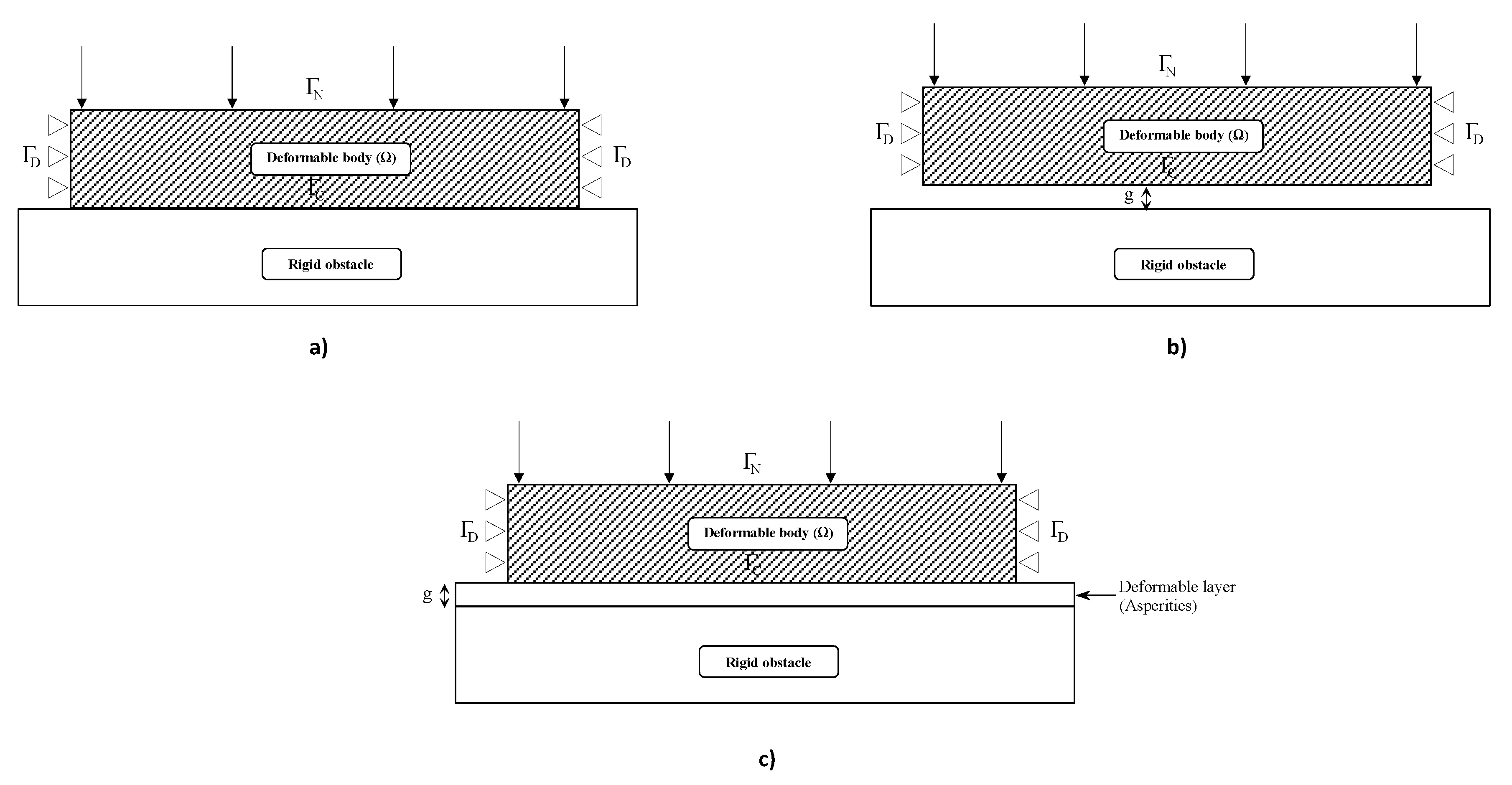
We start with the interface laws in the normal direction, the contact conditions, and consider two different physical settings. In the first one, the foundation is a rigid body and in the second one it is made of a rigid body covered by a layer of deformable material, which may be another material or just the surface asperities.

Contact conditions with a rigid body. First, we assume that the foundation is perfectly rigid, and there is no gap between the deformable body and the foundation, as shown in Figure 1a. Although there are no perfect rigid bodies, the conditions below turn out to be useful in many applied settings. A popular contact condition used both in engineering literature and mathematical publications is the Signorini contact condition, formulated as follows:

$$u_{\nu }\le 0,{\sigma }_{\nu }\le 0,{\sigma }_{\nu }{u}_{\nu }=0\mathrm{on}{\Gamma }_C.$$

(1)

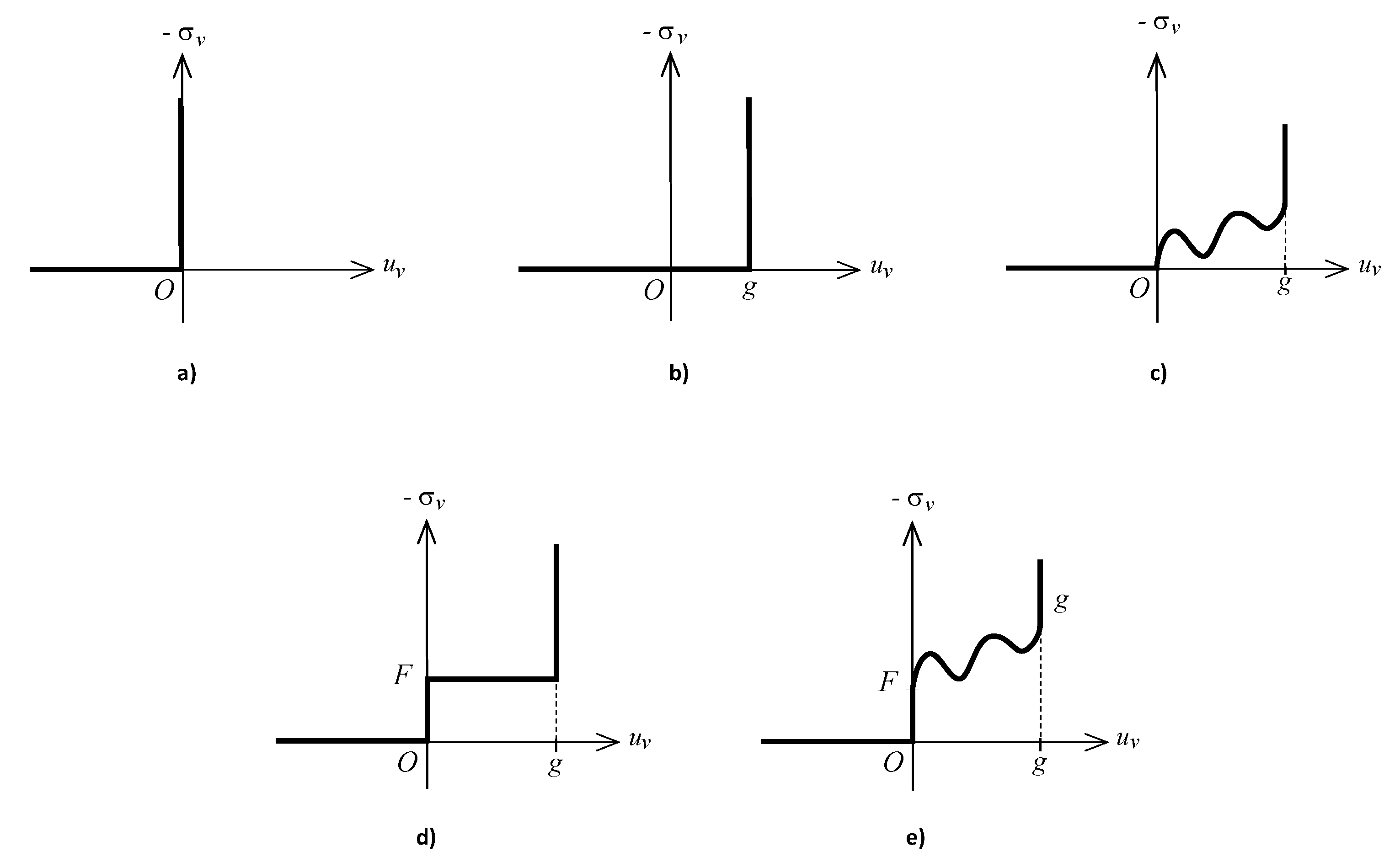
This condition was first introduced in [20] and then used in many papers, see e.g., Ref. [7] and the references therein. This condition doesn’t allow interpenetration. When $u_{\nu }<0$, there is separation between the body and the foundation and (1) implies that ${\sigma }_{\nu }=0$, i.e., the normal stress vanishes. When $u_{\nu }=0$, there is contact. Therefore, (1) implies that ${\sigma }_{\nu }\le 0$, i.e., the reaction of the foundation is towards the body. A graphic representation of the the Signorini condition (1) is provided in Figure 2a.

In the next case, we assume in addition that there is a gap $g>0$, in the reference configuration, between the body and the foundation, see Figure 1b. Then, the Signorini condition reads

$$u_{\nu }\le g,{\sigma }_{\nu }\le 0,{\sigma }_{\nu }(u_{\nu }-g)=0\mathrm{on}{\Gamma }_C.$$

(2)

The mechanical interpretations of (2) is very similar to the case $g=0$, and, graphically, it is depicted in Figure 2b.

We next consider more complex conditions.

Contact conditions with a rigid body covered by a deformable layer. Consider now the case when the foundation is made of a rigid body covered with a layer of deformable material of thickness $g>0$. This layer may be just the asperities or a softer material, as is shown is shown in Figure 1c. Then, since the rigid obstacle is impenetrable, we have

$$u_{\nu }\le g.$$

(3)

Moreover, using the principle of superposition, it follows that the normal stress has an additive decomposition of the form

$${\sigma }_{\nu }={\sigma }_{\nu }^D+{\sigma }_{\nu }^R,$$

(4)

in which ${\sigma }_{\nu }^D$ describes the reaction of the deformable layer and ${\sigma }_{\nu }^R$ describes the reaction of the rigid body.

Assume now that the deformable layer has an elastic behavior. Then, for the part ${\sigma }_{\nu }^D$ of the normal stress, we use the so-called normal compliance contact condition, which assigns a reactive normal pressure that depends on the interpenetration of the asperities on the body’s surface and those of the foundation. Therefore,

$$-{\sigma }_{\nu }^D=p\left(u_{\nu }\right)$$

(5)

where p is a nonnegative regular function that vanishes for a negative argument. Indeed, when $u_{\nu }<0$, there is no contact and the normal pressure vanishes. When $0\le u_{\nu }\le g$, there is contact and $u_{\nu }$ represents a measure of the interpenetration into the elastic layer. Then, condition (5) shows that the layer exerts on the body a pressure that depends on the penetration. In addition, when $u_{\nu }=g$, this layer is completely squeezed, and the normal pressure it exerts is $p\left(g\right)$. The normal compliance contact condition was first introduced in [21] and since then used in many publications, see e.g., Refs. [13,22,23,24] and the references therein. On the other hand, for the rigid part of the obstacle, we use the Signorini contact condition with a gap (2). Therefore,

$${\sigma }_{\nu }^R\le 0,{\sigma }_{\nu }^R(u_{\nu }-g)=0$$

(6)

and recall that $g>0$ represents the thickness of the deformable layer. We now gather conditions (3)–(6) and, in this way, we obtain the contact condition

$$\begin{array}{c}\hfill \left.u_{\nu }\le g,\begin{array}{cc}{\sigma }_{\nu }=0\hfill & \mathrm{if}{u}_{\nu }<0\hfill \\ -{\sigma }_{\nu }=p\left(u_{\nu }\right)\hfill & \mathrm{if}0\le u_{\nu }<g\hfill \\ -{\sigma }_{\nu }\ge p\left(g\right)\hfill & \mathrm{if}{u}_{\nu }=g\hfill \end{array}\right\}\mathrm{on}{\Gamma }_C.\end{array}$$

(7)

A graphic depiction of the contact condition (7) is provided in Figure 2c.

Next, we also consider the case when the deformable layer has a rigid-plastic behavior. In this case, in addition to (3), (4), and (6), we assume that

$$-F\le {\sigma }_{\nu }^D\le 0,{\sigma }_{\nu }^D=\left\{\begin{array}{c}0\mathrm{if}{u}_{\nu }<0,\hfill \\ -F\mathrm{if}{u}_{\nu }>0.\hfill \end{array}\right.$$

(8)

Here, F is a given positive traction threshold that may depend on the spatial variable x. Using (8), we have

$$\begin{array}{ccc}& & -F<{\sigma }_{\nu }^P\le 0⟹u_{\nu }\le 0,\hfill \\ & & {\sigma }_{\nu }^P=-F⟹u_{\nu }\ge 0.\hfill \end{array}$$

This shows that the layer does not allow penetration and, therefore, behaves as a rigid body, as far as the inequality $-F<{\sigma }_{\nu }^P\le 0$ holds. It allows penetration only when the threshold is reached, ${\sigma }_{\nu }^P=-F$ and, then, it offers no additional resistance, as surface plastic flow commences. Thus, conditions (8) model the situation when the deformable layer has a rigid-plastic behavior. Moreover, the function F could be interpreted as the yield limit. Gathering conditions (3), (4), (6), and (8) yields the contact condition

$$\begin{array}{c}\hfill u_{\nu }\le g,\left.\begin{array}{cc}{\sigma }_{\nu }=0\hfill & \mathrm{if}{u}_{\nu }<0\hfill \\ -F\le {\sigma }_{\nu }\le 0\hfill & \mathrm{if}{u}_{\nu }=0\hfill \\ {\sigma }_{\nu }=-F\hfill & \mathrm{if}0<u_{\nu }<g\hfill \\ {\sigma }_{\nu }\le -F\hfill & \mathrm{if}{u}_{\nu }=g\hfill \end{array}\right\}\mathrm{on}{\Gamma }_C.\end{array}$$

(9)

We may summarize this condition as follows:

(a)

If $u_{\nu }<0$, there is no contact and then (8) implies that ${\sigma }_{\nu }^D=0$, (5) implies that ${\sigma }_{\nu }^R=0$ and, therefore, equality (4) shows that ${\sigma }_{\nu }=0$. Thus, the contact traction vanishes, as expected.

(b)

If $u_{\nu }=0$, contact has just been established (or is about to be lost) and then (8) implies that $-F\le {\sigma }_{\nu }^D\le 0$, (5) implies that ${\sigma }_{\nu }^R=0$ and, therefore, equality (4) shows that $-F\le {\sigma }_{\nu }\le 0$. Thus, the layer behaves as a rigid surface.

(c)

If $0<u_{\nu }<g$, there is thus interpenetration into the layer, and then (8) implies that ${\sigma }_{\nu }^D=-F$, and (5) implies that ${\sigma }_{\nu }^R=0$ and, therefore, equality (4) shows that ${\sigma }_{\nu }=-F$. The layer is in the plastic flow regime.

(d)

If $u_{\nu }=g$, the layer is completely squashed, and then (8) implies that ${\sigma }_{\nu }^P=-F$, and (5) implies that ${\sigma }_{\nu }^R\le 0$ and, therefore, equality (4) shows that ${\sigma }_{\nu }\le -F$.

The contact condition (9) is depicted in Figure 2d. It was used in a number of papers, see, e.g., Ref. [9] and the references therein.

Finally, we consider the case when the deformable layer has a rigid-elastic behavior. In this case, in addition to (3), (4), and (6), we assume that

$$\begin{array}{c}\hfill \left.\begin{array}{cc}{\sigma }_{\nu }^D=0\hfill & \mathrm{if}{u}_{\nu }<0\hfill \\ -F\le {\sigma }_{\nu }\le 0\hfill & \mathrm{if}{u}_{\nu }=0\hfill \\ -{\sigma }_{\nu }^D=F+p\left(u_{\nu }\right)\hfill & \mathrm{if}{u}_{\nu }>0\hfill \end{array}\right\}.\end{array}$$

(10)

Condition (10) represents a combination of conditions (5) and (8) in which F is a positive function and p is the normal compliance function; it is positive when the argument is positive and vanishes for a negative argument. Arguments similar to those above show that now the behavior of the deformable layer is rigid-elastic. Here, F could be interpreted as the yield limit of the layer, while the normal compliance function p describes its elastic properties. We now gather (3), (4), (6), and (10) to obtain the following contact condition:

$$\begin{array}{c}\hfill \left.u_{\nu }\le g,\begin{array}{cc}{\sigma }_{\nu }=0\hfill & \mathrm{if}{u}_{\nu }<0\hfill \\ -F\le {\sigma }_{\nu }\le 0\hfill & \mathrm{if}{u}_{\nu }=0\hfill \\ -{\sigma }_{\nu }=F+p\left(u_{\nu }\right)\hfill & \mathrm{if}0<u_{\nu }<g\hfill \\ -{\sigma }_{\nu }\ge F+p\left(u_{\nu }\right)\hfill & \mathrm{if}{u}_{\nu }=g\hfill \end{array}\right\}\mathrm{on}{\Gamma }_C.\end{array}$$

(11)

This condition is depicted in Figure 2e.

Comments on the contact conditions (1), (2), (7), (9), and (11). First, these conditions are expressed in terms of unilateral constraints and are governed by the data $g,p$, and F. Moreover, all of them are described by multivalued relations between the normal displacement and the compressive normal stress, see Figure 2. In addition, there exists a hierarchy among these contact conditions as follows:

(a)

Condition (9) can be obtained from condition (11) when the normal compliance function p vanishes, i.e., $p\equiv 0$.

(b)

Condition (7) is obtained from condition (11) when the yield limit F vanishes, i.e., $F=0$.

(c)

Condition (2) can be recovered from condition (9), when $p\equiv 0$, from condition (7) when $F=0$ and from condition (11) when $p\equiv 0$ and $F=0$.

(d)

The Signorini contact condition (1) is obtained from conditions (2), (7), (9), and (11) when $g=0$.

We conclude that, among the above conditions, condition (11) is the most general one. For this reason, it will play a special role in the next two sections.

Coulomb’s law of dry friction. We end this section with the conditions in the tangential directions, also called frictional conditions or friction laws. The simplest one is the so-called frictionless condition in which the tangential part of the stress vanishes. This is an idealization of the process, since even completely lubricated surfaces generate shear resistance to tangential motion. For this reason, we assume in what follows that the tangential traction ${\mathbf{\sigma }}_{\tau }$ does not vanish on the contact surface, i.e., the contact is with friction.

Frictional contact between solid surfaces without lubrication is usually modeled with a number of variants of the Coulomb law of dry friction. The classical static version of this law, commonly used in frictional contact problems describing the equilibrium states of elastic bodies, is formulated as follows:

$$\parallel {\mathbf{\sigma }}_{\tau }\parallel \le \mu |{\sigma }_{\nu }|,{\mathbf{\sigma }}_{\tau }=-\mu \left|{\sigma }_{\nu }\right|\frac{{\mathit{u}}_{\tau }}{\parallel {\mathit{u}}_{\tau }\parallel }if{\mathit{u}}_{\tau }\ne \mathbf{0}\mathrm{on}{\Gamma }_C.$$

(12)

Here, $\mu >0$ is the coefficient of friction and $\parallel {\mathbf{\sigma }}_{\tau }\parallel$ represents the norm of the friction force. The friction law (12) was intensively studied in the literature; see, for instance, the references in [7]. It shows that, during the contact process, the magnitude of the friction force is bounded by the positive function $\mu |{\sigma }_{\nu }|$, the friction bound. This is the maximal strength that friction resistance can provide, and above it the surfaces undergo a relative motion. It indicates that the points on the contact surface where the inequality $\parallel {\mathbf{\sigma }}_{\tau }\parallel <\mu |{\sigma }_{\nu }|$ holds are in the stick state since there ${\mathit{u}}_{\tau }=\mathbf{0}$. The points of the contact surface where ${\mathit{u}}_{\tau }\ne \mathbf{0}$ are in the slip state. There, the friction force ${\mathbf{\sigma }}_{\tau }$ is opposite to the slip ${\mathit{u}}_{\tau }$ and, moreover, its magnitude equals the magnitude of the friction bound since, in this case, (12) implies that $\parallel {\mathbf{\sigma }}_{\tau }\parallel =\mu |{\sigma }_{\nu }|$.

We note here that “friction force” is not a force in the usual sense, since friction is only resistance to motion and cannot initiate motion, unlike a “real” force. Although we use the term friction force, “frictional resistance force” is the more accurate term in physics, since it just opposes motion.

We now combine Coulomb’s law (12) with each one of the contact conditions (1), (2), (7), (9), or (11), and obtain a specific boundary condition. We note that, when there is separation between the surfaces (i.e., when $u_{\nu }<0$ in the case of conditions (1), (7), (9), or (11), and $u_{\nu }<g$ in the case of condition (2)), then ${\sigma }_{\nu }=0$ and, therefore, the friction bound in (12) vanishes. This, in turn, implies that ${\mathbf{\sigma }}_{\tau }=\mathbf{0}$, i.e., the friction resistance force vanishes too. This property is realistic from a physical point of view and expresses the compatibility between the contact conditions with unilateral constraints considered above and the Coulomb law of dry friction.

In mathematical publications, and for mathematical reasons mentioned shortly, the classical Coulomb’s law of dry friction (12) needs to be modified, and is very often used in its regularized version

$$\parallel {\mathbf{\sigma }}_{\tau }\parallel \le \mu |\mathcal{R}{\sigma }_{\nu }|,{\mathbf{\sigma }}_{\tau }=-\mu \left|\mathcal{R}{\sigma }_{\nu }\right|\frac{{\mathit{u}}_{\tau }}{\parallel {\mathit{u}}_{\tau }\parallel }\mathrm{if}{\mathit{u}}_{\tau }\ne \mathbf{0}\mathrm{on}{\Gamma }_C.$$

(13)

Here, $\mathcal{R}$ is a continuous regularizing operator that may be considered as the average of the normal stress over a small patch around the contact point. The inclusion of this operator can be traced to [25,26]. As explained in [25], there seems to be some physical justification in considering the normal stress in the friction condition (13) as averaged over a small surface area which contains many asperities, since the physical contact point usually contains many asperities, and the contact surface is rarely smooth. However, the main motivation for such a choice is mathematical, to avoid otherwise insurmountable difficulties. Indeed, in the weak formulation, the regularity of the stress $\mathbf{\sigma }$ does not allow a meaningful definition of the absolute value of the normal stress ${\sigma }_{\nu }$ on the boundary. To overcome this difficulty, the operator $\mathcal{R}$ has been introduced in [26]. As an example of such an operator, one may use the convolution of $\mathbf{\sigma }$ with an infinitely differentiable function that has support in a small area that includes the point where the condition is applied.

The constitutive law of an elastic material is such that $\mathbf{\sigma }$ depends explicitly on u, and we may write it as $\mathbf{\sigma }=\mathbf{\sigma }\left(\mathit{u}\right)$, which, in turn, implies that ${\sigma }_{\nu }={\sigma }_{\nu }\left(\mathit{u}\right)$. Therefore, denoting by R the regularizing operator defined by

$$R\mathit{u}=\mathcal{R}{\sigma }_{\nu }\left(\mathit{u}\right),$$

in the case of elastic materials, we can write the regularized friction law (13) as follows:

$$\parallel {\mathbf{\sigma }}_{\tau }\parallel \le \mu \left|R\mathit{u}\right|,{\mathbf{\sigma }}_{\tau }=-\mu \left|R\mathit{u}\right|\frac{{\mathit{u}}_{\tau }}{\parallel {\mathit{u}}_{\tau }\parallel }\mathrm{if}{\mathit{u}}_{\tau }\ne \mathbf{0}\mathrm{on}{\Gamma }_C.$$

(14)

Details on the regularized friction law (14) can be found in [7] and, therefore, we skip them here. We just mention that in this paper we deal with contact problems for linearly elastic materials and, therefore, we use the regularized version (14) of Coulomb’s law of dry friction. The properties of the regularizing operator R will be described in the next section.

3. Main Problem and Variational Formulation

This section presents the physical setting of the contact problem we are interested in, lists the assumption on the problem data, and derives its variational formulation.

Assume that a deformable solid body occupies, in the reference configuration, an open, bounded, and connected set $\Omega \subset {\mathbb{R}}^d$ ($d=2,3$). The boundary $\Gamma =\partial \Omega$ is composed of three relatively closed sets ${\overline{\Gamma }}_D$, ${\overline{\Gamma }}_N$ and ${\overline{\Gamma }}_C$, such that the relatively open sets ${\Gamma }_D$, ${\Gamma }_N$, and ${\Gamma }_C$ are mutually disjoint and, moreover, the measure of ${\Gamma }_D$ is positive. The body is clamped on ${\Gamma }_D$. Tractions of surface density ${\mathit{f}}_N$ act on ${\Gamma }_N$ and, moreover, body forces of density (per unit volume) ${\mathit{f}}_0$ act in $\Omega$. The body can come into contact on ${\Gamma }_C$ with another solid, which is called an “obstacle” or “foundation”, as shown in Figure 1. Our interest is in the static mechanical equilibrium; the body is assumed to be linearly elastic; and the main interest is in what happens on the contacting surface.

We use bold face letters for vectors and tensors; the outward unit normal on $\Gamma$ is denoted by $\mathit{\nu }$; the spatial variable is denoted by x and, in order to simplify the notation, we do not indicate explicitly the dependence of the various functions on x.

We denote by ${\mathbb{S}}^d$ the space of second order symmetric tensors on ${\mathbb{R}}^d$ and $\mathit{u}:\Omega \to {\mathbb{R}}^d$ and $\mathbf{\sigma }:\Omega \to {\mathbb{S}}^d$ represent the displacement and the stress fields, respectively. The mathematical model that describes the equilibrium of the elastic body, under the previous mechanical assumptions, consists of the following equations:

$$\begin{array}{ccc}\hfill \mathbf{\sigma }=\mathcal{E}\mathbf{\epsilon }\left(\mathit{u}\right)& \mathrm{in}& \Omega ,\hfill \end{array}$$

(15)

$$\begin{array}{ccc}\hfill \mathrm{Div}\mathbf{\sigma }+{\mathit{f}}_0=\mathbf{0}& \mathrm{in}& \Omega .\hfill \end{array}$$

(16)

The elastic constitutive law is given in (15) in which $\mathcal{E}$ is the elasticity tensor, and $\mathbf{\epsilon }\left(\mathit{u}\right)$ denotes the linearized strain field. The equilibrium Equation (16) describes the static process that is assumed here. Next, the displacement–traction boundary conditions associated with this physical settings are

$$\begin{array}{ccc}\hfill \mathit{u}=\mathbf{0}& \mathrm{on}& {\Gamma }_D,\hfill \end{array}$$

(17)

$$\begin{array}{ccc}\hfill \mathbf{\sigma }\mathbf{\nu }={\mathit{f}}_N& \mathrm{on}& {\Gamma }_N.\hfill \end{array}$$

(18)

To complete the model, we add the friction law (14) and one of the contact conditions introduced in Section 2. We recall that condition (11) is the most general one and, therefore, we start by using this contact condition. Since it is governed by the data g, p, F, we denote in what follows by ${\mathcal{P}}_{gpF}$ the resulting mathematical model. To conclude, the main problem we consider can be stated as follows.

Problem 1.

${\mathcal{P}}_{gpF}$. Find a displacement field $\mathit{u}=\mathit{u}(g,p,F):\Omega \to {\mathbb{R}}^d$ and a stress field $\mathbf{\sigma }=\mathbf{\sigma }(g,p,F):\Omega \to {\mathbb{S}}^d$ that satisfy (15)–(18), (11) and (14).

In the variational analysis of this problem, we denote by “·”, $\parallel ·\parallel$ and 0 the inner product, the Euclidean norm, and the zero element of the spaces ${\mathbb{R}}^d$ and ${\mathbb{S}}^d$, respectively. We use the standard notation for the Sobolev and Lebesgue spaces associated with $\Omega \subset {\mathbb{R}}^d$ and $\Gamma$ and, for an element $\mathit{v}\in H^1{(\Omega )}^d$, we usually write v for the trace $\gamma \mathit{v}\in L^2{(\Gamma )}^d$ of v on $\Gamma$. Moreover, we denote by $v_{\nu }$ and ${\mathit{v}}_{\tau }$ the normal and tangential components of v on the boundary, given by $v_{\nu }=\mathit{v}·\mathbf{\nu }$ and ${\mathit{v}}_{\tau }=\mathit{v}-v_{\nu }\mathbf{\nu }$, respectively. We also use the spaces

$$\begin{array}{ccc}& & V=\{\mathit{v}=\left(v_i\right)\in H^1{(\Omega )}^d:\mathit{v}=\mathbf{0}\mathrm{on}{\Gamma }_D\},\hfill \\ & & Q=\{\mathbf{\sigma }=\left({\sigma }_{ij}\right):{\sigma }_{ij}={\sigma }_{ji}\in L^2(\Omega ),i,j=1,\cdots ,d\},\hfill \end{array}$$

which are real Hilbert spaces endowed with the canonical inner products

$${(\mathit{u},\mathit{v})}_V={\int }_{\Omega }\mathbf{\epsilon }\left(\mathit{u}\right)·\mathbf{\epsilon }\left(\mathit{v}\right)dx,{(\mathbf{\sigma },\mathbf{\tau })}_Q={\int }_{\Omega }\mathbf{\sigma }·\mathbf{\tau }dx.$$

(19)

Recall that, in (19) and (16), $\mathbf{\epsilon }$ and $\mathrm{Div}$ represent the deformation and the divergence operators, respectively, i.e.,

$$\mathbf{\epsilon }\left(\mathit{u}\right)=\left({\epsilon }_{ij}\left(\mathit{u}\right)\right),{\epsilon }_{ij}\left(\mathit{u}\right)=\frac{1}{2}(u_{i,j}+u_{j,i}),\mathrm{Div}\mathbf{\sigma }=\left({\sigma }_{ij,j}\right).$$

Here and below, an index that follows a comma denotes the partial derivative with respect to the corresponding component of x, i.e., $u_{i,j}=\partial u_i/\partial x_j$, and the summation convention over a repeated index is used. The associated norms on these spaces are denoted by ${\parallel ·\parallel }_V$ and ${\parallel ·\parallel }_Q$, respectively. We use ${}^{\prime \prime }\to {}^{\prime \prime }$ and ${}^{\prime \prime }\rightharpoonup {}^{\prime \prime }$ to denote the strong and the weak convergence on V and ${\mathbf{0}}_V$ for the zero element in V. Moreover, it follows from the Sobolev trace arguments that there exists a constant $c_0>0$ such that

$$\begin{array}{ccc}& & {\parallel \mathit{v}\parallel }_{L^2{\left({\Gamma }_C\right)}^d}\le c_0{\parallel \mathit{v}\parallel }_V,\forall \mathit{v}\in V.\hfill \end{array}$$

(20)

Finally, we recall that, for a regular stress function $\mathbf{\sigma }$, the following Green’s formula holds:

$${\int }_{\Omega }\mathbf{\sigma }·\mathbf{\epsilon }\left(\mathit{v}\right)dx+{\int }_{\Omega }\mathrm{Div}\mathbf{\sigma }·\mathit{v}dx={\int }_{\Gamma }\mathbf{\sigma }\mathbf{\nu }·\mathit{v}dS,\forall \mathit{v}\in H^1{(\Omega )}^d.$$

(21)

We now list the assumption on the data of the contact problem ${\mathcal{P}}_{gpF}$. The elasticity tensor $\mathcal{E}$ is symmetric and positively definite, i.e., it satisfies the conditions

$$\left\{\begin{array}{c}\left(\mathrm{a}\right)\mathcal{E}=\left({\mathcal{E}}_{ijkl}\right):\Omega \times {\mathbb{S}}^d\to {\mathbb{S}}^d,\hfill \\ \left(\mathrm{b}\right){\mathcal{E}}_{ijkl}={\mathcal{E}}_{klij}={\mathcal{E}}_{jikl}\in L^{\infty }(\Omega ),1\le i,j,k,l\le d,\hfill \\ \left(\mathrm{c}\right)\mathrm{There}\mathrm{exists}{m}_{\mathcal{E}}>0\mathrm{such}\mathrm{that}\hfill \\ \mathcal{E}\mathbf{\tau }·\mathbf{\tau }\ge m_{\mathcal{E}}{\parallel \mathbf{\tau }\parallel }^2\forall \mathbf{\tau }\in {\mathbb{S}}^d,\mathrm{a}.\mathrm{e}.\mathrm{in}\Omega .\hfill \end{array}\right.$$

(22)

The regularization operator R is Lipschitz continuous, i.e.,

$$\left\{\begin{array}{c}R:V\to L^2\left({\Gamma }_C\right)\mathrm{and} \mathrm{there} \mathrm{exists}{L}_R>0\mathrm{such}\mathrm{that}\hfill \\ {\parallel R\mathit{u}-R\mathit{v}\parallel }_{L^2\left({\Gamma }_C\right)}\le L_R{\parallel \mathit{u}-\mathit{v}\parallel }_V\mathrm{for} \mathrm{all}\mathit{u},\mathit{v}\in V.\hfill \end{array}\right.$$

(23)

We also assume that the densities of the body forces and surface tractions and the thickness of the deformable layer are such that

$$\begin{array}{ccc}& & {\mathit{f}}_0\in L^2{(\Omega )}^d.\hfill \end{array}$$

(24)

$$\begin{array}{ccc}& & {\mathit{f}}_N\in L^2{\left({\Gamma }_N\right)}^d.\hfill \end{array}$$

(25)

$$\begin{array}{ccc}& & g\ge 0.\hfill \end{array}$$

(26)

Moreover, the normal compliance function p, the yield limit F, and the coefficient of friction $\mu$ satisfy the following conditions:

$$\left\{\begin{array}{c}p:{\Gamma }_C\times \mathbb{R}\to {\mathbb{R}}_{+}\mathrm{and}\hfill \\ \left(\mathrm{a}\right)\mathrm{there}\mathrm{exists}{L}_p>0\mathrm{such}\mathrm{that}\hfill \\ |p(\mathit{x},r_1)-p(\mathit{x},r_2)|\le L_p|r_1-r_2|\hfill \\ \mathrm{for} \mathrm{all}{r}_1,r_2\in \mathbb{R},\mathrm{a}.\mathrm{e}.\mathit{x}\in {\Gamma }_C,\hfill \\ \left(\mathrm{b}\right)p(·,r)\mathrm{is}\mathrm{measurable}\mathrm{on}{\Gamma }_C\mathrm{for}\mathrm{all}r\in \mathbb{R},\hfill \\ \left(\mathrm{c}\right)p(\mathit{x},r)=0\mathrm{if} \mathrm{and} \mathrm{only} \mathrm{if}r\le 0,\mathrm{a}.\mathrm{e}.\mathit{x}\in {\Gamma }_C.\hfill \end{array}\right.$$

(27)

$$\begin{array}{ccc}& & F\in L^2\left({\Gamma }_C\right),F\left(\mathit{x}\right)\ge 0\mathrm{a}.\mathrm{e}.\mathit{x}\in {\Gamma }_C.\hfill \end{array}$$

(28)

$$\begin{array}{ccc}& & \mu \in L^{\infty }\left({\Gamma }_C\right),\mu \left(\mathit{x}\right)\ge 0\mathrm{a}.\mathrm{e}.\mathit{x}\in {\Gamma }_C.\hfill \end{array}$$

(29)

Finally, we assume that the following smallness condition holds:

$$c_0^2{L}_p+c_0{L}_R{\parallel \mu \parallel }_{L^{\infty }\left({\Gamma }_C\right)}<m_{\mathcal{E}},$$

(30)

where $c_0$, $L_R$, $L_p$, and $m_{\mathcal{E}}$ are the positive constants in (20), (23), (27), and (22), respectively.

We turn to construct a variational inequality formulation of the problem. To that end, we consider the set $K_g\subset V$, the form $a:V\times V\to \mathbb{R}$, the function $j_{pF}:V\times V\to \mathbb{R}$ and the element $\mathit{f}\in V$ defined by

$$\begin{array}{ccc}& & K_g=\{\mathit{v}\in V:v_{\nu }\le g\mathrm{a}.\mathrm{e}.\mathrm{on}{\Gamma }_C\},\hfill \end{array}$$

(31)

$$\begin{array}{ccc}& & a(\mathit{u},\mathit{v})={\int }_{\Omega }\mathcal{E}\mathbf{\epsilon }\left(\mathit{u}\right)·\mathbf{\epsilon }\left(\mathit{v}\right)dx,\forall \mathit{u},\mathit{v}\in V,\hfill \\ & & j_{pF}(\mathit{u},\mathit{v})={\int }_{{\Gamma }_C}p\left(u_{\nu }\right)v_{\nu }dS+{\int }_{{\Gamma }_C}F{v}_{\nu }^{+}dS+{\int }_{{\Gamma }_C}\mu \left|R\mathit{u}\right|\parallel {\mathit{v}}_{\tau }\parallel dS,\forall \mathit{u},\mathit{v}\in V,\hfill \end{array}$$

(32)

$$\begin{array}{ccc}& & {(\mathit{f},\mathit{v})}_V={\int }_{\Omega }{\mathit{f}}_0·\mathit{v}dx+{\int }_{{\Gamma }_N}{\mathit{f}}_N·\mathit{v}dS,\forall \mathit{v}\in V,\hfill \end{array}$$

(33)

where, here and below, $r^{+}$ represents the positive part of r, which is $r^{+}=max\{r,0\}$.

Next, standard arguments based on the Green formula (21) show that, if $(\mathit{u},\mathbf{\sigma })$ is a smooth solution of Problem ${\mathcal{P}}_{gpF}$ and $v\in K_g$, then

$$\begin{array}{ccc}& & {\int }_{\Omega }\mathcal{E}\mathbf{\epsilon }\left(\mathit{u}\right)·(\mathbf{\epsilon }\left(\mathit{v}\right)-\mathbf{\epsilon }\left(\mathit{u}\right))dx={\int }_{\Omega }{\mathit{f}}_0·(\mathit{v}-\mathit{u})dx+{\int }_{{\Gamma }_N}{\mathit{f}}_N·(\mathit{v}-\mathit{u})dS\hfill \\ & & +{\int }_{{\Gamma }_C}{\sigma }_{\nu }(v_{\nu }-u_{\nu })dS+{\int }_{{\Gamma }_C}{\mathbf{\sigma }}_{\tau }·({\mathit{v}}_{\tau }-{\mathit{u}}_{\tau })dS.\hfill \end{array}$$

(34)

To deal with the third term on the right-hand side, we rewrite it as

$$\begin{array}{ccc}& & {\sigma }_{\nu }(v_{\nu }-u_{\nu })=({\sigma }_{\nu }+F+p\left(u_{\nu }\right))(v_{\nu }-g)+({\sigma }_{\nu }+F+p\left(u_{\nu }\right))(g-u_{\nu })\hfill \\ & & +F(u_{\nu }-v_{\nu })+p\left(u_{\nu }\right)(u_{\nu }-v_{\nu }),\hfill \end{array}$$

and, using the boundary conditions (11), we deduce that

$$\begin{array}{ccc}& & {\int }_{{\Gamma }_C}{\sigma }_{\nu }(v_{\nu }-u_{\nu })dS\ge {\int }_{{\Gamma }_C}F(u_{\nu }^{+}-v_{\nu }^{+})dS+{\int }_{{\Gamma }_C}p\left(u_{\nu }\right)(u_{\nu }-v_{\nu })dS.\hfill \end{array}$$

(35)

Moreover, using the friction law (14), we find that

$$\begin{array}{ccc}& & {\int }_{{\Gamma }_C}{\mathbf{\sigma }}_{\tau }·({\mathit{v}}_{\tau }-{\mathit{u}}_{\tau })dS\ge {\int }_{{\Gamma }_C}\mu \left|R\mathit{u}\right|(\parallel {\mathit{u}}_{\tau }\parallel -\parallel {\mathit{v}}_{\tau }\parallel )dS.\hfill \end{array}$$

(36)

We now combine (34) with inequalities (35) and (36) and obtain

$$\begin{array}{ccc}& & {\int }_{\Omega }\mathcal{E}\mathbf{\epsilon }\left(\mathit{u}\right)·(\mathbf{\epsilon }\left(\mathit{v}\right)-\mathbf{\epsilon }\left(\mathit{u}\right))dx+{\int }_{{\Gamma }_C}F(v_{\nu }^{+}-u_{\nu }^{+})dS+{\int }_{{\Gamma }_C}p\left(u_{\nu }\right)(v_{\nu }-u_{\nu })dS\hfill \\ & & +{\int }_{{\Gamma }_C}\mu \left|R\mathit{u}\right|(\parallel {\mathit{v}}_{\tau }\parallel -\parallel {\mathit{u}}_{\tau }\parallel )dS\ge {\int }_{\Omega }{\mathit{f}}_0·(\mathit{v}-\mathit{u})dx+{\int }_{{\Gamma }_N}{\mathit{f}}_2·(\mathit{v}-\mathit{u})dS.\hfill \end{array}$$

(37)

Finally, we use inequality (37), the notations (32) and (33) and the fact that $\mathit{u}\in K_g$ to obtain the following variational formulation of Problem ${\mathcal{P}}_{gpF}$, in terms of the displacements.

Problem 2.

${\mathcal{P}}_{gpF}^V$. Find a displacement field $\mathit{u}=\mathit{u}(g,p,F)$ such that

$$\begin{array}{ccc}& & \mathit{u}\in K_g,a(\mathit{u},\mathit{v}-\mathit{u})+j_{pF}(\mathit{u},\mathit{v})-j_{pF}(\mathit{u},\mathit{u})\ge {(\mathit{f},\mathit{v}-\mathit{u})}_V,\forall \mathit{v}\in K_g.\hfill \end{array}$$

(38)

A function $\mathit{u}=\mathit{u}(g,p,F)$ which satisfies inequality (38) is called a weak solution of the contact problem ${\mathcal{P}}_{gpF}$. Once the existence of a weak solution is found, the stress function can be obtained by using the elastic constitutive law (15).

4. Tykhonov Well-Posedness

In this section, we study the Tykhonov well-posedness of Problem ${\mathcal{P}}_{gpF}^V$ and, to this end, we start by recalling some of the necessary abstract setting and concepts introduced in [15].

Consider an abstract mathematical object $\mathcal{P}$, called a generic ”problem,” that is associated with a metric space $(X,\tilde{d})$. Problem $\mathcal{P}$ could be an equation, or a problem of minimization, a fixed point, an inclusion, or an inequality. We associate with Problem $\mathcal{P}$ the concept of “solution”, which depends on the context. We also denote by ${\mathcal{S}}_{\mathcal{P}}\subset X$ the set of solutions to Problem $\mathcal{P}$. Problem $\mathcal{P}$ has a unique solution iff ${\mathcal{S}}_{\mathcal{P}}$ has a unique element, i.e., ${\mathcal{S}}_{\mathcal{P}}$ is a singleton. For a nonempty set B, we denote by $\mathcal{S}\left(B\right)$ the set of sequences whose elements belong to B, and $2^B$ is the set of all nonempty subsets of B. The concept of well-posedness for Problem $\mathcal{P}$ is related to the so-called Tykhonov triple, defined as follows.

Definition 1.

A Tykhonov triple is a mathematical object of the form $\mathcal{T}=(I,\Theta ,\mathcal{C})$, where I is a given nonempty set, $\Theta :I\to 2^X$ and $\mathcal{C}$ is a nonempty subset of the set $\mathcal{S}\left(I\right)$.

Below, we refer to I as the set of parameters; the family of sets ${\{\Theta \left(\theta \right)\}}_{\theta \in I}$ represents the family of approximating sets; finally, $\mathcal{C}$ defines the criterion of convergence.

Definition 2.

Given a Tykhonov triple $\mathcal{T}=(I,\Theta ,\mathcal{C})$, a sequence $\left\{u_n\right\}\in \mathcal{S}\left(X\right)$ is called an approximating sequence if there exists a sequence $\left\{{\theta }_n\right\}\in \mathcal{C}$ such that $u_n\in \Theta \left({\theta }_n\right)$ for each $n\in \mathbb{N}$.

Definition 3.

Given a Tykhonov triple $\mathcal{T}=(I,\Theta ,\mathcal{C})$, Problem $\mathcal{P}$ is said to be well-posed in the sense of Tykhonov if it has a unique solution, and every approximating sequence converges in X to this solution.

We remark that approximating sequences always exist since, by assumption, $\mathcal{C}\ne \varnothing$ and, moreover, for any sequence $\left\{{\theta }_n\right\}\in \mathcal{C}$ and any $n\in \mathbb{N}$, the set $\Theta \left({\theta }_n\right)$ is not empty. In addition, the concept of approximating sequence depends on the Tykhonov triple $\mathcal{T}$ and, for this reason, we use the terminology “$\mathcal{T}$-approximating sequence”. As a consequence, the concept of well-posedness depends on the Tykhonov triple $\mathcal{T}$ and, therefore, we refer to it as “well-posedness with respect to $\mathcal{T}$” or “$\mathcal{T}$-well-posedness,” for short.

We turn now on the well-posedness of Problem ${\mathcal{P}}_{gpF}^V$ and, to this end, we consider the Tykhonov triple $\mathcal{T}=(I,\Theta ,\mathcal{C})$, defined as follows:

$$\begin{array}{ccc}& & I=\{\theta =(\tilde{g},\epsilon )\in {\mathbb{R}}^2:g\ge 0,\epsilon \ge 0\},\hfill \end{array}$$

(39)

$$\begin{array}{ccc}& & \Theta \left(\theta \right)=\{\mathit{u}\in K_{\tilde{g}}:a(\mathit{u},\mathit{v}-\mathit{u})+j_{pF}(\mathit{u},\mathit{v})-j_{pF}(\mathit{u},\mathit{u})\hfill \\ & & {+\epsilon \parallel \mathit{v}-\mathit{u}\parallel }_V\ge {(\mathit{f},\mathit{v}-\mathit{u})}_V\forall \mathit{v}\in K_{\tilde{g}}\}\mathrm{for}\theta =(\tilde{g},\epsilon )\in I,\hfill \end{array}$$

(40)

$$\begin{array}{ccc}& & \mathcal{C}=\{\left\{{\theta }_n\right\}\subset \mathcal{S}\left(I\right):{\theta }_n=(g_n,{\epsilon }_n)\forall n\in \mathbb{N},:g_n\to g,{\epsilon }_n\to 0\}.\hfill \end{array}$$

(41)

Here, $\tilde{g}$ represents a potential thickness and the set $K_{\tilde{g}}$ is defined by (31), replacing g with $\tilde{g}$. We next note that, for mathematical reasons, we introduce a positive parameter $\epsilon$ in the definition of the Tykhonov triple (39)–(41). Convenient choices of this parameter allow us to obtain various convergence results to the solution of the variational inequality (38), as we show in Section 5.

Our main result in this section is the following:

Theorem 1.

Assume that (22)–(30) holds. Then, Problem ${\mathcal{P}}_{gpF}^V$ is well-posed with respect to the Tykhonov triple (39)–(41).

The $\mathcal{T}$-well-posedness of Problem ${\mathcal{P}}_{gpF}^V$ can be established by using the general results on the well-posedness of variational-hemivariational inequalities in [27]. Nevertheless, the statement of the results there requires additional definitions and preliminaries and, therefore, for the convenience of the reader, we present here a direct proof of Theorem 1, which is structured in four steps, as follows.

Proof. 

(i) Existence of a unique solution of Problem ${\mathcal{P}}_{gpF}^V$. First, we remark that $K_g$, defined by (31), is a closed, nonempty, and convex set in V. Next, assumptions (22) on the elasticity tensor show that the bilinear form $a:V\times V\to \mathbb{R}$, defined by (32), is symmetric, continuous, and coercive. More precisely, it satisfies the inequality

$$a(\mathit{v},\mathit{v})\ge m_{\mathcal{E}}{\parallel \mathit{v}\parallel }_V^2,\forall \mathit{v}\in V.$$

(42)

In addition, using the assumptions (23), (27)–(29), it follows that the functional $j_{pF}(\mathit{u},·):V\to \mathbb{R}$ is convex and continuous. Then, the inequalities (20) and (23) imply that

$$\begin{array}{ccc}& & j_{pF}({\mathit{u}}_1,{\mathit{v}}_2)-j_{pF}({\mathit{u}}_1,{\mathit{v}}_1)+j_{pF}({\mathit{u}}_2,{\mathit{v}}_1)-j_{pF}({\mathit{u}}_1,{\mathit{v}}_2)\hfill \\ & & \le (c_0^2{L}_p+c_0{L}_R{\parallel \mu \parallel }_{L^{\infty }\left({\Gamma }_C\right)})\parallel {\mathit{u}}_1-{\mathit{u}}_2{\parallel }_V{\parallel {\mathit{v}}_1-{\mathit{v}}_2\parallel }_V,\forall {\mathit{u}}_1,{\mathit{u}}_2,{\mathit{v}}_1,{\mathit{v}}_2\in V.\hfill \end{array}$$

(43)

Inequalities (42) and (43) combined with the smallness assumption (30) allow us to use Theorem 3.7 in [28] to deduce the unique solvability of Problem ${\mathcal{P}}_{gpF}^V$.

(ii) Weak convergence of approximating sequences. Assume that $\left\{{\mathit{u}}_n\right\}$ is a $\mathcal{T}$-approximating sequence. Then, using Definition 2, we deduce that there exists a sequence $\left\{{\theta }_n\right\}\in \mathcal{C}$ such that ${\mathit{u}}_n\in \Theta \left({\theta }_n\right)$ for each $n\in \mathbb{N}$. Therefore, definitions (40), (41), and (31) imply that

$$\begin{array}{ccc}& & {\mathit{u}}_n\in K_{g_n},a({\mathit{u}}_n,\mathit{v}-{\mathit{u}}_n)+j_{pF}({\mathit{u}}_n,\mathit{v})-j_{pF}({\mathit{u}}_n,{\mathit{u}}_n)\hfill \\ & & +{\epsilon }_n{\parallel \mathit{v}-{\mathit{u}}_n\parallel }_V\ge {(\mathit{f},\mathit{v}-{\mathit{u}}_n)}_V\forall \mathit{v}\in K_{g_n},\hfill \end{array}$$

(44)

for each $n\in \mathbb{N}$, where

$$\begin{array}{ccc}& & K_{g_n}=\{\mathit{v}\in V:v_{\nu }\le g_n\mathrm{a}.\mathrm{e}.\mathrm{on}{\Gamma }_C\},\hfill \end{array}$$

(45)

and, moreover,

$$g_n\to g,$$

(46)

$${\epsilon }_n\to 0$$

(47)

as $n\to \infty$.

Let $n\in \mathbb{N}$ be fixed. We choose $v={\mathbf{0}}_V$ in (44) and, since $j({\mathit{u}}_n,{\mathbf{0}}_V)=0$, $j({\mathit{u}}_n,{\mathit{u}}_n)\ge 0$, we find that

$$a({\mathit{u}}_n,{\mathit{u}}_n)\le {\epsilon }_n{\parallel {\mathit{u}}_n\parallel }_V+{(\mathit{f},{\mathit{u}}_n)}_V.$$

Next, inequality (42) implies that

$$\parallel {\mathit{u}}_n{\parallel }_V\le \frac{1}{m_{\mathcal{E}}}({\epsilon }_n+{\parallel \mathit{f}\parallel }_V),$$

and, using (47), we obtain that the sequence $\left\{{\mathit{u}}_n\right\}$ is bounded in V. This, in turn, implies that there exists an element $\tilde{\mathit{u}}\in V$ and a subsequence of $\left\{{\mathit{u}}_n\right\}$, still denoted by $\left\{{\mathit{u}}_n\right\}$, such that

$${\mathit{u}}_n\rightharpoonup \tilde{\mathit{u}}\mathrm{in}V.$$

(48)

It follows that ${\mathit{u}}_n\to \tilde{\mathit{u}}$ a.e. on ${\Gamma }_C$ and, using the definitions (45), (31) combined with the convergence (46), we deduce that

$$\tilde{\mathit{u}}\in K_g.$$

(49)

Let now $\mathit{v}\in K_g$ and, for each $n\in \mathbb{N}$, consider the element ${\mathit{v}}_n$ defined by

$${\mathit{v}}_n=\left\{\begin{array}{c}{\displaystyle \frac{g_n}{g}\mathit{v}\mathrm{if}g>0,}\hfill \\ \mathit{v}\mathrm{if}g=0.\hfill \end{array}\right.$$

Then, it is straightforward to see that ${\mathit{v}}_n\in K_{g_n}$ and, moreover,

$${\mathit{v}}_n\to \mathit{v}\mathrm{in}V.$$

(50)

We now use (44) to see that

$$j_{pF}({\mathit{u}}_n,{\mathit{v}}_n)-j_{pF}({\mathit{u}}_n,{\mathit{u}}_n)\ge a({\mathit{u}}_n,{\mathit{u}}_n)-a({\mathit{u}}_n,{\mathit{v}}_n)+{(\mathit{f},{\mathit{v}}_n-{\mathit{u}}_n)}_V.$$

then we pass to the lower limit in this inequality and use the convergences (48) and (50), the compactness of the trace operator and the properties of the form a and the function $j_{pF}$ to find that

$$j_{pF}(\tilde{\mathit{u}},\mathit{v})-j_{pF}(\tilde{\mathit{u}},\tilde{\mathit{u}})\ge lim\; infa({\mathit{u}}_n,{\mathit{u}}_n)-a(\tilde{\mathit{u}},\mathit{v})+{(\mathit{f},\mathit{v}-\tilde{\mathit{u}})}_V.$$

(51)

Next, since $a({\mathit{u}}_n-\tilde{\mathit{u}},{\mathit{u}}_n-\tilde{\mathit{u}})\ge 0$, we obtain

$$a({\mathit{u}}_n,{\mathit{u}}_n)\ge 2a({\mathit{u}}_n,\tilde{\mathit{u}})-a(\tilde{\mathit{u}},\tilde{\mathit{u}}),$$

which implies that

$$lim\; infa({\mathit{u}}_n,{\mathit{u}}_n)\ge a(\tilde{\mathit{u}},\tilde{\mathit{u}}).$$

(52)

Combining (49), (51), and (52) yields

$$\tilde{\mathit{u}}\in K_g,a(\tilde{\mathit{u}},\mathit{v}-\tilde{\mathit{u}})+j_{pF}(\tilde{\mathit{u}},\mathit{v})-j_{pF}(\tilde{\mathit{u}},\tilde{\mathit{u}})\ge {(\mathit{f},\mathit{v}-\tilde{\mathit{u}})}_V,$$

which shows that $\tilde{\mathit{u}}$ is a solution of Problem ${\mathcal{P}}_{gpF}^V$. We now use the uniqueness of the solution of this problem to deduce that $\tilde{\mathit{u}}=\mathit{u}$. This equality and a standard argument imply that the whole sequence $\left\{{\mathit{u}}_n\right\}$ convergences weakly to u in V, i.e.,

$${\mathit{u}}_n\rightharpoonup \mathit{u}\mathrm{in}V.$$

(53)

(iii) Strong convergence of approximating sequences. For each $n\in \mathbb{N}$, we consider the element ${\tilde{\mathit{u}}}_n$ defined by

$${\tilde{\mathit{u}}}_n=\left\{\begin{array}{c}{\displaystyle \frac{g_n}{g}\mathit{u}\mathrm{if}g>0}\hfill \\ \mathit{u}\mathrm{if}g=0.\hfill \end{array}\right.$$

Then, ${\tilde{\mathit{u}}}_n\in K_{g_n}$ and, moreover,

$${\tilde{\mathit{u}}}_n\to \mathit{u}\mathrm{in}V.$$

(54)

In addition, it follows from (44) that

$$a({\mathit{u}}_n,{\mathit{u}}_n-{\tilde{\mathit{u}}}_n)\le j_{pF}({\mathit{u}}_n,{\tilde{\mathit{u}}}_n)-j_{pF}({\mathit{u}}_n,{\mathit{u}}_n)+{\epsilon }_n{\parallel {\tilde{\mathit{u}}}_n-{\mathit{u}}_n\parallel }_V-{(\mathit{f},{\tilde{\mathit{u}}}_n-{\mathit{u}}_n)}_V.$$

(55)

We now use the coercivity of the form a (42) to find that

$$m_{\mathcal{E}}{\parallel {\mathit{u}}_n-{\tilde{\mathit{u}}}_n\parallel }_V^2\le a({\mathit{u}}_n-{\tilde{\mathit{u}}}_n,{\mathit{u}}_n-{\tilde{\mathit{u}}}_n)=a({\mathit{u}}_n,{\mathit{u}}_n-{\tilde{\mathit{u}}}_n)-a({\tilde{\mathit{u}}}_n,{\mathit{u}}_n-{\tilde{\mathit{u}}}_n),$$

and then (55) yields

$$\begin{array}{ccc}& & m_{\mathcal{E}}\parallel {\mathit{u}}_n-{\tilde{\mathit{u}}}_n{\parallel }_V^2\le j_{pF}({\mathit{u}}_n,{\tilde{\mathit{u}}}_n)-j_{pF}({\mathit{u}}_n,{\mathit{u}}_n)+{\epsilon }_n{\parallel {\tilde{\mathit{u}}}_n-{\mathit{u}}_n\parallel }_V\hfill \\ & & -{(\mathit{f},{\tilde{\mathit{u}}}_n-{\mathit{u}}_n)}_V-a({\tilde{\mathit{u}}}_n,{\mathit{u}}_n-{\tilde{\mathit{u}}}_n).\hfill \end{array}$$

Next, we pass to the limit in this inequality and use the convergences (54), (53), and (47) to deduce that

$${\mathit{u}}_n-{\tilde{\mathit{u}}}_n\to {\mathbf{0}}_V\mathrm{in}V.$$

(56)

Finally, we combine (54) and (56) and obtain

$${\mathit{u}}_n\to \mathit{u}\mathrm{in}V,$$

(57)

which concludes the proof of this step.

(iv) The proof. It follows from step (i) that Problem ${\mathcal{P}}_{gpF}^V$ has a unique solution, and it follows from the step (iii) that every $\mathcal{T}$-approximating sequence converges in V to this solution. These two facts combined with Definition 3 show that Problem ${\mathcal{P}}_{gpF}^V$ is well-posed with respect to the Tykhonov triple (39)–(41), and this concludes the proof. □

5. A Convergence Result for Perturbation of $\mathit{g},\mathit{p}$, and $\mathit{F}$

In this section, we use the well-posedness result provided by Theorem 1 to obtain perturbation convergence results. To that end, we assume in what follows that (22)–(30) hold and denote by $\mathit{u}=\mathit{u}(g,p,F)$ the solution of Problem ${\mathcal{P}}_{gpF}^V$ in Theorem 1. For each $n\in \mathbb{N}$, we consider a perturbation $g_n$, $p_n$, $F_n$ of the data g, p, F which satisfy conditions (26)–(28), respectively, denoted in what follows by (26)_n, (27)_n, (28)_n. We also denote by $L_{p_n}$ the Lipschitz constant of the function $p_n$ and we suppose that the following smallness assumption holds for every n,

$$c_0^2{L}_{p_n}+c_0{L}_R{\parallel \mu \parallel }_{L^{\infty }\left({\Gamma }_C\right)}<m_{\mathcal{E}}.$$

(58)

We denote by $j_{p_n{F}_n}:V\times V\to \mathbb{R}$ the function

$$j_{p_n{F}_n}(\mathit{u},\mathit{v})={\int }_{{\Gamma }_C}{p}_n\left(u_{\nu }\right)v_{\nu }dS+{\int }_{{\Gamma }_C}{F}_n{v}_{\nu }^{+}dS+{\int }_{{\Gamma }_C}\mu \left|R\mathit{u}\right|\parallel {\mathit{v}}_{\tau }\parallel dS,\forall \mathit{u},\mathit{v}\in V$$

(59)

and, using notation (45), we consider the following variational problem.

Problem 3.

${\mathcal{P}}_{g_n{p}_n{F}_n}^V$. Find a displacement field ${\mathit{u}}_n=\mathit{u}(g_n,p_n,F_n)$ such that

$${\mathit{u}}_n\in K_{g_n},a({\mathit{u}}_n,\mathit{v}-{\mathit{u}}_n)+j_{p_n{F}_n}({\mathit{u}}_n,\mathit{v})-j_{p_n{F}_n}({\mathit{u}}_n,{\mathit{u}}_n)\ge {(\mathit{f},\mathit{v}-{\mathit{u}}_n)}_{\mathit{v}},\forall \mathit{v}\in K_{g_n}.$$

(60)

Note that Problem ${\mathcal{P}}_{g_n{p}_n{F}_n}^V$ is obtained from Problem ${\mathcal{P}}_{gpF}^V$ by replacing the data g, p, F with the perturbed data $g_n$, $p_n$, $F_n$, respectively. Moreover, it follows from Theorem 1 that, under the assumption stated above, Problem ${\mathcal{P}}_{g_n{p}_n{F}_n}^V$ has a unique solution ${\mathit{u}}_n=\mathit{u}(g_n,p_n,F_n)$, for each $n\in \mathbb{N}$. To study the convergence of this solution as $n\to \infty$, we consider in what follows the following additional assumptions:

$$\begin{array}{ccc}& & g_n\to g\mathrm{as}n\to \infty .\hfill \end{array}$$

(61)

$$\begin{array}{ccc}& & F_n\to F\mathrm{in}{L}^2\left({\Gamma }_C\right)\mathrm{as}n\to \infty .\hfill \end{array}$$

(62)

$$\begin{array}{ccc}& & \left\{\begin{array}{c}\left(a\right)\mathrm{For} \mathrm{each}n\in \mathbb{N}\mathrm{there} \mathrm{exists}{\omega }_n\ge 0\mathrm{such} \mathrm{that}\hfill \\ |p_n(\mathit{x},r)-p(\mathit{x},r)|\le {\omega }_n\mathrm{for}\mathrm{all}r\in \mathbb{R},\mathrm{a}.\mathrm{e}.\mathit{x}\in {\Gamma }_C.\hfill \\ \left(b\right){\omega }_n\to 0\mathrm{as}n\to \infty .\hfill \end{array}\right.\hfill \end{array}$$

(63)

The main result in this section is the following.

Theorem 2.

Assume that (22)–(30), (26)_n, (27)_n, (28)_n, (58), (61)–(63) hold. Then, the solutions ${\mathit{u}}_n$ of Problems ${\mathcal{P}}_{g_n{p}_n{F}_n}^V$ converge to the solution u of Problem ${\mathcal{P}}_{gpF}^V$, which is

$${\mathit{u}}_n=\mathit{u}(g_n,p_n,F_n)\to \mathit{u}=\mathit{u}(g,p,F)\mathrm{in}V\mathrm{as}n\to \infty .$$

(64)

Proof. 

Let $n\in \mathbb{N}$ and $\mathit{v}\in V$. Then, using the definitions (59) and (33), we find that

$$\begin{array}{ccc}& & j_{p_n{F}_n}({\mathit{u}}_n,\mathit{v})-j_{p_n{F}_n}({\mathit{u}}_n,{\mathit{u}}_n)-j_{pF}({\mathit{u}}_n,\mathit{v})+j_{pF}({\mathit{u}}_n,{\mathit{u}}_n)\hfill \\ & & ={\int }_{{\Gamma }_C}\left(p_n\left(u_{n\nu }\right)-p\left(u_{n\nu }\right)\right)(v_{\nu }-u_{n\nu })dS+{\int }_{{\Gamma }_C}(F_n-F)(v_{\nu }^{+}-u_{n\nu }^{+})dS\hfill \\ & & \le {\int }_{{\Gamma }_C}|p_n\left(u_{n\nu }\right)-p\left(u_{n\nu }\right)||v_{\nu }-u_{n\nu }|dS+{\int }_{{\Gamma }_C}|F_n-F||v_{\nu }^{+}-u_{n\nu }^{+}|dS\hfill \\ & & \le {\int }_{{\Gamma }_C}|p_n\left(u_{n\nu }\right)-p\left(u_{n\nu }\right)|\parallel \mathit{v}-{\mathit{u}}_n\parallel dS+{\int }_{{\Gamma }_C}|F_n-F|\parallel \mathit{v}-{\mathit{u}}_n\parallel dS,\hfill \end{array}$$

and then assumption (63) (a) implies that

$$\begin{array}{ccc}& & j_{p_n{F}_n}({\mathit{u}}_n,\mathit{v})-j_{p_n{F}_n}({\mathit{u}}_n,{\mathit{u}}_n)-j_{pF}({\mathit{u}}_n,\mathit{v})+j_{pF}({\mathit{u}}_n,{\mathit{u}}_n)\hfill \\ & & \le {\omega }_n\parallel \mathit{v}-{\mathit{u}}_n{\parallel }_{L^1{\left({\Gamma }_C\right)}^d}+\parallel F_n{-F\parallel }_{L^2\left({\Gamma }_C\right)}{\parallel \mathit{v}-{\mathit{u}}_n\parallel }_{L^2{\left({\Gamma }_C\right)}^d}.\hfill \end{array}$$

This inequality combined with the continuity of the embedding $L^2{\left({\Gamma }_C\right)}^d\subset L^1{\left({\Gamma }_C\right)}^d$, and the trace inequality (20) shows that there exists a constant $\alpha$, which does not depend on n, such that

$$\begin{array}{ccc}& & j_{p_n{F}_n}({\mathit{u}}_n,\mathit{v})-j_{p_n{F}_n}({\mathit{u}}_n,{\mathit{u}}_n)-j_{pF}({\mathit{u}}_n,\mathit{v})+j_{pF}({\mathit{u}}_n,{\mathit{u}}_n)\hfill \\ & & \le \alpha ({\omega }_n+{\parallel F_n-F\parallel }_{L^2\left({\Gamma }_C\right)}){\parallel \mathit{v}-{\mathit{u}}_n\parallel }_V.\hfill \end{array}$$

(65)

Next, we use the notation

$$\begin{array}{ccc}& & {\epsilon }_n=\alpha ({\omega }_n+{\parallel F_n-F\parallel }_{L^2\left({\Gamma }_C\right)}),\hfill \end{array}$$

(66)

$$\begin{array}{ccc}& & {\theta }_n=(g_n,{\epsilon }_n).\hfill \end{array}$$

(67)

Then, using (65) and (66), we find that

$$\begin{array}{ccc}& & j_{p_n{F}_n}({\mathit{u}}_n,\mathit{v})-j_{p_n{F}_n}({\mathit{u}}_n,{\mathit{u}}_n)\le j_{pF}({\mathit{u}}_n,\mathit{v})-j_{pF}({\mathit{u}}_n,{\mathit{u}}_n)+{\epsilon }_n{\parallel \mathit{v}-{\mathit{u}}_n\parallel }_V.\hfill \end{array}$$

and, therefore, (60) implies that

$$\begin{array}{ccc}& & {\mathit{u}}_n\in K_{g_n},a({\mathit{u}}_n,\mathit{v}-{\mathit{u}}_n)+j_{pF}({\mathit{u}}_n,\mathit{v})-j_{pF}({\mathit{u}}_n,{\mathit{u}}_n)\hfill \\ & & +{\epsilon }_n{\parallel \mathit{v}-{\mathit{u}}_n\parallel }_V\ge {(\mathit{f},\mathit{v}-{\mathit{u}}_n)}_V,\forall \mathit{v}\in K_{g_n}.\hfill \end{array}$$

(68)

We now combine (67), (68), and (40) to see that ${\mathit{u}}_n\in \Theta \left({\theta }_n\right)$ and, since assumptions (61), (62), and (63) (b) imply that $g_n\to g$ and ${\epsilon }_n\to 0$, it follows from (41) that $\left\{{\theta }_n\right\}\subset \mathcal{C}$. We conclude from Definition 2 that $\left\{{\mathit{u}}_n\right\}$ is a $\mathcal{T}$-approximating sequence for Problem ${\mathcal{P}}_{gpF}^V$. The convergence (64) is now a direct consequence of Theorem 1 and Definition 3. □

Note that convergence (64) expresses the continuous dependence of the solution of Problem ${\mathcal{P}}_{gpF}^V$ with respect to the data g, p, and F. Besides the mathematical interest in this result, it is important from the mechanical and applications points of view since it shows that small perturbation in the thickness g, the yield limit F, and the normal compliance function p imply small changes in the weak solution of the contact problem ${\mathcal{P}}_{gpF}$.

6. Additional Convergence Results

We turn now to some special cases of the general convergence result (64), related to the different boundary conditions mentioned in Section 2, for which we present additional mechanical interpretations. To this end, we consider the following contact problems:

Problem 4.

${\mathcal{P}}_{gF}$. Find a displacement field $\mathit{u}=\mathit{u}(g,F):\Omega \to {\mathbb{R}}^d$ and a stress field $\mathbf{\sigma }=\mathbf{\sigma }(g,F):\Omega \to {\mathbb{S}}^d$ which satisfy (15)–(18), (9), and (14).

Problem 5.

${\mathcal{P}}_{gp}$. Find a displacement field $\mathit{u}=\mathit{u}(g,p):\Omega \to {\mathbb{R}}^d$ and a stress field $\mathbf{\sigma }=\mathbf{\sigma }(g,p):\Omega \to {\mathbb{S}}^d$ which satisfy (15)–(18), (7), and (14).

Problem 6.

${\mathcal{P}}_g$. Find a displacement field $\mathit{u}=\mathit{u}\left(g\right):\Omega \to {\mathbb{R}}^d$ and a stress field $\mathbf{\sigma }=\mathbf{\sigma }\left(g\right):\Omega \to {\mathbb{S}}^d$, which satisfy (15)–(18), (2), and (14).

Problem 7.

$\mathcal{P}$. Find a displacement field $\mathit{u}=\mathit{u}:\Omega \to {\mathbb{R}}^d$ and a stress field $\mathbf{\sigma }=\mathbf{\sigma }:\Omega \to {\mathbb{S}}^d$ which satisfy (15)–(18), (1) and (14).

Using the relationship between the contact conditions (1), (2), (7), (9), and (11) discussed in Section 2, we have:

(a)

Problem ${\mathcal{P}}_{gF}$ is a particular case of Problem ${\mathcal{P}}_{gpF}$, obtained when $p\equiv 0$.

(b)

Problem ${\mathcal{P}}_{gp}$ is a particular case of Problem ${\mathcal{P}}_{gpF}$, obtained when $F=0$.

(c)

Problem ${\mathcal{P}}_g$ is a particular case of Problem ${\mathcal{P}}_{gp}$, obtained when $p\equiv 0$, a particular case of Problem ${\mathcal{P}}_{gF}$ obtained when $F=0$, and a particular case of Problem ${\mathcal{P}}_{gpF}$, obtained when $p\equiv 0$ and $F=0$.

(d)

Problem $\mathcal{P}$ is a particular case of Problems ${\mathcal{P}}_{gpF}$, ${\mathcal{P}}_{gp}$ and ${\mathcal{P}}_{gF}$ obtained when $g=0$, for any p and F.

Therefore, using the notation

$$\begin{array}{ccc}& & K=\{\mathit{v}\in V:v_{\nu }\le 0\mathrm{a}.\mathrm{e}.\mathrm{on}{\Gamma }_C\},\hfill \end{array}$$

(69)

$$\begin{array}{ccc}& & j_p(\mathit{u},\mathit{v})={\int }_{{\Gamma }_C}p\left(u_{\nu }\right)v_{\nu }dS+{\int }_{{\Gamma }_C}\mu |R{\sigma }_{\nu }\left(u\right)|\parallel {\mathit{v}}_{\tau }\parallel dS,\forall \mathit{u},\mathit{v}\in V,\hfill \end{array}$$

(70)

$$\begin{array}{ccc}& & j_F(\mathit{u},\mathit{v})={\int }_{{\Gamma }_C}F{v}_{\nu }^{+}dS+{\int }_{{\Gamma }_C}\mu |R{\sigma }_{\nu }\left(u\right)|\parallel {\mathit{v}}_{\tau }\parallel dS,\forall \mathit{u},\mathit{v}\in V,\hfill \end{array}$$

(71)

$$\begin{array}{ccc}& & j(\mathit{u},\mathit{v})={\int }_{{\Gamma }_C}\mu |R{\sigma }_{\nu }\left(u\right)|\parallel {\mathit{v}}_{\tau }\parallel dS,\forall \mathit{u},\mathit{v}\in V,\hfill \end{array}$$

(72)

the variational formulations of these problems represent particular cases of the Problem ${\mathcal{P}}_{gpF}^V$ and are as follows:

Problem 8.

${\mathcal{P}}_{gF}^V$. Find a displacement field $\mathit{u}=\mathit{u}(g,F)$ such that

$$\mathit{u}\in K_g,a(\mathit{u},\mathit{v}-\mathit{u})+j_F(\mathit{u},\mathit{v})-j_F(\mathit{u},\mathit{u})\ge {(f,\mathit{v}-\mathit{u})}_V,\forall \mathit{v}\in K_g.$$

Problem 9.

${\mathcal{P}}_{gp}^V$. Find a displacement field $\mathit{u}=\mathit{u}(g,p)$ such that

$$\begin{array}{ccc}& & \mathit{u}\in K_g,a(\mathit{u},\mathit{v}-\mathit{u})+j_p(\mathit{u},\mathit{v})-j_p(\mathit{u},\mathit{u})\ge {(f,\mathit{v}-\mathit{u})}_V,\forall \mathit{v}\in K_g.\hfill \end{array}$$

Problem 10.

${\mathcal{P}}_g^V$. Find a displacement field $\mathit{u}=\mathit{u}\left(g\right)$ such that

$$\begin{array}{ccc}& & \mathit{u}\in K_g,a(\mathit{u},\mathit{v}-\mathit{u})+j(\mathit{u},\mathit{v})-j(\mathit{u},\mathit{u})\ge {(f,\mathit{v}-\mathit{u})}_V,\forall \mathit{v}\in K_g.\hfill \end{array}$$

Problem 11.

${\mathcal{P}}^V$. Find a displacement field u such that

$$\begin{array}{ccc}& & \mathit{u}\in K,a(\mathit{u},\mathit{v}-\mathit{u})+j(\mathit{u},\mathit{v})-j(\mathit{u},\mathit{u})\ge {(f,\mathit{v}-\mathit{u})}_V,\forall \mathit{v}\in K.\hfill \end{array}$$

We now make the somewhat weaker assumption

$$c_0{L}_R{\parallel \mu \parallel }_{L^{\infty }\left({\Gamma }_C\right)}<m_{\mathcal{E}},$$

(73)

and note that, if (58) holds with $L_{p_n}>0$, then (73) holds too. Then, the unique solvability of the variational problems above is provided in the following result.

Corollary 1.

Assume that (22)–(25), (29) hold. Then:

 (a) 

Under assumptions (26), (28), and (73) Problem ${\mathcal{P}}_{gF}^V$ has a unique solution $\mathit{u}=\mathit{u}(g,F)$.

 (b) 

Under assumptions (26), (27), and (30) Problem ${\mathcal{P}}_{gp}^V$ has a unique solution $\mathit{u}=\mathit{u}(g,p)$.

 (c) 

Under assumptions (26) and (73), Problem ${\mathcal{P}}_g^V$ has a unique solution $\mathit{u}=\mathit{u}\left(g\right)$.

 (d) 

Under assumption (73), Problem ${\mathcal{P}}^V$ has a unique solution u.

Corollary 1 is a direct consequence of the unique solvability of the variational problem ${\mathcal{P}}_{gpF}$, guaranteed by Theorem 1 and Definition 3. Moreover, under assumptions (23), (27), (28), and (29), it is straightforward to check that

$$j_{pF}(\mathit{u},\mathit{v})=j_p(\mathit{u},\mathit{v})=j_F(\mathit{u},\mathit{v})=j(\mathit{u},\mathit{v}),\forall \mathit{u},\mathit{v}\in K.$$

Therefore, with the notation in Corollary 1, we have

$$\mathit{u}(0,p,F)=\mathit{u}(0,F)=\mathit{u}(0,p)=\mathit{u}\left(0\right)=\mathit{u}.$$

(74)

To proceed with the analysis, we introduce the following assumptions:

$$\begin{array}{ccc}& & g_n\to 0\mathrm{as}n\to \infty .\hfill \end{array}$$

(75)

$$\begin{array}{ccc}& & F_n\to 0\mathrm{in}{L}^2\left({\Gamma }_C\right)\mathrm{as}n\to \infty .\hfill \end{array}$$

(76)

$$\begin{array}{ccc}& & \left\{\begin{array}{c}\left(a\right)\mathrm{For} \mathrm{each} n\in \mathbb{N}\mathrm{there} \mathrm{exists}{\omega }_n\ge 0\mathrm{such} \mathrm{that}\hfill \\ |p_n(\mathit{x},r)|\le {\omega }_n\mathrm{for}\mathrm{all}r\in \mathbb{R},\mathrm{a}.\mathrm{e}.\mathit{x}\in {\Gamma }_C.\hfill \\ \left(b\right){\omega }_n\to 0\mathrm{as}n\to \infty .\hfill \end{array}\right.\hfill \end{array}$$

(77)

Then, as a direct consequence of Theorem 2 and equalities (74), we obtain the following convergence results.

Corollary 2.

Assume that (22)–(25), (29) hold. Then:

 (a) 

Under assumptions (26), (28), (26)_n, (27)_n, (28)_n, (58), (61), (62), (77), the solutions $\mathit{u}(g_n,p_n,F_n)$ of Problems ${\mathcal{P}}_{g_n{p}_n{F}_n}^V$ converge to the solution $\mathit{u}(g,F)$ of Problem ${\mathcal{P}}_{gF}^V$, which is

$$\mathit{u}(g_n,p_n,F_n)\to \mathit{u}(g,F)\mathrm{in}V\mathrm{as}n\to \infty .$$

(78)

 (b) 

Under assumptions (26), (27), (28)_n, (30), (26)_n, (27)_n, (58), (61), (63), and (76), the solution $\mathit{u}(g_n,p_n,F_n)$ of Problem ${\mathcal{P}}_{g_n{p}_n{F}_n}^V$ converges to the solution $\mathit{u}(g,p)$ of Problem ${\mathcal{P}}_{gp}^V$, which is

$$\mathit{u}(g_n,p_n,F_n)\to \mathit{u}(g,p)\mathrm{in}V\mathrm{as}n\to \infty .$$

(79)

 (c) 

Under assumptions (26), (26)_n, (27)_n, (28)_n, (58), (61), (76), and (77), the solution $\mathit{u}(g_n,p_n,F_n)$ of Problem ${\mathcal{P}}_{g_n{p}_n{F}_n}^V$ converges to the solution $\mathit{u}\left(g\right)$ of Problem ${\mathcal{P}}_g^V$, which is

$$\mathit{u}(g_n,p_n,F_n)\to \mathit{u}\left(g\right)\mathrm{in}V\mathrm{as}n\to \infty .$$

(80)

 (d) 

Under assumptions (26)_n, (27), (27)_n, (28), (28)_n, (58), (62), (63), and (75), the solution $\mathit{u}(g_n,p_n,F_n)$ of Problem ${\mathcal{P}}_{g_n{p}_n{F}_n}^V$ converges to the solution u of Problem ${\mathcal{P}}^V$, which is

$$\mathit{u}(g_n,p_n,F_n)\to \mathit{u}\mathrm{in}V\mathrm{as}n\to \infty .$$

(81)

 (e) 

Under assumptions (26), (26)_n, (28), (28)_n, (61), (62), and (73), the solution $\mathit{u}(g_n,F_n)$ of Problem ${\mathcal{P}}_{g_n{F}_n}^V$ converges to the solution $\mathit{u}(g,F)$ of Problem ${\mathcal{P}}_{gF}^V$, which is

$$\mathit{u}(g_n,F_n)\to \mathit{u}(g,F)\mathrm{in}V\mathrm{as}n\to \infty .$$

(82)

 (f) 

Under assumptions (26), (26)_n, (28)_n, (61), (73), and (76), the solution $\mathit{u}(g_n,F_n)$ of Problem ${\mathcal{P}}_{g_n{F}_n}^V$ converges to the solution $\mathit{u}\left(g\right)$ of Problem ${\mathcal{P}}_g^V$, which is

$$\mathit{u}(g_n,F_n)\to \mathit{u}\left(g\right)\mathrm{in}V\mathrm{as}n\to \infty .$$

(83)

 (g) 

Under assumptions (26)_n, (28), (28)_n, (62), (73), and (75), the solution $\mathit{u}(g_n,F_n)$ of Problem ${\mathcal{P}}_{g_n{F}_n}^V$ converges to the solution u of Problem ${\mathcal{P}}^V$, which is

$$\mathit{u}(g_n,F_n)\to \mathit{u}\mathrm{in}V\mathrm{as}n\to \infty .$$

(84)

 (h) 

Under assumptions (26), (27), (26)_n, (27)_n, (30), (58), (61), and (63), the solution $\mathit{u}(g_n,p_n)$ of Problem ${\mathcal{P}}_{g_n{p}_n}^V$ converges to the solution $\mathit{u}(g,p)$ of Problem ${\mathcal{P}}_{gp}^V$, which is

$$\mathit{u}(g_n,p_n)\to \mathit{u}(g,p)\mathrm{in}V\mathrm{as}n\to \infty .$$

(85)

 (i) 

Under assumptions (26), (26)_n, (27)_n, (58), (61), and (77), the solution $\mathit{u}(g_n,p_n)$ of Problem ${\mathcal{P}}_{g_n{p}_n}^V$ converges to the solution $\mathit{u}\left(g\right)$ of Problem ${\mathcal{P}}_g^V$, which is

$$\mathit{u}(g_n,p_n)\to \mathit{u}\left(g\right)\mathrm{in}V\mathrm{as}n\to \infty .$$

(86)

 (j) 

Under assumptions (26)_n, (27), (27)_n, (58), (63), and (75), the solution $\mathit{u}(g_n,p_n)$ of Problem ${\mathcal{P}}_{g_n{p}_n}^V$ converges to the solution u of Problem ${\mathcal{P}}^V$, which is

$$\mathit{u}(g_n,p_n)\to \mathit{u}\mathrm{in}V\mathrm{as}n\to \infty .$$

(87)

 (k) 

Under assumptions (26), (26)_n, (61), and (73), the solution $\mathit{u}\left(g_n\right)$ of Problem ${\mathcal{P}}_{g_n}^V$ converges to the solution u of Problem ${\mathcal{P}}_g^V$, which is

$$\mathit{u}\left(g_n\right)\to \mathit{u}\left(g\right)\mathrm{in}V\mathrm{as}n\to \infty .$$

(88)

 (l) 

Under assumptions (26)_n, (73), and (75), the solution $\mathit{u}\left(g_n\right)$ of Problem ${\mathcal{P}}_{g_n}^V$ converges to the solution u of Problem ${\mathcal{P}}^V$, which is

$$\mathit{u}\left(g_n\right)\to \mathit{u}\mathrm{in}V\mathrm{as}n\to \infty .$$

(89)

Each one of the convergences above has an appropriate mechanical interpretation. Moreover, they indicate how such problems with these interface or boundary conditions can be approximated by the related problems.

First, the convergences (82), (85), and (88) establish the continuous dependence of the weak solutions of Problems ${\mathcal{P}}_{gF}$, ${\mathcal{P}}_{gp}$, and ${\mathcal{P}}_g$, respectively, with respect to the data. Note that in this case the convergences hold between solutions of problems constructed with the same interface law, but with different data. In contrast, the rest of the results in Corollary 2 lead to convergence of the weak solutions of contact problems that have a different feature, since they are formulated in terms of different interface laws. Indeed, for instance, we list the following:

(a) In the particular case when $g_n=g$ and $p_n=p$, the convergence (79) becomes

$$\mathit{u}(g,p,F_n)\to \mathit{u}(g,p)\mathrm{in}V\mathrm{as}{F}_n\to 0\mathrm{in}{L}^2\left({\Gamma }_C\right).$$

This shows that the weak solution of the contact problem with a rigid foundation covered by an elastic layer, Figure 2c, can be approached by the solution of a the contact problem with a foundation made by a rigid body covered by a layer of rigid-elastic material, Figure 2e, when the yield limit F of this layer converges to zero, so the layer becomes fully elastic.

(b) In the particular case when $F_n=F$, the convergence (84) and equalities (74) imply that

$$\mathit{u}(g_n,F)\to \mathit{u}(0,F)=\mathit{u}\mathrm{in}V\mathrm{as}{g}_n\to 0.$$

This shows that the weak solution of the contact problem with a rigid body, Figure 2a, can be approached by the solution of the contact problem with a foundation made by a rigid body covered by a layer of rigid-plastic material, Figure 2d, when the thickness of this layer converges to zero.

We note that, in addition to the mathematical interest in these convergence results (which asserts the stability of the solution), they are very important from the mechanical point of view, since they allows us to establish the links among the different contact models. Indeed, these results show that, for small values of some of the parameters, we can replace, that is, approximate as closely as we wish, some of the more complex models by simpler ones.

7. A One-Dimensional Example

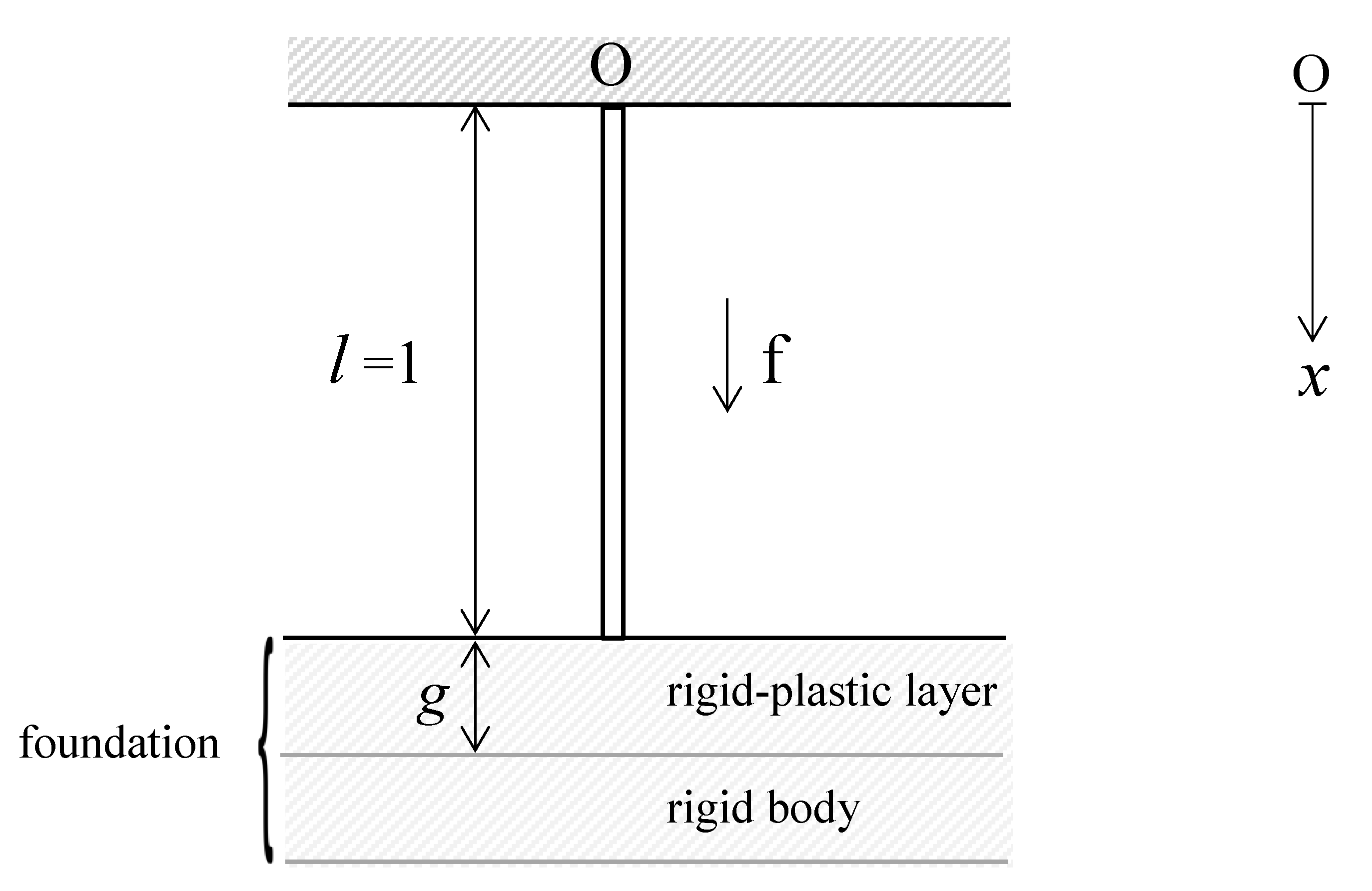
This section illustrates our theoretical results and studies a representative one-dimensional example, that of a static elastic beam in contact with a two-layered foundation. We chose it since it is easier to explain the main ideas of this work but without the complications that arise in two or three dimensions. Thus, we consider a version of Problem ${\mathcal{P}}_{gF}$, where the elastic beam of length $l=1\left[m\right]$ is rigidly attached at $x=0$ and may come in contact, under the action of a force density (per unit length) $f[kg/s^2]$, with a foundation at $x=1$. The foundation has a deformable layer of the rigid-plastic type of thickness $g\left[m\right]$, which is attached to a rigid body underneath. In the notation above, we have $\Omega =(0,1)$, ${\Gamma }_D=\{x=0\}$, ${\Gamma }_N=\varnothing$, ${\Gamma }_C=\{x=1\}$. The setting is depicted in Figure 3.

We denote by $u=u\left(x\right)$ [m] the displacement, and then the linearized strain field is given by $\epsilon \left(u\right)=u^{\prime }$ (dimensionless), where, here and below, the prime denotes the derivative with respect to $x\in [0,1]$. We denote by Y [kg/m s${}^2$] the Young modulus of the rod’s material, A [m${}^2$] the cross sectional area of the rod, and then $E=YA$ [kg m/s${}^2$] is the effective (1D) Young modulus. The stress in the rod is given by $\sigma \left(x\right)$ [kg m/s${}^2$], and within linearized elasticity, $\sigma =E{u}^{\prime }$. For the sake of simplicity, we assume that $f\in \mathbb{R}$ does not depend on the spatial variable.

The statement of the problem of static contact between an elastic rod and a rigid-plastic foundation is the following.

Problem 12.

${\mathcal{P}}_{gF}^{1d}$. Find a displacement field $u:[0,1]\to \mathbb{R}$ and a stress field $\sigma :[0,1]\to \mathbb{R}$, such that

$$\begin{array}{ccc}& & \sigma \left(x\right)=E{u}^{\prime }\left(x\right)\mathrm{for}x\in (0,1),\hfill \end{array}$$

(90)

$$\begin{array}{ccc}& & {\sigma }^{\prime }\left(x\right)+f=0\mathrm{for}x\in (0,1),\hfill \end{array}$$

(91)

$$\begin{array}{ccc}& & u\left(0\right)=0,\hfill \end{array}$$

(92)

$$\begin{array}{ccc}& & u\left(1\right)\le g,\left.\begin{array}{c}\sigma \left(1\right)=0\mathrm{if}u\left(1\right)<0\hfill \\ -F\le \sigma \left(1\right)\le 0\mathrm{if}u\left(1\right)=0\hfill \\ \sigma \left(1\right)=-F\mathrm{if}0<u\left(1\right)<g\hfill \\ \sigma \left(1\right)\le -F\mathrm{if}u\left(1\right)=g\hfill \end{array}\right\}.\hfill \end{array}$$

(93)

Here, $F[kgm/se{c}^2]$ is the rigid-plastic material yield limit, assumed to be positive. One can combine Equations (1) and (2) into $E{u}^{\prime \prime }+f=0$; however, we write it in this way to conform to the formulation of the abstract problems above.

We proceed to the the variational formulation and analysis of Problem ${\mathcal{P}}_{gF}^{1d}$. To that end, we use the space

$$V=\{v\in H^1(0,1):v\left(0\right)=0\},$$

and the set of admissible displacement fields is defined by

$$K_g=\{u\in V:u\left(1\right)\le g\}.$$

Then, the variational form of Problem ${\mathcal{P}}^{1d}$, obtained using integration by parts, is as follows.

Problem 13.

${\mathcal{P}}_{gF}^{1d-V}$. Find a displacement field $u\in K_g$ such that

$${\int }_0^{1}E{u}^{\prime }(v^{\prime }-u^{\prime })dx+Fv{\left(1\right)}^{+}-Fu{\left(1\right)}^{+}\ge {\int }_0^{1}f(v-u)dx\forall v\in K_g.$$

(94)

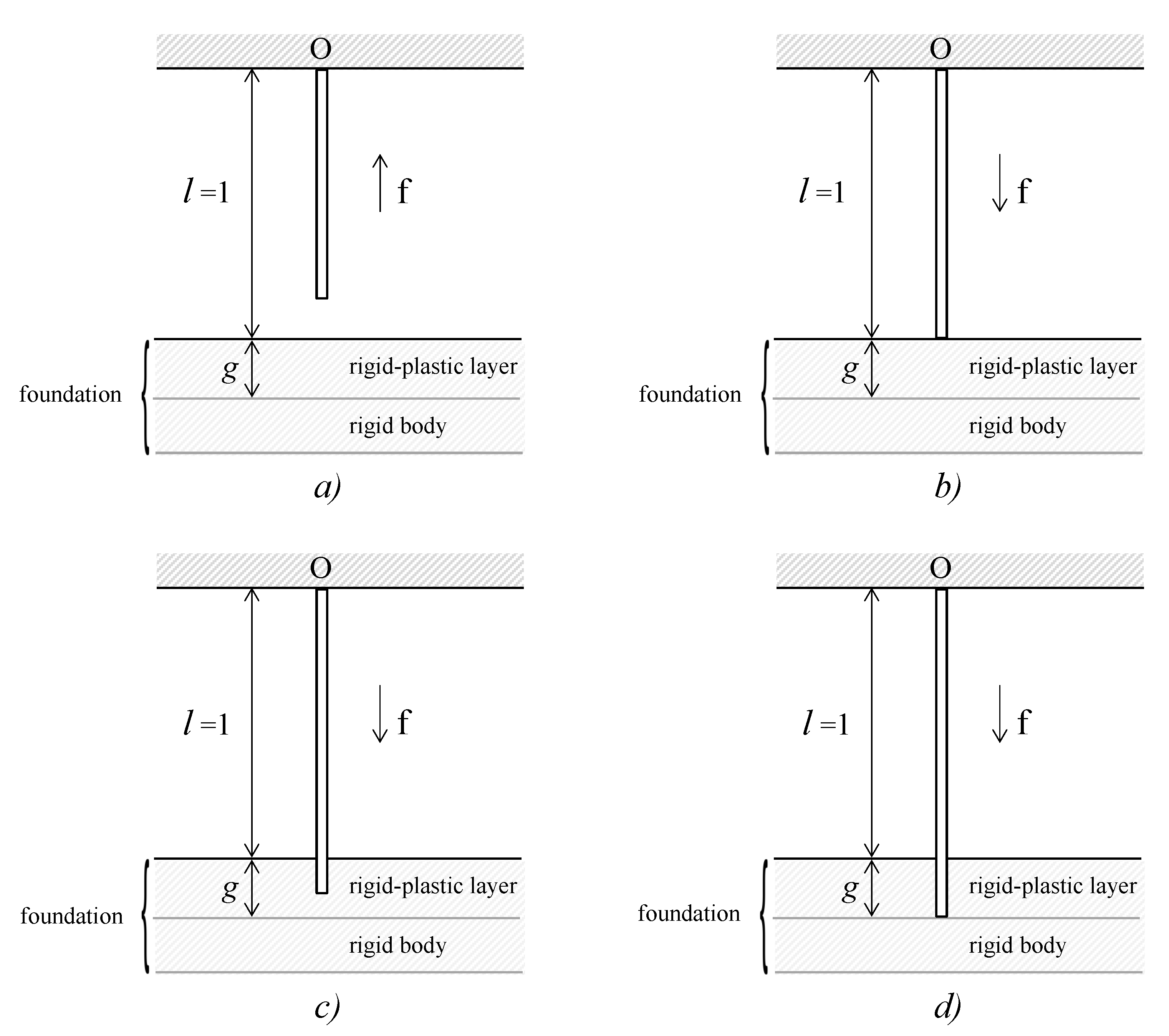
The existence of a unique solution to Problem ${\mathcal{P}}_{gF}^{1d-V}$ follows from Corollary 1(a). However, since the example is “simple”, direct calculations allow us to solve Problem ${\mathcal{P}}_{gF}^{1d}$ and obtain closed form solutions. As was noted above, these may be used to calibrate and verify numerical algorithms for realistic engineering problems. It is found that there are four different possible cases that depend on the relationship between f and F. We describe each one and its corresponding mechanical interpretation.

(a) The case $f<0$. The body force acts away from the foundation and then the solution of Problem ${\mathcal{P}}^{1d}$ is given by

$$\left\{\begin{array}{c}\sigma \left(x\right)=f(1-x),\hfill \\ u\left(x\right)=\frac{f}{E}\left(1-\frac{1}{2}x\right)x,\hfill \end{array}\right.\forall x\in [0,1].$$

(95)

In this case, as is to be expected since there is no contact, $u\left(1\right)<0$ and $\sigma \left(1\right)=0$. Since there is separation between the rod’s end and the foundation, there is no reaction at $x=1$. This case corresponds to Figure 4a.

(b) The case $0\le f<2F$. The force pushes the rod towards the foundation and the solution of Problem ${\mathcal{P}}^{1d}$ is given by

$$\left\{\begin{array}{c}\sigma \left(x\right)=\frac{f}{2}(1-2x),\hfill \\ u\left(x\right)=\frac{f}{2E}\left(1-x\right)x,\hfill \end{array}\right.\forall x\in [0,1].$$

(96)

We have $u\left(1\right)=0$ and $-F<\sigma \left(1\right)\le 0$, which shows that the rod is in contact with the foundation, just touching it, and the reaction of the foundation is towards the rod. Nevertheless, there is no penetration, since the magnitude of the stress at $x=1$ is under the yield limit F and, therefore, the rigid-plastic layer behaves like a rigid layer. This case is depicted in Figure 4b.

(c) The case $2F\le f<2Eg+2F$. In this case, the force is sufficiently large to cause the penetration of the rod’s end into the rigid-plastic layer. The solution of Problem ${\mathcal{P}}^{1d}$ is given by

$$\left\{\begin{array}{c}\sigma \left(x\right)=f(1-x)-F,\hfill \\ u\left(x\right)=\frac{f}{2E}\left(2-x\right)x-\frac{F}{E}x,\hfill \end{array}\right.\forall x\in [0,1].$$

(97)

We have $0\le u\left(1\right)<g$ and $-\sigma \left(1\right)=F$. This, indeed, shows that the stress at $x=1$ reached the yield limit and, therefore, there is penetration into the rigid-plastic layer which now behaves plastically. Nevertheless, the penetration is partial and $u\left(1\right)<g$. This case is shown in Figure 4c.

(d) The case $2Eg+2F\le f$. Here, the applied force is sufficient to make the whole layer plastic. The solution of Problem ${\mathcal{P}}^{1d}$ is given by

$$\left\{\begin{array}{c}\sigma \left(x\right)=\frac{f}{2}(1-2x)+Eg,\hfill \\ u\left(x\right)=\frac{f}{2E}\left(1-x\right)x+g,\hfill \end{array}\right.\forall x\in [0,1].$$

(98)

We have $u\left(1\right)=g$ and $\sigma \left(1\right)\le -F$, which shows that the rigid-plastic layer is completely penetrated and the displacement of the point $x=1$ reaches the rigid body. The magnitude of the reaction in this point is larger than the yield limit F since, besides the reaction of the rigid-plastic layer, there is also the reaction of the rigid body, which becomes active in this case. This case is depicted in Figure 4d).

The analytic forms (95)–(98) of the solution in the four cases show clearly the continuous dependence of the solution on the data F and g, which is the content of Corollary 2(e)–(g). For instance, denote in what follows by $(u_n,{\sigma }_n)$ the solution to Problem ${\mathcal{P}}_{gF}^{1d}$ for $g=g_n>0$ and $F_n=F>0$, for all $n\in \mathbb{N}$. Then, it follows from (95)–(98) that

$$u_n\left(x\right)\to \tilde{u}\left(x\right),{\sigma }_n\left(x\right)\to \tilde{\sigma }\left(x\right)\mathrm{for}\mathrm{all}x\in [0,1]$$

(99)

where $\tilde{u}:[0,1]\to \mathbb{R}$ and $\tilde{\sigma }:[0,1]\to \mathbb{R}$ are the functions defined by

$$\left\{\begin{array}{c}\tilde{\sigma }\left(x\right)=\frac{f}{2}(1-2x),\hfill \\ \tilde{u}\left(x\right)=\frac{f}{2E}\left(1-x\right)x,\hfill \end{array}\right.\forall x\in [0,1]$$

if $f<0$, and

$$\left\{\begin{array}{c}\tilde{\sigma }\left(x\right)=\frac{f}{2}(1-2x),\hfill \\ \tilde{u}\left(x\right)=\frac{f}{2E}\left(1-x\right)x,\hfill \end{array}\right.\forall x\in [0,1]$$

if $f\ge 0$. On the other hand, it is easy to see that the couple $(\tilde{u},\tilde{\sigma })$ is the solution to the Signorini problem without a gap, that is:

Problem 14.

${\mathcal{P}}^{1d}$. Find a displacement field $u:[0,1]\to \mathbb{R}$ and a stress field $\sigma :[0,1]\to \mathbb{R}$, which satisfy (90)–(92) and $u\left(1\right)\le 0$, $\sigma \left(1\right)\le 0$, $\sigma \left(1\right)u\left(1\right)=0$.

Therefore, the convergence (99) represents a validation of the convergence result (84).

8. Conclusions

In this paper, we considered a general mathematical model, actually a framework that describes the equilibrium of a system of a linearly elastic body that is in contact with a number of different types of foundations. The model includes four important particular cases, which depend on the assumptions on the system and its parameters. The variational formulation of the general model is in the form of an elliptic quasivariational inequality for the displacement field of the contacting body. We prove the well-posedness of this inequality with respect to a specific Tykhonov triple, and we use this result to deduce convergence results of the solutions with respect to the parameters. Finally, this unified theory for dealing with the variants of the model with the various contact conditions and these convergence results provides the framework that clearly shows the links and relationships among the weak solutions of the different contact settings and conditions. We also provide a “simple” example with four cases that make the theory transparent and the various concepts about the continuous dependence of the solutions on the data easier to follow. This example has interest in and of itself as it may be used as a benchmark for computer simulations of “real” problems.

Our results in this work can be extended in several directions. First, a more general elastic constitutive law of the form $\mathbf{\sigma }=\mathcal{F}\mathbf{\epsilon }\left(\mathit{u}\right)$, in which $\mathcal{F}$ is a strongly monotone Lipschitz continuous nonlinear operator, can be studied. In such a case, the proof of Theorem 1 can be recovered by using pseudomonotonicity arguments. Second, the dependence of the solution on the density of body forces, density of surface tractions, and coefficient of friction can be obtained, under appropriate assumptions, by using an appropriate choice of ${\epsilon }_n$ in (44). Extensions to quasistatic contact problems with viscoelastic or viscoplastic materials or to contact problems with nonsmooth interface boundary conditions can also be obtained. Steps in this direction have been made in [19,29], where the concept of Tykhonov triple and Tykhonov well-posedness have been used. It also may be of considerable interest to extend the current methodology to include additional processes on the contacting surfaces such as adhesion of damage [7]. Finally, numerical analysis and computer simulations of these theoretical convergence results would be welcome.

Besides the novelty of the results in this paper, we illustrate the use of the new mathematical tools in the variational analysis of contact problems with unilateral constraints. This is an additional reinforcement of one of the main features of the Mathematical Theory of Contact Mechanics, which is the substantial cross fertilization between the models and applications, on one hand, and the nonlinear functional analysis, on the other hand.

References

- Capatina, A. Advances in Mechanics and Mathematics. In Variational Inequalities and Frictional Contact Problems; Springer: New York, NY, USA, 2014; Volume 31. [Google Scholar]
- Duvaut, G.; Lions, J.-L. Inequalities in Mechanics and Physics; Springer: Berlin, Germany, 1976. [Google Scholar]
- Eck, E.; Jarušek, J.; Krbec, M. Pure and Applied Mathematics. In Unilateral Contact Problems: Variational Methods and Existence Theorems; CRC Press: New York, NY, USA, 2005; Volume 270. [Google Scholar]
- Naniewicz, Z.; Panagiotopoulos, P.D. Mathematical Theory of Hemivariational Inequalities and Applications; Marcel Dekker, Inc.: New York, NY, USA, 1995. [Google Scholar]
- Panagiotopoulos, P.D. Inequality Problems in Mechanics and Applications; Birkhäuser: Boston, MA, USA, 1985. [Google Scholar]
- Panagiotopoulos, P.D. Hemivariational Inequalities, Applications in Mechanics and Engineering; Springer: Berlin, Germany, 1993. [Google Scholar]
- Shillor, M.; Sofonea, M.; Telega, J.J. Models and Analysis of Quasistatic Contact; Lecture Notes in Physics; Springer: Berlin, Germany, 2004; Volume 655. [Google Scholar]
- Sofonea, M.; Matei, A. Mathematical Models in Contact Mechanics; London Mathematical Society Lecture Note Series 398; Cambridge University Press: Cambridge, UK, 2012. [Google Scholar]
- Sofonea, M.; Migórski, S. Pure and Applied Mathematics. In Variational-Hemivariational Inequalities with Applications; Chapman & Hall: Boca Raton, MA, USA; CRC Press: London, UK, 2018. [Google Scholar]
- Zavarise, G.; Wriggers, P. (Eds.) Trends in Computational Contact Mechanics; Lecture Notes in Applied and Computational Mechanics; Springer: Berlin, Germany, 2011; Volume 58. [Google Scholar]
- Glowinski, R. Numerical Methods for Nonlinear Variational Problems; Springer: New York, NY, USA, 1984. [Google Scholar]
- Han, W.; Sofonea, M. Studies in Advanced Mathematics. In Quasistatic Contact Problems in Viscoelasticity and Viscoplasticity; American Mathematical Society: Providence, RI, USA; International Press: Somerville, MA, USA, 2002; Volume 30. [Google Scholar]
- Kikuchi, N.; Oden, J.T. Contact Problems in Elasticity: A Study of Variational Inequalities and Finite Element Methods; SIAM: Philadelphia, PA, USA, 1988. [Google Scholar]
- Han, W.; Sofonea, M. Numerical analysis of hemivariational inequalities in Contact Mechanics. Acta Numer. 2019, 28, 175–286. [Google Scholar] [CrossRef] [Green Version]
- Sofonea, M.; Xiao, Y.B. Tykhonov triples, Well-posedness and convergence results. Carphatian J. Math. 2020, in press. [Google Scholar]
- Tykhonov, A.N. On the stability of functional optimization problems. USSR Comput. Math. Math. Phys. 1966, 6, 631–634. [Google Scholar] [CrossRef]
- Sofonea, M.; Tarzia, D.A. On the Tykhonov Well-posedness of an antiplane shear problem. Mediterr. J. Math. 2020, 17, 1–21. [Google Scholar] [CrossRef]
- Sofonea, M. Tykhonov Well-posedness of a rate-type constitutive law. Mech. Res. Commun. 2020, 108, 103566. [Google Scholar] [CrossRef]
- Sofonea, M.; Xiao, Y.B. Tykhonov Well-posedness of a viscoplastic contact problem. J. Evol. Equ. Control Theory 2020, 9, 1167–1185. [Google Scholar] [CrossRef] [Green Version]
- Signorini, A. Sopra alcune questioni di elastostatica. Soc. Ital. Prog. Sci. 1933, 21, 143–148. [Google Scholar]
- Oden, J.T.; Martins, J.A.C. Models and computational methods for dynamic friction phenomena. Comput. Methods Appl. Mech. Eng. 1985, 52, 527–634. [Google Scholar] [CrossRef]
- Klarbring, A.; Mikelič, A.; Shillor, M. Frictional contact problems with normal compliance. Int. J. Eng. Sci. 1988, 26, 811–832. [Google Scholar] [CrossRef]
- Klarbring, A.; Mikelič, A.; Shillor, M. On friction problems with normal compliance. Nonlinear Anal. Theory Methods Appl. 1989, 13, 935–955. [Google Scholar] [CrossRef]
- Martins, J.A.C.; Oden, J.T. Existence and uniqueness results for dynamic contact problems with nonlinear normal and friction interface laws. Nonlinear Anal. Theory Methods Appl. 1987, 11, 407–428. [Google Scholar] [CrossRef]
- Oden, J.T.; Pires, E. Nonlocal and nonlinear friction laws and variational principles for contact problems in elasticity. J. Appl. Mech. 1983, 50, 67–82. [Google Scholar] [CrossRef]
- Duvaut, G. Loi de frottement non locale. J. Méc. Thé. Appl. 1982, 73–78. [Google Scholar]
- Sofonea, M.; Xiao, Y.B. Tykhonov Well-posedness of elliptic Variational-Hemivariational Inequalities. Electron. J. Differ. Equ. 2019, 64, 64. [Google Scholar]
- Sofonea, M.; Matei, A. Advances in Mechanics and Mathematics. In Variational Inequalities with Applications: A Study of Antiplane Frictional Contact Problems; Springer: New York, NY, USA, 2009; Volume 18. [Google Scholar]
- Liu, Z.; Sofonea, M.; Xiao, Y.B. Tykhonov Well-posedness of a frictionless unilateral contact problem. Math. Mech. Solids 2020, 25, 1294–1311. [Google Scholar] [CrossRef]
Figure 1.
Physical setting: (a) contact with a rigid obstacle without gap; (b) contact with a rigid obstacle with gap; (c) contact with a rigid obstacle covered by a deformable layer.
Figure 2.
Five contact conditions with unilateral constraints: (a) condition (1); (b) condition (2); (c) condition (7); (d) condition (9); (e) condition (11).
Figure 3.
Physical setting.
Figure 4.
The four cases of contact between the rod and the foundation: (a) The case ; (b) the case ; (c) the case ; (d) the case .
Publisher’s Note: MDPI stays neutral with regard to jurisdictional claims in published maps and institutional affiliations. |
© 2020 by the authors. Licensee MDPI, Basel, Switzerland. This article is an open access article distributed under the terms and conditions of the Creative Commons Attribution (CC BY) license (http://creativecommons.org/licenses/by/4.0/).
Share and Cite
MDPI and ACS Style
Sofonea, M.; Shillor, M. Tykhonov Well-Posedness and Convergence Results for Contact Problems with Unilateral Constraints. Technologies 2021, 9, 1. https://0-doi-org.brum.beds.ac.uk/10.3390/technologies9010001
AMA Style
Sofonea M, Shillor M. Tykhonov Well-Posedness and Convergence Results for Contact Problems with Unilateral Constraints. Technologies. 2021; 9(1):1. https://0-doi-org.brum.beds.ac.uk/10.3390/technologies9010001
Chicago/Turabian StyleSofonea, Mircea, and Meir Shillor. 2021. "Tykhonov Well-Posedness and Convergence Results for Contact Problems with Unilateral Constraints" Technologies 9, no. 1: 1. https://0-doi-org.brum.beds.ac.uk/10.3390/technologies9010001
Note that from the first issue of 2016, this journal uses article numbers instead of page numbers. See further details here.