A Model of Damage for Brittle and Ductile Adhesives in Glued Butt Joints


1
Laboratory QUARTZ EA7393, Supméca, 93400 Saint-Ouen-sur-Seine, France
2
Department of Engineering, University of Ferrara, 44122 Ferrara, Italy
3
Aix-Marseille Université, CNRS, Centrale Marseille, LMA, 13453 Marseille, France
*
Author to whom correspondence should be addressed.
Technologies 2021, 9(1), 19; https://0-doi-org.brum.beds.ac.uk/10.3390/technologies9010019
Submission received: 9 February 2021
/
Revised: 28 February 2021
/
Accepted: 3 March 2021
/
Published: 6 March 2021
(This article belongs to the Special Issue Advances in Multiscale and Multifield Solid Material Interfaces)
Abstract
:The paper presents a new analytical model for thin structural adhesives in glued tube-to-tube butt joints. The aim of this work is to provide an interface condition that allows for a suitable replacement of the adhesive layer in numerical simulations. The proposed model is a nonlinear and rate-dependent imperfect interface law that is able to accurately describe brittle and ductile stress–strain behaviors of adhesive layers under combined tensile–torsion loads. A first comparison with experimental data that were available in the literature provided promising results in terms of the reproducibility of the stress–strain behavior for pure tensile and torsional loads (the relative errors were less than ) and in terms of failure strains for combined tensile–torsion loads (the relative errors were less than ). Two main novelties are highlighted: (i) Unlike the classic spring-like interface models, this model accounts for both stress and displacement jumps, so it is suitable for soft and hard adhesive layers; (ii) unlike classic cohesive zone models, which are phenomenological, this model explicitly accounts for material and damage properties of the adhesive layer.
1. Introduction
Within the last decades, adhesive bonding became a very common assembly technique in many industrial sectors, such as aeronautical (e.g., in composite aircraft to bond the stringers to fuselage and wing skins to stiffen the structures against buckling [1]), civil (e.g., in glass-fiber-reinforced polymer pultruded beams [2] or in carbon-fiber-reinforced polymer beams [3]), automotive (e.g., in both closures and structural modules [4]), and biomedical engineering (to fix implants in bone tissue in orthopedic or dentistry surgery [5]), as an alternative to conventional joining techniques, such as welding and riveting [6]. Adhesive bonding provides several advantages, including reduced stress concentrations, higher corrosion resistance, water tightness, and the ability to join materials with dissimilar properties. Moreover, this technique is increasingly chosen by the transport industry (automotive and aeronautics) because it allows the production of lighter structures, thus reducing emissions. Nevertheless, adhesive bonding still presents some disadvantages. One of the main concerns limiting the use of adhesive joints is their long-life durability when exposed to service conditions [4]. Corrosion and aging may cause micro-cracking phenomena that can be measured via non-destructive techniques [7]. Another drawback is represented by the multifactorial and multiscale nature of the damage phenomena occurring in the adhesive joints, which make it more complex to predict their strength.
In some structural polymeric adhesives, the tensile stress–strain behavior is typically characterized by an initial linear-elastic phase, followed by softening and rupture. This nonlinear constitutive behavior suggests that a micro-cracking process could occur: pre-existing microcracks, generated by the adhesive preparation (manufacturing, thermal treatment, etc.) and initially present in the linear-elastic phase, propagate during the softening phase, causing debonding and failure [8].
Generally, tube-to-tube butt joints are used to experimentally characterize the mechanical properties of structural adhesives under combined tensile–torsion loads [9,10,11]. Despite numerous experimental studies on this subject, it is still not possible to univocally define the damage/failure behavior of adhesive layers (see the disadvantages listed above). For this reason, a modeling approach can be very useful, and that is what this work proposes.
In numerical modeling, it is often suitable to avoid a volumetric description of the adhesive layer in order to limit problems that can be involved (e.g., a mesh size that is too small, mesh dependency, too large of a number of degrees of freedom, and too long of a computational time). The classic strategy used for modeling damage in adhesive-bonded joints is based on cohesive zone models (CZMs) [6], which are described by a traction–separation (TS) law across the cohesive surface. Several TS laws of different shapes (i.e., bilateral, trapezoidal, polynomial) have been proposed (see [12,13] and the references therein), and they adequately describe the global response of adhesive-bonded joints [14,15,16,17]. However, a crucial drawback of CZMs is that they adopt a phenomenological approach, and thus, the model parameters describing the damage/failure behavior of adhesives are not based on their physical properties (e.g., material properties, geometry).
To overcome this drawback, for the past few years, the authors have been working on alternative TS laws, issued by an imperfect interface approach combining continuum damage mechanics and asymptotic homogenization. These imperfect interface laws have already established their effectiveness in taking into account the micromechanical properties of the adhesive, such as anisotropy [18], micro-cracking, and roughness [19]. Moreover, they can describe the behavior of hard adhesive layers (as stiff as adherents) in which both stress and displacement jumps occur [20,21,22]. Recently, the authors provided a new hard imperfect interface model accounting for micro-cracking damage [23] via an evolution law that is directly related to the mechanical properties of the adhesive.
As a novelty, this paper aims to apply the hard imperfect interface model cited above to the case of adhesive layers in glued butt joints submitted to combined tensile–torsion loads. In detail, a tube-to-tube butt joint configuration is chosen in order to provide an analytical law that, once implemented in a finite element code, can simulate standard characterization tests for structural adhesives.
The presentation of the analytical interface model and its original validation by comparison with experimental data by Murakami et al. [9] are the subjects of this paper, which is organized as follows: the analytical model is presented in Section 2; its numerical implementation together with the chosen experimental data from [9] are detailed in Section 3; the results are illustrated in Section 4, and finally, conclusions and perspectives of future work are highlighted in the summary.
2. Analytical Method for Damage Prediction
After introducing the equilibrium problem of the tube-to-tube butt joint, a classical solution is first introduced, corresponding to the perfect contact between the adherents and modeling a very rigid adhesive. Next, a generalization of the classical solution is proposed, taking into account the presence of a very thin deformable adhesive. The latter is described by a model of an imperfect interface proposed in [22]. Micro-cracking damage within the adhesive is described by using the Kachanov–Sevostianov (KS) model for micro-cracked materials [24,25]. Damage evolution is accounted for by the evolution law obtained in [23] via an asymptotic method.
2.1. Classical Solution for Perfect Contact between the Adherents
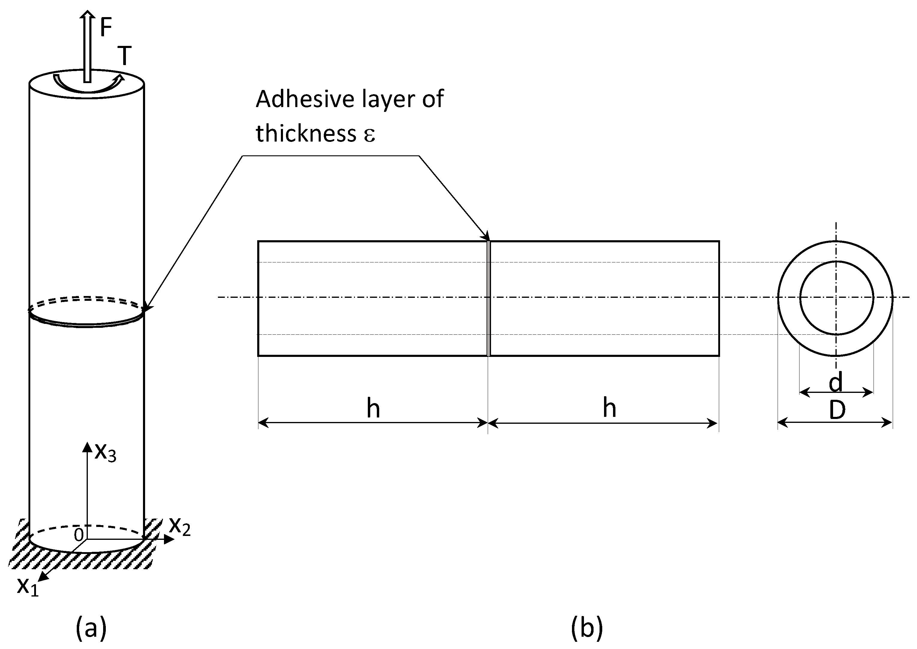
The butt-joint specimen is composed of two identical cylindrical adherents that are joined together. The lower basis of the specimen is fixed, and the upper one is subjected to combined tensile force F and torque as shown in Figure 1, where the dimensions of the adherents are also shown. Under the simplifying hypotheses of perfect adhesion, small strains, and linear-elastic material behavior, the stress tensor in the adherents is given by the classical relation
where is the versor of the i axis, the symbol ⊙ is taken to denote the symmetric dyadic product of vectors, and A and are the cross-sectional area and the polar moment of inertia, respectively. The stress tensor (1) is divergence-free, and the surface forces vanish on the lateral surface of the cylinder, as is the outward normal to the lateral surface. The resultant vertical force and torque on the upper basis of the cylinder balance the applied force F and torque respectively, so equilibrium is ensured.
Assuming the adherents to be made of the same linearly elastic isotropic material with Young’s modulus Poisson’s ratio and shear modulus the homogeneous displacement field in the adherents corresponding to the stress (1) is
2.2. Generalized Equilibrium Solution for Imperfect Contact between the Adherents
The displacement field (2) is appropriate for a specimen made of two identical adherents that are perfectly joined. To take into account the presence of a very thin elastic adhesive without describing it geometrically in a numerical model, we propose the original approach to impose an imperfect interface boundary condition that simulates the macroscopic behavior of a very thin elastic adhesive [20]. Often, structural adhesives have a stiffness that is comparable to the adherents’ stiffnesses; in this case their mechanical behavior cannot be accurately described via a classic spring-like interface model (i.e., the continuity of stresses and discontinuity of displacements), but a hard interface condition also accounting for stress jumps is indicated more. For this reason, we assume the thin adhesive layer to be modeled by the following law of hard imperfect contact proposed in [22]:
where is the thickness of the adhesive, and the symbols and are taken to denote the jump and the average of the quantity across the interface separating the two adherents, respectively; the Greek indexes () are related to the in-plane () quantities; commas denote the first derivatives, and the summation convention is used.
The transmission conditions (3) and (4) prescribe jumps in the traction and displacement fields across the interface between the two adherents, thus describing the asymptotic behavior of a very thin deformable adhesive made of a general anisotropic linear-elastic material with elasticity coefficients which are related to the matrices If the adhesive is modeled as isotropic, with Young’s modulus and Poisson’s ratio the matrices have the form:
To take into account to the presence of the adhesive and enforce the transmission conditions (3) and (4), we propose a generalized equilibrium solution, which is obtained by modifying the displacement field (2) in the upper part of the tube-to-tube butt joint as follows:
where the jumps possibly dependent on have to be determined. In the lower part of the tube-to-tube butt joint below the adhesive, for the displacement field is still given by (2).
In (7), the jumps have to be chosen in order to satisfy the transmission conditions (3) and (4). In the presence of the thin deformable adhesive, assuming that the stress field is still given by (1) and substituting (1) and (5)–(7) into (3) and (4), we obtain:
with
where is the shear modulus of the adhesive.
- The stress field (1), which is continuous across the adhesive and equilibrated by the applied loads;
Notably, the displacement fields above and below the adhesive differ by a rotation in the -plane, given by the jumps and and by a translation along the -axis, given by the jump . The rotation and the translation reproduce the shear and axial deformations, respectively, of a very thin adhesive under the given applied load acting on the tube-to-tube butt joint.
Finally, in the proposed generalized solution that takes the imperfect contact into account, the stress distribution is assumed to be uniform, thus neglecting the effect of stress concentrations on the behavior of the joint. This latter aspect is not addressed in the present paper.
2.3. Micro-Cracking Damaging Adhesive Model
To model a micro-cracking damaging adhesive, we consider the micromechanical homogenization approach proposed by Kachanov and Sevostianov [24,25] based on the approximation of non-interacting micro-cracks. The elastic potential in stresses (complementary energy density) of the effective medium yields the following structure for the effective modulus where M denotes any shear, Young’s, or bulk moduli:
where is the modulus of the undamaged matrix or the initial modulus of the adhesive before damage, is the micro-crack density, thus representing a damage parameter, and the constant C depends on the particular modulus M that is considered and on the orientational distribution of defects. For a two-dimensional random distribution of circular voids, in the Young’s modulus and
in the shear modulus, where is the Poisson ratio of the undamaged matrix [24].
2.4. Damage Evolution
Damage evolution is described as an accumulation of micro-cracks by assuming the damage parameter to increase with time The evolution of the micro-crack density for the proposed model is described by the following kinetic equation, which was proposed in [23]:
where is a positive viscosity parameter, a dot denotes time differentiation, is a strictly negative parameter, is the generalized displacement field defined by (7) above the adhesive and by (2) below it, denotes the positive part, and indicates the component-wise derivative of the stiffness tensor
with respect to . Note that also depends on the adhesive layer thickness .
The kinetic Equation (13) is a first-order ODE in the unknown damage evolution function to be solved for the initial condition . It is important to emphasize that (13) is directly related to the intrinsic mechanical and damage properties of the adhesive layer. In detail, is a damage viscosity that influences the velocity of the damage evolution, and is an energy threshold, which is similar to the energy of adhesion of polymers [26], after which the damage evolution starts at the adhesive layer.
2.5. Stress–Strain Response
The aim here is to find the stress–strain response of the adhesive in the tube-to-tube butt joint subjected to a combined tensile–torsion loading. The tensile stress and shear stress in the adhesive layer are calculated as:
where R is the outer radius of the joint. The tensile strain and shear strain of the adhesive are given by:
respectively, where is the axial displacement of the adhesive and the square root is the circumferential displacement at the outer diameter of the adhesive. Substituting (8) into (16), the normalized tensile stress–tensile strain and shear stress–shear strain are found as follows:
where are given by (9) and (10), respectively. Note that in (9) and (10), the moduli and depend upon the micro-crack density through the KS model (cf. (11)) as follows:
where is the initial shear modulus of the adhesive. The damage parameter evolves via the kinetic Equation (13). By substituting (2), (5)–(7), (14), and (18) into (13) and simplifying, we obtain the following evolution problem for the damage parameter
with
The constants reported in Appendix A, depend on the elasticity coefficients of the adherents on the initial elasticity coefficients of the adhesive and on the constants and Note that tensile and torsion loads are decoupled in (19). Finally, since we are simulating force-controlled tests, the use of (15) allows us to eliminate the tensile load F and the torque T in favor of the control variables and where and are the tensile and shear strain rates, respectively.
For pure torsion, i.e., for and the evolution problem (19) admits the simple solution:
where is the instant at which damage evolution begins:
Substituting (22) and (9) into the second of (17), the shear strain–stress response of the adhesive is obtained:
with
For a pure tensile load, i.e., for and or for a combined tensile–torsion loading, a general closed-form solution of the evolution problem (19) is not available. However, it is possible to obtain a closed-form solution before damage initiation. Indeed, in view of the positivity of the constants and in (20) (cf. the Appendix A), inspection of (19) indicates that the instant of damage initiation for a generic combination of tensile and torsion loads takes the form:
Note that for pure torsion ( and ), (28) reduces to (23).
For the shear stress–strain response is still given by the linear part in (24), while the tensile stress–strain response takes the following linear form:
where the constants are given in Appendix A.
3. Numerical Implementation
The numerical simulations for the pure tensile and for a combined tensile–torsion loading condition were carried out by numerically solving the differential problem (19) using the commercial software Mathematica [27]. For pure torsion loading, the closed-form solution (24) was used. Table 1 and Table 2 show the geometrical and material parameters of the joint specimen of the experimental study by Murakami and coworkers [9] that were chosen to compare with those of the proposed model as an original validation. In [9], the adherents were two S45C carbon steel cylinders joined by a one-component epoxy adhesive (XA7416, 3M Japan Ltd., Tokyo, Japan).
The micromechanical parameters and in (18) were chosen to be equal to and to respectively, the latter value being estimated using (12). The other micromechanical parameters, i.e., the initial value of the damage parameter the viscosity parameter and the energy threshold will be identified in the next subsections starting from the experimental data from [9].
According to [9], two different stress rates were considered in the numerical analyses: MPa/s for the quasi-static (QS) condition and MPa/s for the high-rate (HR) condition.
For pure tensile and torsion tests, the simulations were stopped at failure, i.e., when the stress reached the tensile and shear limit strengths, respectively. For a combined tensile–torsion test, the tensile and shear stresses were related using a loading angle :
4. Results and Discussion
In what follows, a first validation of the proposed model is illustrated. Experimental data obtained in [9] were chosen for comparison in order to highlight the capacity of our model to reproduce the stress–strain behavior of adhesive layers under both pure and combined loads for quasi-static and high-rate loading conditions.
4.1. Simulation of Pure Tensile Tests
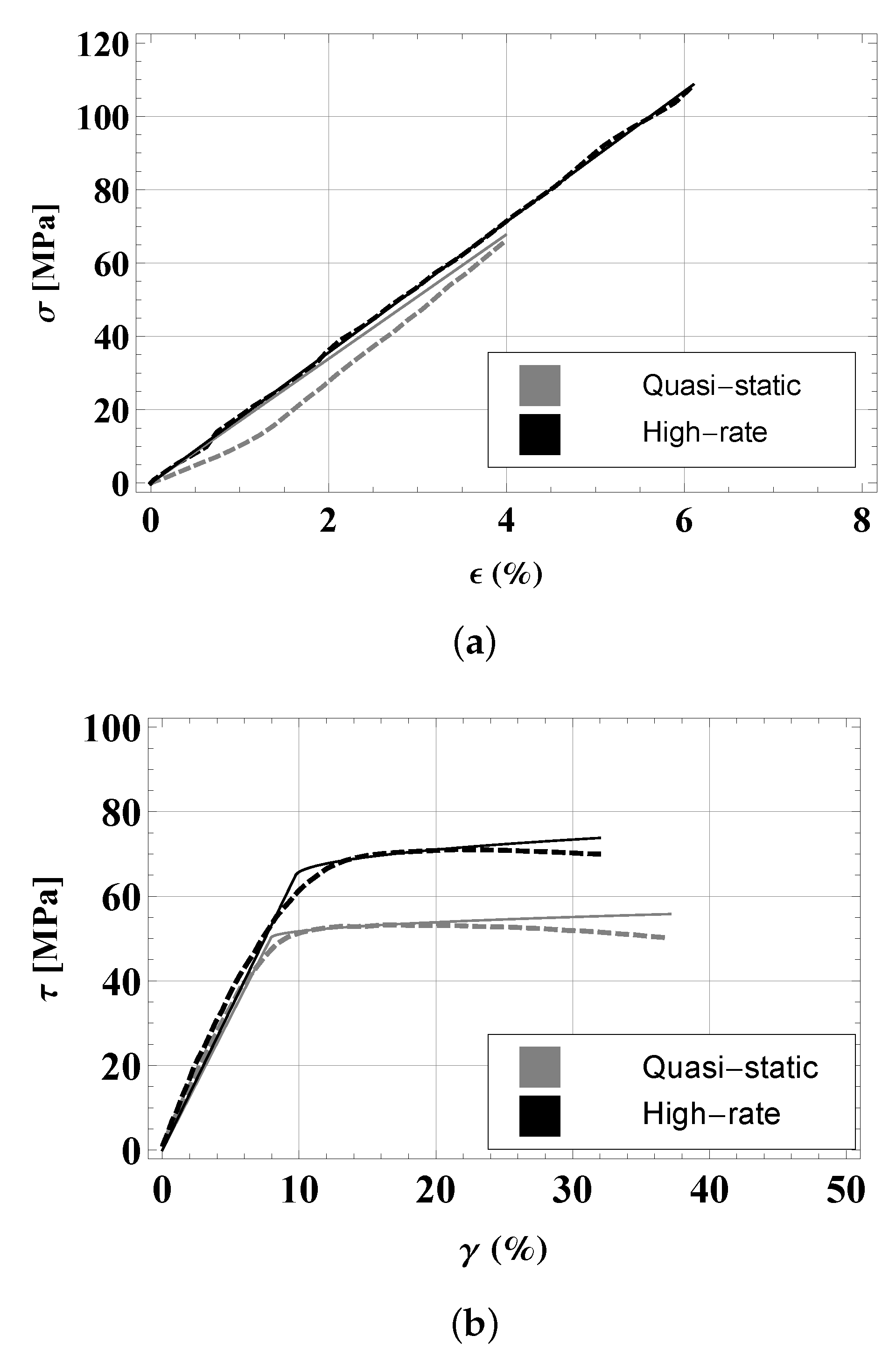
Figure 2a shows the stress–strain curves of the adhesive layer in a pure tensile load obtained by the proposed model for quasi-static (gray) and high-rate (black) loading (solid lines), compared with the experimental curves by [9] (dashed lines). The experimental data were extracted from Figure 9 in [9] by using the free online software WebPlotDigitizer [28].
In view of the modeling approach proposed in the present paper, the experimental curves in Figure 2a can be interpreted as a linear stress–strain response in analogy with a brittle damage behavior, for which the accumulated damage slightly differs from the initial damage . Accordingly, by fitting the experimental curves in Figure 2a into Mathematica by using a linear model, we obtained the following slopes: MPa for the quasi-static case and MPa for the high-rate case. From (29), the initial value of the damage parameter, was calculated as follows:
- for the QS case;
- for the HR case.
These two values are very close. Accordingly to our model, this would indicate a very similar micro-crack density in the samples tested in [9], both in quasi-static and high-rate loading conditions.
Thus, the proposed model is fully able to reproduce the stress–strain behavior under pure tensile loading. Moreover, it is able to catch the influence of the loading rate that was found experimentally in [9], meaning that the tensile strength is higher for high-rate load. It is important to emphasize that this brittle damage behavior of structural adhesive layers under tensile loads has been found in other experimental work, such as that of [11,29].
4.2. Simulation of Pure Torsion Tests
Figure 2b shows the stress–strain curves of the adhesive layer under a pure torsional load obtained with the proposed model for quasi-static (gray) and high-rate (black) loading (solid lines) compared with the experimental curves by [9] (dashed lines). The experimental data were extracted from Figure 10 in [9] by using the free online software WebPlotDigitizer [28].
By fitting the experimental data into Mathematica by using a nonlinear model based on (24), the following values were obtained for the parameters , and
- MPa MPa MPa for the QS case;
- MPa MPa MPa for the HR case.
Substituting these data into (25)–(27), the following values of the parameters , , and were calculated:
- Ns/m, N/m for the QS case;
- Ns/m, N/m for the HR case.
The theoretical curves were stopped at the failure strains— for the QS case and for the HR case. As a result, the relative errors between the experimental values (reported in Table 3 for pure torsion, i.e., for ) and theoretical failure strengths are equal to in the QS case and in the HR case. On the other hand, after damage initiation, i.e., for , both experimental curves exhibited a softening behavior, which cannot be reproduced by the force-controlled theoretical model.
Both the experimental and theoretical stress–strain curves under pure torsion are typical of a ductile damage behavior of the structural adhesive. The proposed model is thus clearly able to accurately reproduce this kind of behavior in terms of both yielding and failure stresses. A ductile damage behavior of structural adhesives in tube-to-tube butt joints is commonly found in torsion experiments (see, for example, the work by Kosmann and coworkers [10]). In addition, in the case of pure torsional tests, the yielding and the failure stresses for the high-rate load were higher than those for the quasi-static load (of almost according to [9]), and the proposed model was able to catch this experimental finding.
4.3. Simulation of Combined Tensile–Torsion Tests
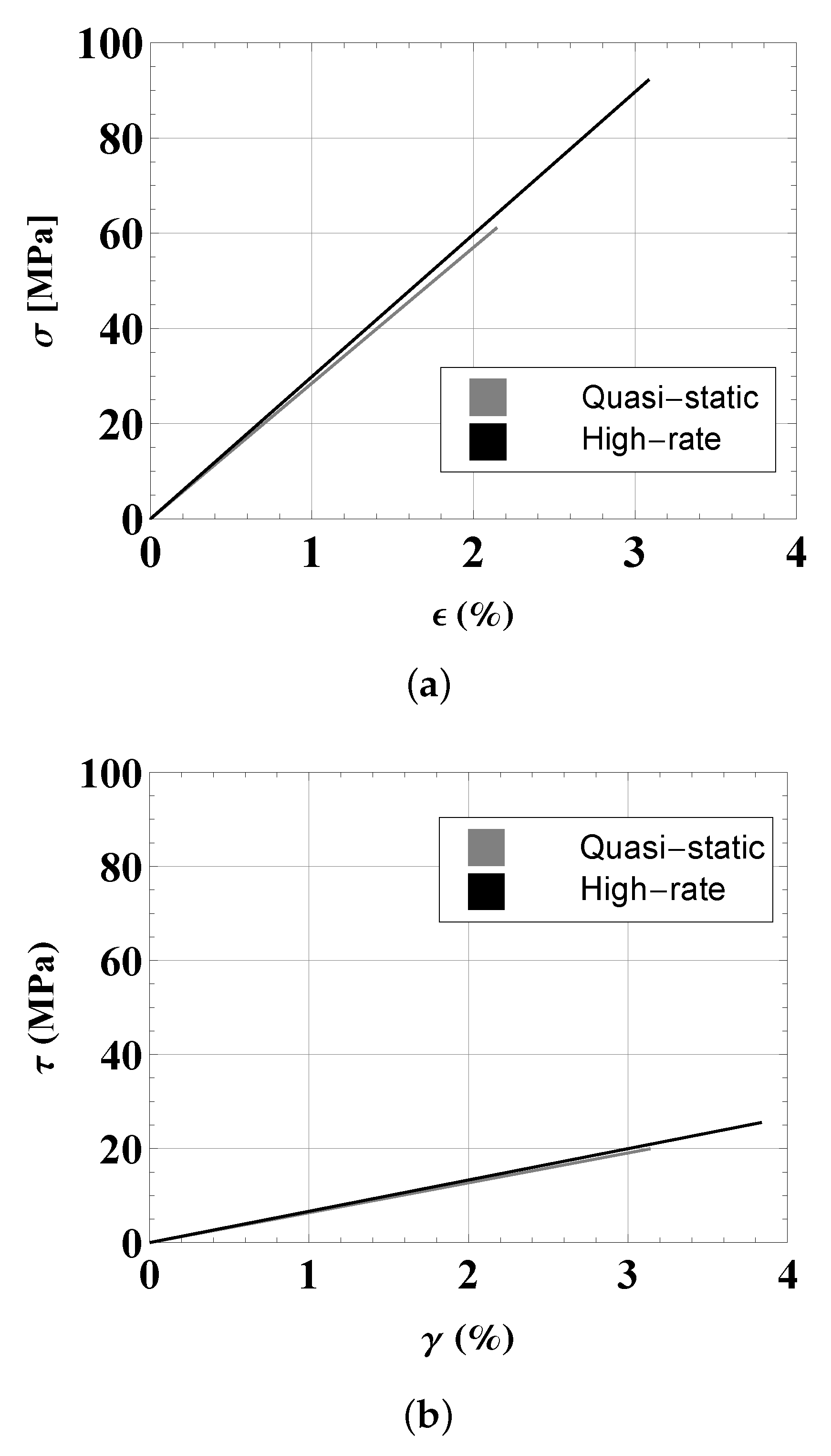
Using the values of the micromechanical parameters , and identified in the previous subsections for the pure loading cases, it was possible to solve the damage evolution problem (19) and plot the corresponding stress–strain diagrams for a combined tensile–torsion load. In particular, the experimental combined loading conditions from [9] for under a QS load and for under an HR load (see Table 3) were selected to be simulated via the proposed analytical model. The limit strengths in the tensile and shear conditions were set up to stop simulations in the stress-controlled mode, and the failure strains in tension and shear were obtained. The simulated stress–strain curves are plotted in Figure 3; the tensile part is shown in Figure 3a and the torsional part in Figure 3b. The corresponding experimental stress–strain curves are not available in [9], so a direct comparison was not possible. However, it was possible to compare the values of the strains at failure. For the QS loading condition (), the simulations gave failure strains of in tension and in torsion, providing acceptable relative errors ( and ) when compared to the failure strains estimated experimentally ( and ). For the HR loading condition (), the simulations gave failure strains of in tension and in torsion, again providing acceptable relative errors ( and ) when compared to the failure strains estimated experimentally ( and ).
Finally, the simulated stress–strain curves for the combined tensile–torsion load exhibited a brittle damage behavior. Unfortunately, it was not possible to find experimental curves in the literature in order to make a comparison, so this and related aspects will be investigated in further work.
5. Summary
The behavior of thin adhesive layers in butt joints under combined tensile and torsion loads was modeled by using an imperfect interface approach that merged continuum damage mechanics and asymptotic homogenization. The proposed approach took micro-cracking damage evolution into account, resulting in a ductile stress–strain behavior of the adhesive for the pure torsional tests and in a brittle stress–strain behavior for the pure tensile and combined tensile–torsion tests. In the case of pure torsion (ductile damage behavior), a closed-form solutions was proposed. In the case of brittle damage behavior (pure tensile and combined tensile–torsion loads), a closed-form solution was calculated in the linear stress–strain domain. The comparisons with the experimental data from [9] gave satisfying results in terms of the failure strains for pure and combined loads in both QS and HR conditions. In all cases, the relative errors between the experimental and simulated failure strains were found to be less than .
The proposed model has some main limitations. First, stresses in the adhesive layer are supposed to be uniformly distributed. This is not realistic, particularly at the boundaries between the adhesive and adherents, where stress concentrations are known to occur [11]; therefore, the effect of the stress concentration on tensile strength is not discussed in this paper. Next, for the sake of simplicity, the adhesive thickness was assumed to be constant and uniform in the whole layer, and perfect thickness uniformity is almost impossible to achieve in real applications. Nevertheless, it is possible to easily generalize the analytical model by accounting for a smooth–rough interface (cf. [19]). Lastly, the viscoplasticity and viscoelasticity that are typical of structural adhesives were not considered in the proposed model. These aspects could be the object of further work.
Despite these limitations, the model is able to accurately reproduce experimental stress–strain behavior for both brittle and ductile damages. Future studies will focus on an experimental protocol for the identification of the model parameters.
Author Contributions
Conceptualization, all authors; methodology, M.L.R. and R.R.; software, M.L.R. and R.R.; validation, all authors; formal analysis, R.R.; investigation, all authors; resources, R.R.; data curation, M.L.R.; writing—original draft preparation, M.L.R. and R.R.; writing—review and editing, M.L.R. and R.R.; visualization, M.L.R. and R.R.; supervision, F.L. and R.R.; project administration, F.L.; funding acquisition, F.L. All authors have read and agreed to the published version of the manuscript.
Funding
This research was funded by the University of Ferrara through FAR grants (2020 and 2021, R.R.).
Institutional Review Board Statement
Not applicable.
Informed Consent Statement
Not applicable.
Data Availability Statement
No new data were created or analyzed in this study. Data sharing is not applicable to this article.
Conflicts of Interest
The authors declare no conflict of interest.
Appendix A
In the case of a bi-dimensional circular defect, one has and , and the constants and simplify to:
Assuming the constants and are positive, and is negative.
For and , the constants and specialize as
References
- Higgins, A. Adhesive bonding of aircraft structures. Int. J. Adhes. Adhes. 2000, 20, 367–376. [Google Scholar] [CrossRef]
- Maurel-Pantel, A.; Lamberti, M.; Raffa, M.L.; Suarez, C.; Ascione, F.; Lebon, F. Modelling of a GFRP adhesive connection by an imperfect soft interface model with initial damage. Compos. Struct. 2020, 239, 112034. [Google Scholar] [CrossRef]
- Kawecki, B.; Podgórski, J. The Effect of Glue Cohesive Stiffness on the Elastic Performance of Bent Wood–CFRP Beams. Materials 2020, 13, 5075. [Google Scholar] [CrossRef]
- Cavezza, F.; Boehm, M.; Terryn, H.; Hauffman, T. A Review on Adhesively Bonded Aluminium Joints in the Automotive Industry. Metals 2020, 10, 730. [Google Scholar] [CrossRef]
- Sokolowski, G.; Krasowski, M.; Szczesio-Wlodarczyk, A.; Konieczny, B.; Sokolowski, J.; Bociong, K. The Influence of Cement Layer Thickness on the Stress State of Metal Inlay Restorations—Photoelastic Analysis. Materials 2021, 14, 599. [Google Scholar] [CrossRef]
- Ramalho, L.D.C.; Campilho, R.D.S.G.; Belinha, J.; Da Silva, L.F.M. Static strength prediction of adhesive joints: A review. Int. J. Adhes. Adhes. 2020, 96, 102451. [Google Scholar] [CrossRef]
- Rucka, M.; Wojtczak, E.; Lachowicz, J. Damage imaging in Lamb wave-based inspection of adhesive joints. Appl. Sci. 2018, 8, 522. [Google Scholar] [CrossRef] [Green Version]
- Chai, H. Observation of deformation and damage at the tip of cracks in adhesive bonds loaded in shear and assessment of a criterion for fracture. Int. J. Fract. 1993, 60, 311–326. [Google Scholar]
- Murakami, S.; Sekiguchi, Y.; Sato, C.; Yokoi, E.; Furusawa, T. Strength of cylindrical butt joints bonded with epoxy adhesives under combined static or high-rate loading. Int. J. Adhes. Adhes. 2016, 67, 86–93. [Google Scholar] [CrossRef]
- Kosmann, J.; Klapp, O.; Holzhüter, D.; Schollerer, M.J.; Fiedler, A.; Nagel, C.; Hühne, C. Measurement of epoxy film adhesive properties in torsion and tension using tubular butt joints. Int. J. Adhes. Adhes. 2018, 83, 50–58. [Google Scholar] [CrossRef]
- Spaggiari, A.; Castagnetti, D.; Dragoni, E. Mixed-mode strength of thin adhesive films: Experimental characterization through a tubular specimen with reduced edge effect. J. Adhes. 2013, 89, 660–675. [Google Scholar] [CrossRef]
- Zhang, J.; Wang, J.; Yuan, Z.; Jia, H. Effect of the cohesive law shape on the modelling of adhesive joints bonded with brittle and ductile adhesives. Int. J. Adhes. Adhes. 2018, 85, 37–43. [Google Scholar] [CrossRef]
- Campilho, R.D.; Banea, M.D.; Neto, J.A.B.P.; da Silva, L.F. Modelling adhesive joints with cohesive zone models: Effect of the cohesive law shape of the adhesive layer. Int. J. Adhes. Adhes. 2013, 44, 48–56. [Google Scholar] [CrossRef] [Green Version]
- Hu, C.; Huang, G.; Li, C. Experimental and Numerical Study of Low-Velocity Impact and Tensile after Impact for CFRP Laminates Single-Lap Joints Adhesively Bonded Structure. Materials 2021, 14, 1016. [Google Scholar] [CrossRef] [PubMed]
- Yu, G.; Chen, X.; Zhang, B.; Pan, K.; Yang, L. Tensile-Shear Mechanical Behaviors of Friction Stir Spot Weld and Adhesive Hybrid Joint: Experimental and Numerical Study. Metals 2020, 10, 1028. [Google Scholar] [CrossRef]
- Liljedahl, C.D.M.; Crocombe, A.D.; Wahab, M.A.; Ashcroft, I.A. Modelling the environmental degradation of adhesively bonded aluminium and composite joints using a CZM approach. Int. J. Adhes. Adhes. 2007, 27, 505–518. [Google Scholar] [CrossRef]
- Pirondi, A.; Moroni, F. Improvement of a Cohesive Zone Model for Fatigue Delamination Rate Simulation. Materials 2019, 12, 181. [Google Scholar] [CrossRef] [Green Version]
- Lebon, F.; Dumont, S.; Rizzoni, R.; López-Realpozo, J.C.; Guinovart-Díaz, R.; Rodríguez-Ramos, R.; Bravo-Castillero, J.; Sabina, F.J. Soft and hard anisotropic interface in composite materials. Compos. Part Eng. 2016, 90, 58–68. [Google Scholar] [CrossRef] [Green Version]
- Dumont, S.; Lebon, F.; Raffa, M.L.; Rizzoni, R. Towards nonlinear imperfect interface models including microcracks and smooth roughness. Ann. Solid Struct. Mech. 2017, 9, 13–27. [Google Scholar] [CrossRef] [Green Version]
- Benveniste, Y.; Miloh, T. Imperfect soft and stiff interfaces in two-dimensional elasticity. Mech. Mater. 2001, 33, 309–323. [Google Scholar] [CrossRef]
- Furtsev, A.; Rudoy, E. Variational approach to modeling soft and stiff interfaces in the Kirchhoff-Love theory of plates. Int. J. Solids Struct. 2020, 202, 562–574. [Google Scholar] [CrossRef]
- Rizzoni, R.; Dumont, S.; Lebon, F.; Sacco, S. Higher order model for soft and hard interfaces. Int. J. Solids Struct. 2014, 51, 4137–4148. [Google Scholar] [CrossRef]
- Raffa, M.L.; Lebon, F.; Rizzoni, R. A micromechanical model of a hard interface with micro-cracking damage. 2021; In Preparation. [Google Scholar]
- Kachanov, M. Elastic solids with many cracks and related problems. Adv. Appl. Mech. 1994, 30, 259–445. [Google Scholar]
- Kachanov, M.; Sevostianov, I. Micromechanics of Materials, with Applications; Springer: Cham, Switzerland, 2018; Volume 249. [Google Scholar]
- Weng, C.; Yang, J.; Yang, D.; Jiang, B. Molecular Dynamics Study on the Deformation Behaviors of Nanostructures in the Demolding Process of Micro-Injection Molding. Polymers 2019, 11, 470. [Google Scholar] [CrossRef] [Green Version]
- Wolfram Research, Inc. Mathematica; Version 12.2; Wolfram Research, Inc.: Champaign, IL, USA, 2020. [Google Scholar]
- Ankit Rohatgi. WebPlotDigitizer. Version: 4.4. November 2020. Available online: https://automeris.io/WebPlotDigitizer (accessed on 28 December 2020).
- Costa-Mattos, H.S.; Monteiro, A.H.; Sampaio, E.M. Modelling the strength of bonded butt-joints. Compos. Part B Eng. 2010, 41, 654–662. [Google Scholar] [CrossRef]
Figure 1.
(a) Sketch of the tube-to-tube joint with the loading configuration. (b) Longitudinal and traversal sections with dimensions.
Figure 1.
(a) Sketch of the tube-to-tube joint with the loading configuration. (b) Longitudinal and traversal sections with dimensions.

Figure 2.
Stress–strain curves in pure loading conditions: (a) Stress–strain curves of the adhesive layer under a pure tensile load obtained with the proposed model for quasi-static and high-rate loading (solid lines) compared with experimental curves by [9] (dashed lines). (b) Stress–strain curves of the adhesive layer under a pure torsion load obtained with the proposed model for quasi-static and high-rate loading (solid lines) compared with experimental curves by [9] (dashed lines).

Figure 3.
Stress–strain curves in combined tensile–torsion loading conditions: (a) Tensile stress–strain curves of the adhesive layer obtained with the proposed model for quasi-static and high-rate loading. (b) Torsion stress–strain curves of the adhesive layer obtained with the proposed model for quasi-static and high-rate loading.


Table 1.
Geometrical parameters of the joint specimen [9].
Table 1.
Geometrical parameters of the joint specimen [9].
| Quantity | Symbol | Value | Unit |
|---|---|---|---|
| Outer diameter | D | 26.0 | mm |
| Inner diameter | d | 20.0 | mm |
| Adhesive thickness | 0.3 | mm |
Table 2.
Mechanical properties of the joint materials [9].
Table 2.
Mechanical properties of the joint materials [9].
| Quantity | Symbol | Value | Unit |
|---|---|---|---|
| Adhesive Young’s modulus | 4.53 | GPa | |
| Adhesive Poisson’s ratio | 0.36 | – | |
| Adherents’ Young’s modulus | E | 200.00 | GPa |
| Adherents’ Poisson’s ratio | 0.30 | – |
Table 3.
Experimentally estimated tensile and torsional (shear) strengths of butt-joint specimens studied in [9].
Table 3.
Experimentally estimated tensile and torsional (shear) strengths of butt-joint specimens studied in [9].
| Loading Rate | Loading Angle [deg.] | Tensile Strength [MPa] | Shear Strength [MPa] | Failure Strain in Tension [%] | Failure Strain in Shear [%] |
|---|---|---|---|---|---|
| QS | 0 | 61.8 | – | 4.0 | – |
| HR | 0 | 90.0 | – | 6.1 | – |
| QS | 90 | – | 53.2 | – | 37.0 |
| HR | 90 | – | 70.0 | – | 32.0 |
| QS | 61.0 | 19.9 | 2.15 | 2.85 | |
| HR | 92.1 | 25.5 | 3.55 | 3.69 |
Publisher’s Note: MDPI stays neutral with regard to jurisdictional claims in published maps and institutional affiliations. |
© 2021 by the authors. Licensee MDPI, Basel, Switzerland. This article is an open access article distributed under the terms and conditions of the Creative Commons Attribution (CC BY) license (http://creativecommons.org/licenses/by/4.0/).
Share and Cite
MDPI and ACS Style
Raffa, M.L.; Rizzoni, R.; Lebon, F. A Model of Damage for Brittle and Ductile Adhesives in Glued Butt Joints. Technologies 2021, 9, 19. https://0-doi-org.brum.beds.ac.uk/10.3390/technologies9010019
AMA Style
Raffa ML, Rizzoni R, Lebon F. A Model of Damage for Brittle and Ductile Adhesives in Glued Butt Joints. Technologies. 2021; 9(1):19. https://0-doi-org.brum.beds.ac.uk/10.3390/technologies9010019
Chicago/Turabian StyleRaffa, Maria Letizia, Raffaella Rizzoni, and Frédéric Lebon. 2021. "A Model of Damage for Brittle and Ductile Adhesives in Glued Butt Joints" Technologies 9, no. 1: 19. https://0-doi-org.brum.beds.ac.uk/10.3390/technologies9010019
Note that from the first issue of 2016, this journal uses article numbers instead of page numbers. See further details here.