Impacts of Overall Financial Development, Access and Depth on Income Inequality

Abstract

There is dense literature on the relationship between financial sector development (FSD) and income inequality. However, most of these studies employ a depth measure of FSD. This study argues that different components of FSD have a heterogenous impact on income inequality. This study first empirically tests the overall impact of FSD on income inequality. Thereafter, I investigate both the linear and nonlinear impact of financial sector development dimensions (depth and access) on income inequality. The study’s novelty lies in using financial access data such as ATM per adult and financial access index and comparing their impact on income inequality versus the impact of financial sector depth (growth in domestic credit) on inequality. Adding to this, fewer studies have investigated the overall impact of FSD. To solve the endogenous problem, the study uses the system General Method of Moments (GMM) on the panel data of 120 countries, from 2004 to 2019. The findings of the study are threefold. Firstly, the study finds that the overall FSD index, individual financial institutions, and market development index all narrow income inequality. Secondly, this study finds that different dimensions of FSD have heterogenous impacts on income inequality, where increased access to financial services reduces income inequality in both linear and nonlinear models. While financial sector depth narrows income inequality in the linear model, the nonlinear model reveals that the Too Much Finance hypothesis holds, as the results confirm a U-shaped relation with income inequality. These results are important for policy decisions concerning financial reforms and income distribution. These results imply that financial sector reforms can be shaped to reduce income inequality by increasing access to credit and through credit policy provisions.

1. Introduction

Increasing income inequality has been at the forefront of public debate. For instance, alleviating income inequality is goal number ten of the Sustainable Development Goals (SDGs) for the 2030 Agenda of the United Nations. Subsequently, policymakers worldwide are concerned about rising income inequality’s economic and social consequences. This paper aims to show that financial sector development (FSD) can be one of the tools for reducing income inequality. FSD has been rising, with advanced countries leading and developing countries catching up. Financial institutions have grown, in volumes of trade and geographical presence. As the financial sector grows, so does the complexity and the number of financial instruments. Borderless banks seen in the present era continue to prosper. It is natural to study their effects on income distribution as FSD affects the economic opportunities of individuals. According to theoretical and empirical literature, financial institutions and markets shape the gap between rich and poor (1) by determining who receives a loan to start a business or finance education (access to human capital financing), (2) through capital rent/profit accumulation, (3) by promoting the participation of poor households in economic activity and helping them to reduce economic vulnerabilities, and (4) through the composition of labor demand.

In addition, access to the financial sector represents inequality of opportunity. For example, rural area residents, women and poor households are the most unbanked households. Consequently, strengthening access to financial services, especially for the poor, is one of the main tools for achieving goal 8 (Economic growth and descent work) of the UN SDGs. Increased access to financial services was the focus of the World Bank Groups Universal Financial Access 2020 initiative, as financial inclusion can boost economic growth and reduce income inequality by mobilizing savings and fostering the formalization of labor and firms.

As such, the main goal of this paper is to investigate the overall impact and different components of FSD on income inequality. Thus, this paper attempts to contribute to the following questions: (i) What is the overall impact of FSD on income inequality? (ii) How does financial sector depth (growth in domestic credit) affect income inequality? (iii) How does increased access to financial services affect income inequality? Empirical results from these questions can be informative for financial sector reform and fair shared prosperity. It is pivotal to ask what the gains from FSD are and who is benefiting the most from these developments. This concern is reasonable as there are far greater negative consequences for macro-stabilities in cases where financial system assets are concentrated. Subsequently, this study hypothesizes that, on average, FSD reduces income inequality, while different dimensions of FSD can produce different impacts on income inequality.

Thus, the study contributes to the available literature by distinguishing the contribution of overall FSD, financial depth and access to income inequality. This is because there are very few studies investigating the impact of FSD. Adding to this, according to my knowledge, no study has empirically tested the development impact of financial institutions and market indexes on income inequality. The study is carried out on yearly data from 2004 to 2019, and the system GMM methodology is employed. The applied robust methodology also serves as a contribution to the mixed literature. Robust system GMM is advantageous over difference GMM as it offers lower variance and bias. Robust system GMM also offers efficient and robust heteroscedasticity and autocorrelation results. Subsequently, the study finds that overall FSD reduces income inequality, chiefly through access to financial institutions rather than through financial markets. Again, the study finds that financial institution depth tends to have a significant impact on income inequality, while financial market depth has no significant impact.

The rest of the paper is organized as follows: Section 2 covers the theoretical framework and review of the literature, including the stylized facts of FSD and income inequality. Section 3 discusses the data collection and methodology. Section 4 presents the results. Section 5 and Section 6 provide a discussion on the implications of the findings, and the conclusions, respectively.

2. Theoretical Framework and Review of Literature

2.1. Theoretical Framework

For the theoretical framework, I begin the analysis by building on the outstanding work of Demirguc-Kunt and Levine (2009), specifically focusing on their contribution to finance in theories of persistent inequality. By decomposing total income into income from labor and physical capital (see Equation (1) below), we can analyze how FSD can affect inequality (Demirguc-Kunt and Levine 2009).

Total inequality = Labor income inequalities + physical capita inequality

(1)

Equation (1) was proposed by Demirguc-Kunt and Levine (2009) and Piketty (2014). The argument is as follows: wage income accounts for around 70 per cent of income inequality and is highly correlated with human capital development (Demirguc-Kunt and Levine 2009; Francese and Mulas-Granados 2015). Meanwhile, income from physical capital magnifies inequality through rent seeking (Demirguc-Kunt and Levine 2009; Piketty 2014; Mihalyi and Szelenyi 2019). The argument is that inequalities from physical capital are larger than from labor income. For example, Piketty (2014) focused on the rent earned by the top 1% income group and postulated that inheritance wealth, capitalist environment and profit growth exacerbate inequality. In contrast, Mihalyi and Szelenyi (2019) emphasize the rent accruing in the top 20% income group and distinguish different types of rent in the capital system. Different from the work of Piketty (2014), Mihalyi and Szelenyi (2019) place a distinction between profits and rent. From this distinction, Mihalyi and Szelenyi (2019) find that higher profits and wage income positively affect economic growth, while rent growth lowers it. Subsequently, the theories of persistent inequality in financial sector development are discussed concerning wage and physical capital income inequalities. Demirguc-Kunt and Levine (2009) argue that financial institutions’ imperfection (e.g., information and contract costs that hinder investment screening and monitoring of financial contracts) outlines the dynamics of inequality, such as wealth and education accumulation.

The difference between skilled versus unskilled labor income is the main direct source for rising income inequality, as wage income typically reflects an individual’s education level. In a perfect credit market, parents’ education and wealth are unimportant as a household can borrow to finance education (Demirguc-Kunt and Levine 2009). Meanwhile, in the presence of imperfect credit markets on education investment, inequality of opportunity explains the distribution of skills. Parents’ education and wealth constrain next generations' access to credit for human capital. Thus, borrowing constraints negatively impact human capital accumulation in the absence of public education. This creates a gap in human capital accumulation, increasing wage inequality (Demirguc-Kunt and Levine 2009). At the same time, increased access to financial services for education investment to poor households who were previously excluded reduces income inequality through human capital accumulation (Galor and Zeira 1993; Demirguc-Kunt and Levine 2009).

On the other hand, the developed financial sector can curb shocks to poor households’ income by allowing them to continue investing in human capital instead of opting for low-skill employment when hit by income shocks. Thus, the developed financial sector helps households to smooth income shocks (Demirguc-Kunt and Levine 2009). FSD lacking increased access to financial services can increase inequality as the sector only caters to selected individuals with financial investment (Greenwood and Jovanovic 1990). Increasing financial institution size and innovation can boost economic growth, pushing up the labor market demand, signifying that the effects of FSD on labor market demand and income inequality are a double-edged sword, in the sense that FSD increases the demand for only skilled labor and magnifies income inequality (Demirguc-Kunt and Levine 2009; Piketty 2014). FSD also increases wage inequality between sectors. For example, the compensation of portfolio managers increases with the complexity of the financial instrument, and in addition, their bonus compensation is usually based on profits. For instance, in Europe, employees of the financial sector are concentrated in the upper end of the income distribution. Denk (2015) emphasizes how financial sector employees receive rent through wage premia and over-skilling. According to Denk (2015), financial sector employees receive exponential earnings/bonuses (wage premia), more so than employees in other sectors, who make roughly the same profit for their respective firms. In other words, using yearly data of OECD countries, Denk (2015) finds that finance wages are around 50% higher than in other sectors. Thus, in essence, these are not remunerations necessary based on productivity levels but rather rents accruing among financial sector employees—hence, Denk (2015) refers to them as wage premia. As such, wage premia from financial sector employees explain the undesirable relationship between FSD and income inequality. Adding to this, there is still a large gender income gap in the financial sector. For example, in Europe, on average, male employees in the sector earn 22% more than females (Denk 2015). Moreover, in terms of financial inclusion and access, the most unbanked groups are women and uneducated households.

Capital income contains real estate and financial capital; as such, owners of capital benefit greatly from FSD. Generally, physical capital such as bond certificates/share ownership and property embodies more wealth inequality; however, inequality of wealth has a direct transmission to income inequality. For example, wealthy households tend to live in more advanced and developed districts, impacting the quality of schools and other forms of economic opportunities. Education may be centralized or free, but education institutions always allow private funding, which will be coming from the wealthy residents—through such funding, these schools obtain better and more advanced technology than public schools. In the long run, income inequality will also grow due to the gap in skills and human capital development. In addition, middle-income households tend to invest more in property than in financial assets. In contrast, rich households have paid up properties and gained more rent from financial assets such as stock and bonds in the financial markets. This distribution of physical capital suggests that different income groups benefit differently from financial rent.

2.2. Review of Literature

2.2.1. Financial Sector Development and Economic Growth

The link between FSD, economic growth and income inequality is complex as these variables exhibit a bidirectional relationship. For instance, the lending decisions of financial institutions have impacts on education investment, business start-ups and the growth of the small business, which in turn influence real output and inequality. There is large and growing evidence that suggests that FSD plays a substantial role in economic development (Goldsmith 1969; Levine 2004; Gründler and Weitzel 2013; Seven and Coskun 2016; Paun et al. 2019; Ongena and Mendez-Heras 2020). There are positive gains on economic growth when there is growth in the (a) numbers of financial sector branches, (b) stock traded and net foreign assets, (c) financial systems and inclusion (represented by financial access and market sophistication), (d) quality of financial systems such as markets, institutions and financial instruments (Paun et al. 2019; Gural and Lomachynska 2017; Bittencourt 2011; Setiawan 2015; Kapingura 2017; Worku 2014). Other studies also suggest a bidirectional relationship between FSD and growth (Sunde 2012; Oluitan 2012), while some additional studies suggest that the impact of FSD on economic growth depends on the growing private credit ratio on real GDP growth (Ductor and Grechyna 2015). Thus, in developed and developing countries, FSD harms economic growth when there is a speedy growth in private credit without growth in real output. Their findings suggest an optimal level of finance development determined by the economy’s characteristics. Lastly, FSD (improved contracts and market) enlarges economic opportunities, thus accelerating growth and reducing inequality.

2.2.2. Financial Sector Development and Income Inequality

The previous subsections focused on the impact of FSD on economic growth as theories of growth overlap those of inequality. Next, I show that there is no consensus in the empirical literature of FSD and income inequality. The bulk of the literature on FSD and income inequality is large. However, as Demirguc-Kunt and Levine (2009) highlighted, the literature lacks a consensus, and to close the gap, they state that further empirical evidence is needed. The grounds for further research lie in finding precise measures or rules of thumb of the impact of FSD on inequality and growth. This is because the theory mirrors a skeleton of inequality trends due to imperfect credit markets. Additionally, before 2004, there were no global cross-country data on financial access measures. This implies that before the year 2004, there were limited global studies on how financial access affects inequality. Simultaneously, the literature on the impacts of financial depth on economic growth and inequality grew.

The literature on FSD and income inequality is divided into four strands: (1) financial narrowing hypothesis, (2) financial widening hypothesis, (3) inverted U-shaped hypothesis of Greenwood and Jovanovic (1990) and (4) the U-shaped hypothesis. The financial narrowing hypothesis suggests that income inequality declines in the presence of an efficient financial market (Banerjee and Newman 1993; Galor and Zeira 1993). These theories emphasize the exacerbating effects of imperfect credit markets on initial wealth distribution and subsequently long-run impacts on income inequality. The widening financial hypothesis was enriched by the book of (Rajan and Zingales 2003) as the title of Chapter 1 of the book was ‘Does finance benefit only the rich?’ Rajan and Zingales (2003) posit that FSD increases income inequality as its benefits spread to rich households, who had initial access to the credit market. Those who lack collateral view requirements for borrowing as follows: ‘you can borrow provided you do not need’, and connections to credit imply ‘you can borrow provided I know and trust you/your business’ (Rajan and Zingales 2003). They argue for good institutions characterized by better legal enforcement, higher levels of general trust, esteem property rights and the developed market to ensure that finance is for all.

Table 1. The narrowing and widening hypotheses of FSD on income inequality.

	Study	Main Variables in the Model of FSD on Inequality	Geographical Area	Findings
Financial narrowing hypothesis	Beck et al. (2004)	Credit to the private sector by financial intermediaries and poorest quintile income, Gini index. Legal origins, natural resource endowment, religious composition and ethnic fractionalization as instruments for endogeneity.	52 developing and developed countries (1960 to 1999) 1.	Using instrumental variable regression, they found that FSD reduces inequality as it grows faster than average GDP per capita.
	Clarke et al. (2006)	The Gini coefficient and credit to the private sector by financial intermediaries over GDP (private credit). To control Kuznets effects, they include initial real GDP per capita and squared term. Other control variables include: inflation rate, government consumption, ethnolinguistic fractionalization and a measure of the protection of property rights. To control for endogeneity, the legal origins indicator is included.	Using data for 83 developed and developing countries between 1960 and 1995.	The study found that when there is greater/deepened FSD, inequality is less in the long run. The results confirming an inverted U-shaped curve of Greenwood and Jovanovic (1990) were not robust.
	Kapingura (2017)	Gini index. FSD: domestic credit to bank sector as % of GDP, and ATM per 100,000 adults.	South Africa (1990–2012 yearly).	An increase in financial access (ATM) reduces inequality more than increasing financial depth.
	Burgess and Pande (2005) 2	FSD: the number of bank branches per 100 000 persons and number of banks opened in rural versus urban areas.	India (1977–1990).	Using OLS and IV, they found that financial access reduces poverty, especially in rural areas.
	Liang (2008)	Provincial rural Gini index. FSD: constructed rural FSD based on the ratio of total loans to rural GDP.	China, based on provincial data from 1991 to 2000.	The GMM technique showed that increased access to financial services and credit in rural areas reduces inequality.
	Shahbaz and Islam (2011)	Gini index, domestic credit to the private sector by financial intermediaries over GDP and financial stability measures developed by authors.	Pakistan (1971–2005).	Using ADRL methodology, they found that FSD reduces income inequality while financial instability increases inequality.
	Prete (2013)	Growth of Gini. FSD: private credit as the ratio of GDP.	30 countries from 1980 to 2005.	Using panel OLS, they find inequality narrowing.
	Dollar and Kraay (2002)	GDP per capita and mean income in the poorest quintile. Commercial bank assets/total bank assets, human capital. Inflation, trade openness, the rule of law/property rights.	137 countries (1950–1999)	FSD increases inequality by a small magnitude compared to the increasing impact on economic growth.
	Hendel et al. (2005)	Developed a model similar to (Rajan and Zingales 2003) for general equilibrium. The model is based on the interest rate, skills premium, subsidies for higher education and wealth fundamentals.	In the United States of America (USA)	Inequality from wage income increases when financial constraints for post-secondary education are reduced as the uneducated pool is left behind.
Financial widening hypothesis	Wahid et al. (2012)	Gini index, domestic credit to the private sector by financial intermediaries over GDP.	Bangladesh (1985–2006).	Using ADRL methodology, they find that FSD increases inequality.
	Jaumotte et al. (2013)	Gin index. Financial openness is measured using the Chinn–Ito index of capital account openness, the ratios of various types of financial liabilities (FDI, portfolio equity and debt) to GDP and the stock of FDI assets expressed as a percentage of GDP.	A total of 51 countries—20 developed and 31 developing countries (1981–2003).	The results show that inequality increases with financial globalization and foreign direct investment, while education and shift from agricultural employment reduce inequality.
	Seven and Coskun (2016)	Gini index. FSD: ratio of private credit to GDP, deposit money bank assets to GDP, M3 to GDP, stock market capitalization to GDP, stock market turnover ratio.	45 emerging market countries (1987–2001).	Using the GMM technique, they find that bank and stock market development increases inequality.
	Chiu and Lee (2019)	Gini index. FSD: domestic credit to the private sector and market capitalization.	59 countries, 1985–2015. Panel smooth transition regression model.	From the panel smooth transaction regression model, they find evidence of finance widening inequality in unstable economies, while high-inequality countries can reduce income inequality through FSD.
	de Haan and Sturm (2017) Le and Nguyen (2020)	Gini index. FSD: private sector credit. Financial liberalization was measured with 6 sub-indices. Domestic credit is measured as commercial credit as a share of GDP and policy credit as a share of GDP.	121 countries from 1975 to 2005. Using the FE model. Vietnam. Panel study based on 60 provinces. From 2002 to 2016.	They find that all financial variables increase income inequality. Their main findings are robust for using random effects, cross-country regressions and legal origin as financial development instruments. Commercial credit increases income inequality, while policy credit reduces income inequality.

¹ Data for investigating FSD impacts on poverty is from year 1980 to 2000. ² Contradicting results were reported in India by (Kochar, 2005). Where Kochar (2005) used bank branch data and IV fixed effect method and found increase in district bank branch increases consumption inequality.

below presents a summary of the literature on narrowing hypotheses and widening hypotheses. Table 1 highlights the mixed measures of FSD and methods applied in the literature. Thereafter, the nonlinear literature is summarized.

Empirical studies confirming the narrowing and widening hypotheses either failed to confirm the nonlinear relationship between finance and inequality or were estimated without including the nonlinear term. Other strands of literature emerge from testing the nonlinear relationship between inequality and FSD. The nonlinear models produce development cycles that resemble the Kuznets (1955) hypothesis or a simple U-shaped relationship on the FSD–inequality nexus. Concretively, the nonlinear hypothesis shows how different stages of FSD affect inequality.

Greenwood and Jovanovic’s (1990) model suggests an inverted U-shaped relationship between FSD and inequality. Inequality increases in the primary stages of FSD with the savings rate, supporting the widening hypothesis (Rajan and Zingales 2003). Greenwood and Jovanovic (1990) claim an equalizing effect/a threshold where FSD starts to reduce inequality, as in the narrowing hypothesis of (Banerjee and Newman 1993; Galor and Zeira 1993). This is because, in the maturity stages, the financial sector is developed and efficient; thus, the income distribution of agents is soothed, the savings rate falls, and economic growth converges to higher levels of growth. The inverted U-shaped hypothesis has been confirmed by a growing number of empirical studies (Batuo et al. 2010; Kim and Lin 2011; Shahbaz and Islam 2011; Shahbaz et al. 2015; Emrah and Nısfet 2019; Nguyen et al. 2019; Bittencourt et al. 2019; Younsi and Bechtini 2020).

For instance, Shahbaz et al. (2015) employed the Gini index, real domestic credit to private sector per capita and KOF globalization index as the main variables. Shahbaz et al. (2015) confirmed the inverted U-shaped relationship between FSD and inequality in Iran, using the ARDL bound test for the long-run investigation and the VECM for the causal relationship. The Greenwood–Jovanovich (GJ) hypothesis was also confirmed in 21 emerging market countries by Nguyen et al. (2019), who employed data from 1961 to 2017 and the fixed effect and GMM methodology. Nguyen et al. (2019) and Younsi and Bechtini (2020) both used various measures of FSD, including stock market capitalization as a percentage of GDP, domestic credit to the private sector by banks-to-GDP ratio, domestic credit provided by financial sector-to-GDP ratio and the IMF-proposed financial development index (FDI). Younsi and Bechtini (2020) confirmed the GJ hypothesis in BRICS countries, using data from 1995 to 2015 and employing the POL and GMM estimator. Emrah and Nısfet (2019) confirmed the GJ hypothesis in Turkey, using the Theli index to measure inequality and deposit money bank assets to GDP, financial system deposit to GDP, broad money supply, domestic credit to the private sector and FDI to measure FSD. Bittencourt et al. (2019) decomposed income inequality data from 1976 to 2011 of 50 states from the USA into two groups, the above-average and below-average inequality. They confirmed the GJ hypothesis for the below-average inequality group.

The last hypothesis from the literature of finance inequality is the simple U-shaped hypothesis. As with the GJ hypothesis, the U-shaped hypothesis shows that the nonlinear relationship of the finance–inequality nexus depends on the level of FSD. Contrary to the GJ hypothesis, the U-shaped hypothesis posits that FSD benefits that reduce inequality are realized until a certain threshold. Above this threshold, FSD exacerbates inequality. Empirical studies in support of the new U-shaped finance–inequality nexus include (Law and Tan 2012; Park and Shin 2015; Brei et al. 2018; Sahay and Cihak 2020). For example, Law and Tan (2012) confirm the U-shaped relationship using a financial depth measure (credit), in a panel of 35 developing countries, with data samples from 1980 to 2000. They argue that if increases in financial depth increase inequality, financial markets are inefficient. Park and Shin (2015) employed the same measures of FSD used by Nguyen et al. (2019) on a sample of 162 countries from 1960 to 2011. They found a U-shaped relationship between FSD and income inequality using the fixed effect model. Brei et al. (2018) utilized data from 1989 to 2012 from 97 advanced and emerging market economies. Unlike other studies, Brei et al. (2018) utilized the financial development index of Svirydzenka (2016), an aggregated index comprising financial depth, access and efficiency. Brei et al. (2018) also rely upon the financial index’s components (financial depth, access and efficiency). Using the GMM methodology on 5-year non-overlapping averages to address endogeneity issues and reverse causality, Brei et al. (2018) found that financial depth and overall FSD index first decrease inequality; after certain points, FSD increases inequality. Thus, the U-shaped hypothesis shows beneficial-to detrimental patterns of FSD on income inequality (Brei et al. 2018). The recent IMF staff discussion note by Sahay and Cihak (2020) used new data such as the financial depth index. The findings of Sahay and Cihak (2020) on 180 advanced and emerging market countries were as follows: financial depth, which refers to the size of the financial sector relative to the economy, narrows within-country inequality up until a threshold, above which it starts to increase inequality, while financial inclusion (access to finance and use of payment service) tends to reduce inequality. Lastly, they find a higher association between financial instability (financial risk) and higher inequality.

2.2.3. Empirical Evidence on Financial Access and Income Inequality

This study focuses on the impacts of FSD and its dimension on financial depth and access to income inequality. A vast number of studies in the FSD–inequality nexus use broader measures of FSD and thus have produced mixed results. However, studies using financial access and inclusion on the FSD–inequality nexus agree that an increase in access to financial services reduces inequality. There is some evidence in support of increasing access to finance to reduce poverty and income inequality (Liang 2008; Demirguc-Kunt and Levine 2009; Dabla-Norris et al. 2015; Kapingura 2017; Hasan et al. 2020; Sahay and Cihak 2020). For instance, the Central Bank mandate of India between 1977 and 1990 on broadening financial access in rural areas significantly reduced rural poverty while increasing output (Burgess and Pande 2005). Burgess and Pande (2005) measured FSD using the number of bank branches per 100,000 persons and decomposed the number of banks opened in rural versus urban areas. Using an instrumental variable methodology to account for indigeneity and three subperiods ending in the year 2000, the study found that rural poverty declined by 4.7% from a single additional bank in the rural area of India (Burgess and Pande 2005). This is because the low-income households benefit from financial access services as they are able to partake in a modern and market-based society. Kapingura (2017) used ATMs per 100,000 adults to measure FSD in South Africa and found that an increase in the number of ATMs reduces income inequality. Hasan et al. (2020) used global sample data, applied the instrumental variable in the Bayesian model and found that increased financial efficiency and access lower wealth inequality. At the same time, Hasan et al. (2020) found that an increase in financial depth/credit volumes increases wealth inequality.

As such, I argue that the measure of FSD should depend chiefly on the question of investigation. Studies on inequality should always include financial access and inclusion when measuring FSD. Increasing access to financial services for economic growth and to reduce inequality is supported by the World Bank Group for Universal Financial Access 2020 initiative and by the UN 2030 SDGs.

2.2.4. The Stylized Facts on Financial Sector Development and Inequality

This section presents a graphical analysis of financial sector development (FSD), income inequality and economic growth. Appendix A,

Table A1. List of Countries.

Full Sample	County Codes	Region Names 1	Income Levels 2	Gini Category 3	High Inequality Countries	Low Inequality Countries
Angola	AGO	SSA	LMC	HI	✓
Albania	ALB	ECA	UMC	MI
Armenia	ARM	ECA	UMC	MI
Australia	AUS	EAP	HIC	MI
Austria	AUT	ECA	HIC	MI
Burundi	BDI	SSA	LIC	LI
Belgium	BEL	ECA	HIC	MI
Benin	BEN	SSA	LMC	MI
Burkina Faso	BFA	SSA	LIC	MI
Bangladesh	BGD	SA	LMC	VLI
Bulgaria	BGR	ECA	UMC	LI
Bolivia	BOL	LAC	LMC	MI
Brazil	BRA	LAC	UMC	VHI	✓
Barbados	BRB	LAC	HIC	MI
Botswana	BWA	SSA	UMC	VHI	✓
Canada	CAN	NA	HIC	MI
Switzerland	CHE	ECA	HIC	VLI
Chile	CHL	LAC	HIC	HI	✓
China	CHN	EAP	UMC	LI
Cameroon	CMR	SSA	LMC	MI
Congo	COG	SSA	LMC
Colombia	COL	LAC	UMC	HI
Cyprus	CYP	ECA	HIC	MI
Czech Republic	CZE	ECA	HIC	MI
Germany	DEU	ECA	HIC	MI
Denmark	DNK	ECA	HIC	LI		✓
Dominican Republic	DOM	LAC	UMC	MI
Algeria	DZA	MENA	LMC	VLI
Ecuador	ECU	LAC	UMC	MI
Egypt	EGY	MENA	LMC	MI
Spain	ESP	ECA	HIC	LI
Estonia	EST	ECA	HIC	MI
Ethiopia	ETH	SSA	LIC	VLI
Finland	FIN	ECA	HIC	LI	✓
Fiji	FJI	EAP	UMC	LI
France	FRA	ECA	HIC	LI		✓
Gabon	GAB	SSA	UMC
United Kingdom	GBR	ECA	HIC	HI
Ghana	GHA	SSA	LMC	MI
Gambia	GMB	SSA	LIC	MI
Greece	GRC	ECA	HIC	MI
Guatemala	GTM	LAC	UMC	MI
Hong Kong	HKG	EAP	HIC	MI
Honduras	HND	LAC	LMC	MI
Croatia	HRV	ECA	HIC	LI		✓
Hungary	HUN	ECA	HIC	LI		✓
Indonesia	IDN	EAP	UMC	LI
India	IND	SA	LMC	MI
Ireland	IRL	ECA	HIC	MI
Iran	IRN	MENA	UMC	LI
Iceland	ISL	ECA	HIC	LI		✓
Israel	ISR	MENA	HIC	MI
Italy	ITA	ECA	HIC	MI
Jamaica	JAM	LAC	UMC	LI
Jordan	JOR	MENA	UMC	VLI
Japan	JPN	EAP	HIC	LI		✓
Kazakhstan	KAZ	ECA	UMC	VLI
Kenya	KEN	SSA	LMC	MI
Kyrgyzstan	KGZ	ECA	LMC	LI
Cambodia	KHM	EAP	LMC	VLI
Korea	KOR	EAP	HIC	VLI
Laos	LAO	EAP	LMC	VLI
Sri Lanka	LKA	SA	LMC	LI
Lesotho	LSO	SSA	LMC	HI	✓
Lithuania	LTU	ECA	HIC	MI
Luxembourg	LUX	ECA	HIC	LI		✓
Latvia	LVA	ECA	HIC	MI
Morocco	MAR	MENA	LMC	LI
Moldova	MDA	ECA	LMC	HI
Madagascar	MDG	SSA	LIC	MI
Maldives	MDV	SA	UMC	LI
Mexico	MEX	LAC	UMC	MI
Malta	MLT	MENA	HIC	LI
Myanmar	MMR	EAP	LMC
Mongolia	MNG	EAP	LMC	VLI
Mozambique	MOZ	SSA	LIC	MI
Mauritania	MRT	SSA	LMC	LI
Mauritius	MUS	SSA	HIC	VLI
Malaysia	MYS	EAP	UMC	MI
Namibia	NAM	SSA	UMC	VHI	✓
Niger	NER	SSA	LIC	LI
Nigeria	NGA	SSA	LMC	MI
Nicaragua	NIC	LAC	LMC	MI
Netherlands	NLD	ECA	HIC	MI
Norway	NOR	ECA	HIC	MI		✓
Nepal	NPL	SA	LMC	LI
New Zealand	NZL	EAP	HIC	MI
Pakistan	PAK	SA	LMC	VLI
Panama	PAN	LAC	HIC	HI
Peru	PER	LAC	UMC	HI	✓
Philippines	PHL	EAP	LMC	MI
Poland	POL	ECA	HIC	MI
Portugal	PRT	ECA	HIC	MI
Paraguay	PRY	LAC	UMC	MI
Qatar	QAT	MENA	HIC	LI
Romania	ROU	ECA	HIC	LI
Russia	RUS	ECA	UMC	MI
Rwanda	RWA	SSA	LIC	HI	✓
Saudi Arabia	SAU	MENA	HIC
Sudan	SDN	SSA	LIC	LI
Senegal	SEN	SSA	LMC	LI
Singapore	SGP	EAP	HIC	LI		✓
El Salvador	SLV	LAC	LMC	LI
Serbia	SRB	ECA	UMC	MI
Slovakia	SVK	ECA	HIC	LI		✓
Slovenia	SVN	ECA	HIC	VLI		✓
Sweden	SWE	ECA	HIC	MI		✓
Togo	TGO	SSA	LIC
Thailand	THA	EAP	UMC	MI
Tajikistan	TJK	ECA	LIC	VLI
Tunisia	TUN	MENA	LMC	LI
Turkey	TUR	ECA	UMC	LI
Tanzania	TZA	SSA	LMC	LI
Uganda	UGA	SSA	LIC	MI
Ukraine	UKR	ECA	LMC	VLI
Uruguay	URY	LAC	HIC	HI	✓
Vietnam	VNM	EAP	LMC	LI
South Africa	ZAF	SSA	UMC	VHI	✓
Zambia	ZMB	SSA	LMC	HI	✓
Cote d’Iviore	CIV	SSA	LMC	HI	✓
Comoros 4	COM	SSA	LMC	HI	✓

¹ Region names/classification are based on the World Bank classification. ² Income level classification is based on the World Bank classification. ³ Inequality categories that are used for Figure 1 in the manuscript were constructed as follows: 1. I use before tax Gini index, where: (a) Gini index ranging between 0–0.3999 = Very low inequality (VLI), (b). Gini index ranging between 0.399901–0.44999 = 2= Low inequality (LI), (c). Gini index ranging between 0.45–0.5299 =3= Middle inequality (MI), (d). Gini index ranging between 0.53–0.599 =4= High inequality (HI), and (e). Gini index ranging between 0.6-max = Very High inequality (HLI). 4 Country Cote d’Iviore and Comoros are not included in the full sample estimated in the GMM models but are included in the subsample for high inequality regions.

presents the list of countries in the full sample, their regions and the income level classification; the methodology applied in classifying inequality categories is shown Figure 1 below.

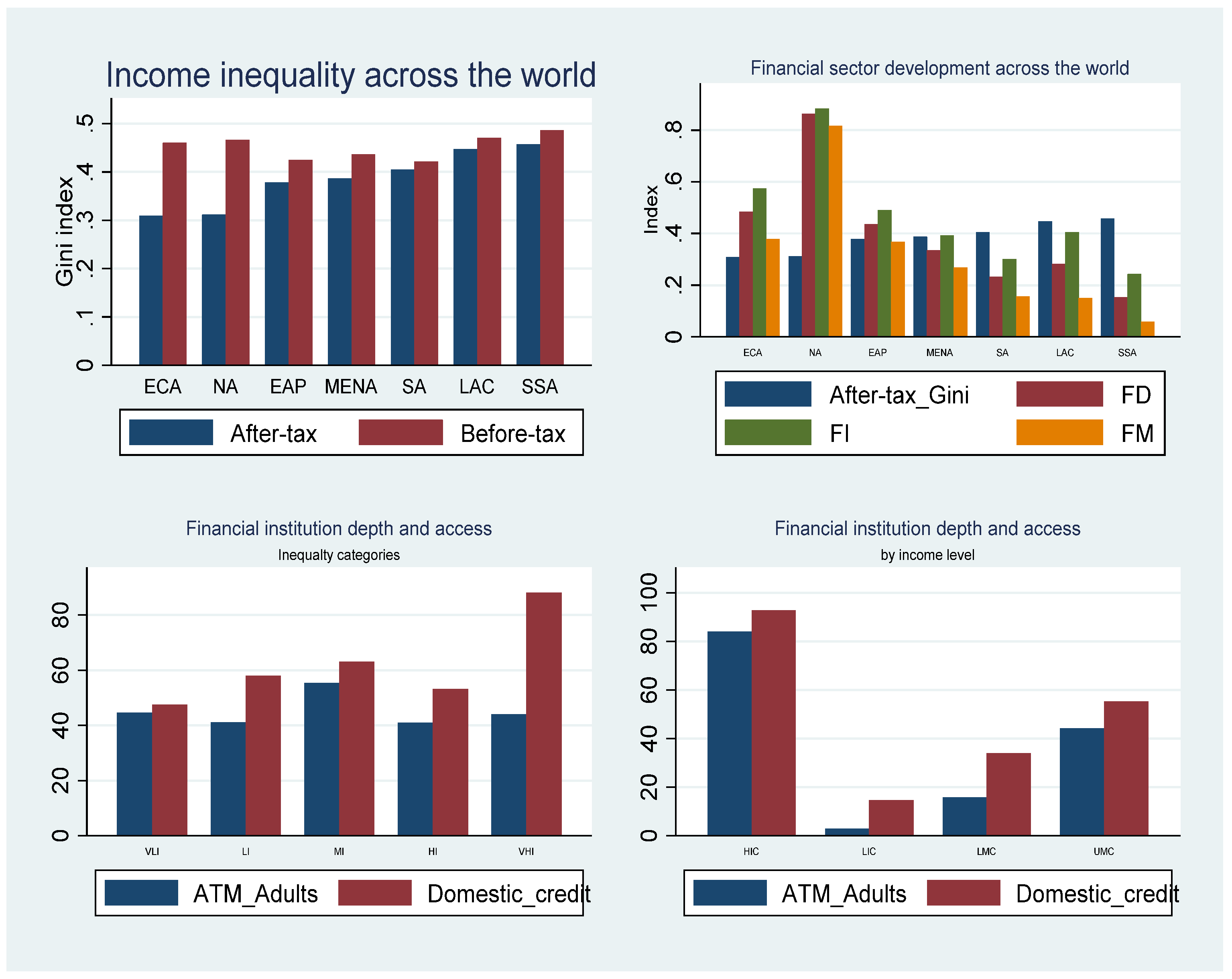
The top left graph shows global inequality levels in terms of both after-tax and before-tax Gini index by regions classified by the World Bank. Global income inequality data show that income inequality continues to rise within countries, while a comparison between countries shows that income inequality has declined on average. This is because inequality differs based on region. Regions such as Europe and Central Asia (ECA) have the lowest levels of income inequality. In contrast, sub-Saharan Africa (SSA) and Latin America and Caribbean (LAC) regions have rising and the highest levels of income inequality. For example, in the year 2016, the top 10% income group owned the national wealth of approximately 37% in Europe, 47% in the United States of America–Canada and 55% in sub-Saharan Africa, Brazil and India.

The top right graph shows the level of development in terms of financial sector (FD), financial institution (FI) and financial market (FM) indexes across the world. The North America (NA) region has the most developed financial sector, with all the FSD indexes above 0.80. The SSA, LAC and South Asia (SA) regions have the lowest overall FSD. On average, financial market development (FM) is significantly lower in SSA, LAC and SA regions. For example, South Africa has the most developed financial sector in the SSA region, with other countries depending on it.

The bottom left graph presents the level of financial institution depth (domestic credit) versus access (ATM per 100,000) based on income inequality categories. Countries with very low inequality (VLI) have higher levels of financial access than depth. Interestingly, domestic credit is much higher than access to financial services in very high-inequality countries. This suggests that higher domestic credit coupled with lower access to the financial sector are present in high-inequality countries. Lastly, the right bottom graph shows the level of financial institution depth versus access by income levels. From this figure, we can observe that higher levels of domestic credit by banks do not represent higher access to banking. High-income countries (HIC) have the highest level of both depth and access, while low-income countries (LIC) have the lowest of both. This suggests that FSD also depends on a country’s level of development (income level/region).

3. Methodology and Data

3.1. Methodology

The literature on FSD and income inequality lacks consensus, as shown above. The argument is that different measurements of FSD (mainly broader proxies), methodology and sample periods applied in the study can produce mixed results. This study contributes to the literature by investigating the impact of the overall FSD on income inequality and the impact of FSD dimensions (access and depth) on income inequality. This study is interested in testing both the linear and nonlinear relationship, as different stages of financial development can have different effects on income inequality. Empirical studies on the nonlinear relationship hypothesis suggest that measures of FSD be expressed in both linear and nonlinear forms (Greenwood and Jovanovic 1990). The system generalized method of moments (GMM) of Blundell and Bond (1998) and Roodman (2009) is applied. GMM estimation requires the time of data (t) to be smaller than the number of countries (i) in the panel data. GMM is a dynamic estimator used for panel data that uses instrumental variables and corrects for endogeneity. GMM is advantageous as it also controls omitted variable bias and controls for country fixed effect. The robust system GMM estimation technique provides the following diagnostic tests: the serial correlation AR(2), the Sargan test and the Hansen test, where the null hypothesis for the Sargan and Hansen test is that instruments are valid for the model. This study employs a robust system GMM which is an augmented estimator, where one equation is expressed in levels with instruments expressed in the first difference. In the GMM, I regressed the log of after-tax Gini index on its first lagged, whilst building orthogonal conditions in GMM addresses sources of endogeneities; see Gnangoin et al. (2019). In estimating all the GMM, corruption variables are entered as an exogenous instrumental variable. This variable serves as a proxy for institutional quality. Initial GDP per capita and first lagged after-tax Gini are used as endogenous instruments. The choice of instruments is guided by the literature—for example, (Park and Shin 2015; Sahay and Cihak 2020). The collapse instrument option applied in the GMM helps to reduce the number of instruments. Subsequently, all the estimated GMM results have a lesser number of instruments than the number of N. By using robust system GMM, the results report standard errors that are robust to heteroskedasticity and autocorrelation. Finally, the linear model and nonlinear model are estimated using Equations (2) and (3), respectively.

Giniit = α + β₀Gini_it-1 + β₁FSD_it + β₃X_it + ε_it

(2)

Giniit = α + β₀Gini_it-1 + β₁FSD_it + β₂FSD²_it + β₃X_it + ε_it

(3)

where i and t represent countries and time, respectively, while FSD represents the FSD dimensions investigated, X is a set of control variables, and ε is the error term.

3.2. Data

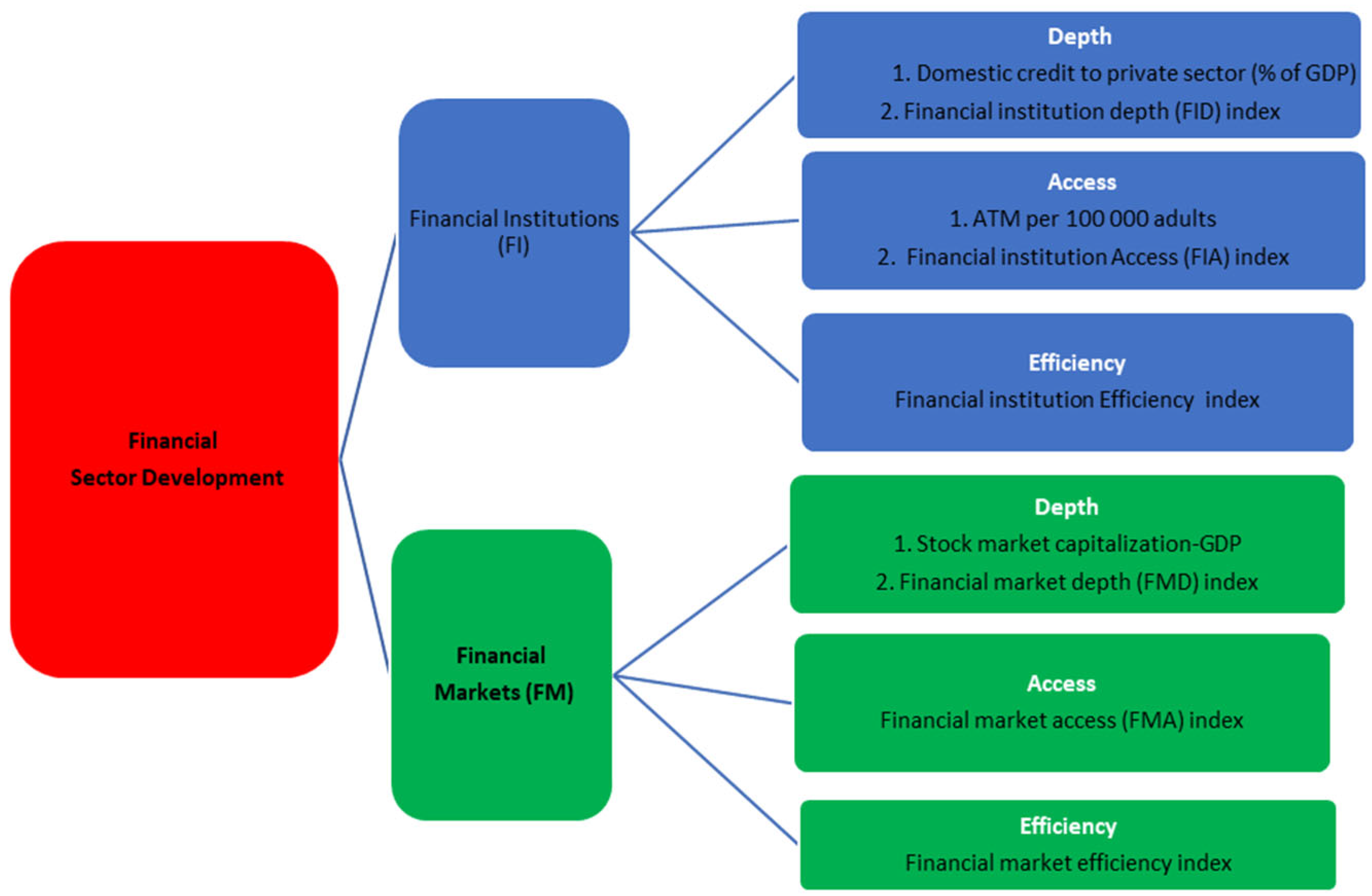
The concept of financial sector development (FSD) is compounded mainly in terms of structure and regulatory framework. However, we can decompose FSD first into two broad components: financial institutions (FI) and financial markets (FM). Financial institutions and markets are developed if they are characterized by increased depth, access, efficiency and stability. A large body of literature on FSD, income inequality and economic growth uses the depth of financial institutions or markets to measure FSD. Subsequently, there is a limited number of studies considering the multidimensions of FSD. After the year 2004, new data on the multidimensions of FSD emerged. Figure 2 below summarizes the multidimensions of FSD and only a selected few from the proxy variables for each category.

The panel data used in the study are sourced from different databases using Stata codes. This study employs yearly panel data of 120 countries (ccode) from the years 2004 to 2019, and the before- and after-tax Gini index from the Standardized World Income Inequality Database (SWIID). SWIID is one of the leading databases for global coverage inequality. Access to the financial sector is measured with the financial institution and market access indexes and the number of ATMs per 100,000 adults. The latter measure is one of the two financial access indicators for the UN 2030 SDGs target 8.10. For the control variables, average school years in the population aged 25 and older is the proxy for the education variable; GDP per capita and trade openness (Trade_op) were sourced from Pen World Tables (PWT). The World Development Indicator (WDI) of the World Bank provides the FSD measures, inflation rate and general government final consumption expenditure as a percentage of GDP(Gov). The consumer price index (CPI) is calculated using inflation data, where the year 2004 is the base year. The financial development indexes and ATM per 100,000 adults were sourced from the International Monetary Fund (IMF) database. The control for corruption variable reflects the ‘perception of the extent to which public power is exercised for private gain, including both petty and grand forms of corruption, as well as “capture” of the state by elites and private interests’ (Kaufmann et al. 2010). The corruption variable is sourced from the Worldwide Governance Indicator (WGI) of the World Bank. A detailed summary statistic is given in

Table A2. Descriptive Statistics.

Variable	Obs	Mean	Std. Dev.	Min	Max	Data Source
gini disp	1962	0.386	0.082	0.23	0.674	SWIID
gini mkt	1962	0.459	0.065	0.219	0.725	SWIID
GDP	2272	1.885	2.036	0.025	16.652	PWT
ATMadult	2110	0.46	0.459	0	2.886	IMF
Dom credit	2309	0.568	0.465	0	3.046	WDI
Fin markets	1034	0.727	1.311	0	13.496	WDI
FD	2320	0.336	0.236	0.029	1	IMF
FIA	2320	0.36	0.277	0.003	1	IMF
FMA	2320	0.241	0.288	0	1	IMF
FID	2320	0.279	0.271	0	1	IMF
FMD	2320	0.245	0.287	0	1	IMF
Urban pop	2320	0.578	0.23	0.091	1	WDI
Trade op	2272	0.645	0.565	0.001	5.49	PWT
yr sch	2016	8.242	3.342	0.759	15.802	PWT
CPI	2240	1.662	1.16	0.99	25.777	WDI
Gov	2127	0.157	0.053	0.035	0.435	WDI
corruption	2320	0.018	1.012	−1.681	2.47	WGI

of Appendix A. FSD indicators are chosen based on the available limited sample coverage in the panel setup, whilst trying to incorporate other proxy variables which are under test in the empirical literature.

4. Results

This section presents the linear and nonlinear empirical model results on the impacts of financial sector development (FSD) on inequality. Thus, this section presents results on the impact of overall FSD on income inequality, where overall FSD represents the development of both institutions and the market in terms of efficiency, depth and access. This study is interested in also investigating the impacts of FSD components on income inequality. Thus, the overall impact of financial institution (i.e., banks) and market (i.e., stock market) development is considered on income inequality. Thereafter, results on the impact of FSD in two dimensions (access and depth) on income inequality are presented. Financial sector depth (trade volumes and credit) is fundamentally different from access to financial services.

Table 2. Impact of overall financial sector development on income inequality.

	(1)	(2)	(3)
	Financial Development Index	Financial Institution Index	Financial Market Index
VARIABLES
L.log_gini_	0.710 ***	0.735 ***	0.726 ***
	(0.125)	(0.105)	(0.121)
Findev	−0.0644 **	−0.0615 *	−0.0434 **
	(0.0261)	(0.0353)	(0.0187)
GDP	0.00417	0.00295	0.00488
	(0.00377)	(0.00347)	(0.00380)
Log_cpi	0.0106	0.0133	0.00930
	(0.00872)	(0.00820)	(0.00827)
Trade_op	−0.00238	−0.00106	−0.00444
	(0.00706)	(0.00733)	(0.00700)
Log_Gov	0.00769	0.0113	0.00262
	(0.0188)	(0.0204)	(0.0180)
Log_Education	−0.0913	−0.0803	−0.0977 *
	(0.0582)	(0.0524)	(0.0580)
Constant	−0.0728	−0.0590	−0.0647
	(0.0810)	(0.0774)	(0.0794)
Observations	1508	1508	1508
Number of ccode	120	120	120
AR 2 test (p-value)	0.558	0.396	0.529
Sargan test (p-value)	0.995	0.943	0.305
Hansen test(p-value)	0.270	0.308	0.202

Robust standard errors in parentheses. *** p < 0.01, ** p < 0.05, * p < 0.1.

reports the results of the linear model (Equation (2)) on the impact of overall FSD on income inequality. The dependent variable is the log of the after-tax Gini index. This is because the after-tax Gini index is an important measure of income inequality, as progressive tax policies are praised for reducing income inequality. In line with the growing and large literature, all three models confirm an overall narrowing impact of FSD on income inequality. These results are consistent with the results of Nguyen et al. (2019). The coefficients of the FSD index and financial market index (model 1 and 3, respectively) are negative and significant at 5%, while the narrowing hypothesis is confirmed only at 10% in the overall development of financial institutions (model 2). Table 2 results suggest that overall FSD reduces inequality with a range of 4 to 6%. The nonlinear results of the overall impact of FSD on income inequality were not significant, and are thus not reported in the study.

Table 3. Impact of access to financial institutions and markets on income inequality.

	(1)	(2)	(3)	(4)	(5)	(6)
	Financial Institution Access Index	ATM per 100,000 Adults	Financial Market Access Index	Financial Institution Access Index	ATM per 100,000 Adults	Financial Market Access Index
VARIABLES
L.log_gini	0.754 ***	0.801 ***	0.812 ***	0.744 ***	0.794 ***	0.853 ***
	(0.118)	(0.0852)	(0.0832)	(0.126)	(0.0834)	(0.0785)
Financial Access	−0.0542 **	−0.0278 *	0.00810	−0.0270	−0.0647 **	0.158
	(0.0234)	(0.0145)	(0.00985)	(0.107)	(0.0316)	(0.100)
Financial Access2				−0.0280	0.0216	−0.123
				(0.100)	(0.0161)	(0.0850)
GDP	0.00144	0.00473	0.00363	0.00208	0.00159	0.00209
	(0.00355)	(0.00341)	(0.00290)	(0.00372)	(0.00277)	(0.00276)
Log_CPI	0.0183 *	0.0205 **	0.0131 *	0.0182	0.0221 **	0.0172 **
	(0.0103)	(0.00875)	(0.00688)	(0.0110)	(0.00846)	(0.00808)
Trade_op	0.00801	0.000966	−0.00462	0.00783	0.00383	−0.00766
	(0.00719)	(0.00660)	(0.00600)	(0.00753)	(0.00690)	(0.00674)
Log_Gov	0.0253	0.0217	0.00193	0.0265	0.0185	−0.00747
	(0.0227)	(0.0201)	(0.0165)	(0.0221)	(0.0200)	(0.0160)
Log_Education	−0.0883	−0.0891 *	−0.0892 **	−0.0988	−0.0652 *	−0.0891 **
	(0.0542)	(0.0484)	(0.0433)	(0.0608)	(0.0367)	(0.0429)
Constant	−0.00868	0.0233	−0.0131	−0.000560	−0.0270	−0.00933
	(0.0882)	(0.0854)	(0.0722)	(0.0877)	(0.0851)	(0.0721)
Observations	1508	1416	1508	1508	1416	1508
Number of ccode	120	119	120	120	119	120
AR 2 test (p-value)	0.498	0.211	0.339	0.643	0.226	0.361
Sargan test (p-value)	0.994	0.908	0.729	0.995	0.952	0.898
Hansen test (p-value)	0.656	0.644	0.250	0.613	0.587	0.366

Robust standard errors in parentheses. *** p < 0.01, ** p < 0.05, * p < 0.1.

presents the results of the linear model (model 1, 2, 3) and nonlinear model (model 4–6) on the impact of access to financial services on income inequality. The dependent variable is the log of the after-tax Gini index. The result from both the linear and nonlinear model confirms that access to financial institution services has a significant reducing impact on income inequality (models 1, 2, 5). Increased access to financial institutions also reduces income inequality by promoting informal sector participation in the real economy. However, the model of access to the financial market (model 3, 6) shows that there is not a significant relationship with income inequality.

Table 4. Impact of financial institution and market depth on income inequality.

	(1)	(2)	(3)	(4)	(5)	(6)
	Domestic Credit % of GDP	Financial Institution Depth Index	Financial Market Depth Index	Domestic Credit % of GDP	Financial Institution Depth Index	Financial Market Depth Index
VARIABLES
L.log_gini	0.763 ***	0.821 ***	0.782 ***	0.764 ***	0.761 ***	0.774 ***
	(0.120)	(0.0661)	(0.0890)	(0.118)	(0.0813)	(0.0884)
Financial depth	−0.0221 **	0.0198	−0.0100	−0.0294	−0.232 **	−0.0329
	(0.0110)	(0.0350)	(0.0114)	(0.0356)	(0.103)	(0.0298)
Financial depth2				0.00364	0.185 **	0.0215
				(0.0175)	(0.0843)	(0.0259)
GDP	0.00540	0.00340	0.00395	0.00535	0.000844	0.00383
	(0.00422)	(0.00273)	(0.00306)	(0.00427)	(0.00285)	(0.00313)
Log_CPI	0.0157	0.0137	0.0116	0.0158	0.00804	0.0113
	(0.00977)	(0.00837)	(0.00733)	(0.00962)	(0.00772)	(0.00746)
Trade_op	0.00109	−0.00465	−0.00630	0.00134	0.000720	−0.00609
	(0.00769)	(0.00561)	(0.00655)	(0.00819)	(0.00620)	(0.00664)
Log_Gov	0.0259	−0.00246	0.00160	0.0267	0.00837	0.00132
	(0.0225)	(0.0182)	(0.0169)	(0.0214)	(0.0196)	(0.0169)
Log_Education	−0.111 *	−0.0929 *	−0.0882 *	−0.110 *	−0.0411	−0.0873 *
	(0.0612)	(0.0485)	(0.0461)	(0.0643)	(0.0479)	(0.0467)
Constant	0.0377	−0.00852	−0.0388	0.0385	−0.101	−0.0454
	(0.101)	(0.0758)	(0.0739)	(0.0971)	(0.0751)	(0.0728)
Observations	1465	1508	1508	1465	1508	1508
Number of ccode	119	120	120	119	120	120
AR 2 test (p-value)	0.769	0.281	0.355	0.712	0.185	0.385
Sargan test (p-value)	0.997	0.726	0.822	0.994	0.923	0.805
Hansen test(p-value)	0.450	0.275	0.177	0.413	0.224	0.218

Robust standard errors in parentheses. *** p < 0.01, ** p < 0.05, * p < 0.1.

presents the results of the linear model (model 1, 2, 3) and nonlinear model (model 4–6) on the impact of the financial institution and market depth on income inequality. The dependent variable is the log of the after-tax Gini index. As with the findings on financial market access in Table 3, Table 4 also suggests that financial market depth has no significant impact on income inequality. From Table 4, we can infer that in the linear models, only domestic credit by banks (model 1) is negative and significant at a 5% level. The study finds that the Too Much Finance hypothesis holds. In other words, in the nonlinear models, the financial institution depth index (model 5) confirms a U-shaped relationship with income inequality. The U-shaped finance depth and income inequality relationship suggests that increasing depth first narrows income inequality and, after reaching a threshold, growth in depth produces widening effects on income inequality. Thus, excessive credit could widen income inequality.

All the GMM results in Table 2, Table 3 and Table 4 above present the GMM diagnostic test results in the last three rows, where all the models showed no evidence of serial correlation, as indicated by the Arellano–Bond test for serial correlation (AR2). The Sargan and Hansen test investigates the validity of the chosen instruments of the model. The Sargan test of overidentifying restrictions is a special case of the Hansen test, as it assumes homoskedasticity and no serial correlation in the error terms, while the Hansen test does not rely on these strong assumptions (Roodman 2007). The Hansen test of overidentifying restrictions depends on the estimate of an optimal or robust weighting matrix, while the Sargan test does not (Roodman 2007). Thus, the Hansen and Sargan test results have different p-values. The p-values for both Sargan and Hansen tests in all the above results are above 10%, suggesting that, under both assumptions on error terms, the model instruments are valid. For robust standard errors, this study places emphasis on the Hansen test on instrument validity, while noting that Hansen test p-values below 0.25 should be viewed with caution (for example, model 3 of Table 2; model 3, 5 and 6 of Table 4) (Roodman 2007). However, the debate in the literature regarding the p-values of the Hansen test and the number of instruments in GMM continues; hence, this study also uses the collapse option to ensure that the number of instruments does not produce bias in the test of instrument validity (Roodman 2007).

5. Discussion

This study investigated the impact of overall FSD, and two dimensions of FSD, on income inequality. As such, the discussion is threefold, as follows.

Overall Impact of FSD on Income Inequality

The results presented in Table 2 contribute to the literature by providing an overall effect of FSD on income inequality. Few studies have empirically tested the impact of overall FSD on income inequality (Nguyen et al. 2019). The study of Nguyen et al. (2019), confirms an inverted U-shaped relationship between the FSD index of IMF and income inequality in emerging market countries. According to my knowledge, there are no studies empirically testing the impacts of the overall financial institution and market indexes on income inequality. Rather, what is common in the literature is studies using mostly financial depth to proxy overall FSD.

Impact of Financial Access on Income Inequality

The models of access to financial institution services (Table 3) confirm a narrowing impact on income inequality. These results are in line with the literature arguing for increased access to reduce income inequality (Kapingura 2017; Hasan et al. 2020; Sahay and Cihak 2020). For instance, Sahay and Cihak (2020) utilized three methods including Arellano and Bond (1991) GMM and confirmed the narrowing impact of financial access to income inequality on the five-year non-overlapping data of 128 economies and in a sub-group of emerging markets and developing countries. Sahay and Cihak (2020) and Hasan et al. (2020) both proxied financial access by the number of ATMs and commercial banks per 100,000 adults, while this study adds to the literature on financial access and income inequality by including results from the financial institution access index. Thus, this paper adds consensus on the effect of the access dimension of FSD on income inequality. Lastly, in Table 3, the linear model suggests that access to the financial market increases income inequality, while the nonlinear model suggests an inverted U-shaped relation. However, the models of financial market access to income inequality were both insignificant. Intuitively, having access to the financial market seems to have no significant impact on income inequality. For instance, average-income households with little or no savings will not participate in the financial market even if they have access to them. This suggests that participation especially in the financial market is highly connected to an individual’s wealth and education. Access to financial institutions allows households of any income level to be able to build banking relations and credit scores.

Impact of Financial Depth on Income Inequality

In terms of financial institution depth (Table 4), the study first confirms a narrowing hypothesis on income inequality in the linear model—only when depth is measured as domestic credit as a share of the GDP. The impact of financial market depth on income inequality was insignificant in both the linear and nonlinear model. The insignificant results suggest that financial market depth maybe has a direct relation with inequalities of wealth, rather than income. This is because financial market development tends to widen wealth inequalities as compared to income. For example, the findings of Eurofound (2021) suggest that homeownership increases the bottom quintile wealth levels, and there are a relatively lower number of renters holding financial assets beyond deposits within the EU member state. At the same time, the wealthiest groups in the EU member state tend to earn income from a self-employed business, holding financial assets and real estate. This distribution of capital suggests that different income groups benefit differently from financial rent. While the linear results of the financial institution depth index were not significant, they become significant after adding the nonlinear term. Furthermore, the nonlinear model results from the financial institution depth index reveal that the Too Much Finance hypothesis is evident, thus suggesting a U-shaped relationship between financial depth and income inequality. The U-shaped relationship on finance depth and income inequality was also confirmed in the literature (Brei et al. 2018; Sahay and Cihak 2020; and de la Cuesta-González et al. 2020). For instance, Sahay and Cihak (2020) confirm the U-shaped finance depth and inequality nexus using financial institution and market depth. de la Cuesta-González et al. (2020) confirm the U-shaped hypothesis using both domestic credits as a share of GDP and stock market capitalization on the income inequality of nine OECD countries, using a two-step GMM. The widening effect of higher credit on inequality is explained by how credit is highly dependent on collateral, firm structure and sector of activity. Bank credit decisions can have a negative or positive influence on an individual’s future income. According to Delis et al. (2021), in 5 years, individuals who are accepted for loan applications can grow their future income by 11% versus those who were rejected. For example, an individual accepted for a mortgage loan will have a higher net worth than those rejected. A firm receiving a loan for investment tends to be more profitable than those rejected for loans. These firms are expected to develop and implement certain rules as per the loan agreement. The growth of these firms with accepted loans produces increases in their wages, thus widening income inequality as the wages and productivity of the firms who were declined credit do not increase. Thus, income distribution is much tighter among accepted loan applications versus the wider distribution seen on a rejected loan application.

In addition, when the credit market triggers speculative investment, domestic credit increases income inequality in Vietnam (Le and Nguyen 2020). Financial policies focusing on alleviating income inequality should also incorporate credit policy provisions, whilst reviewing the banking business model to safeguard credit distribution in the direction of inclusive growth and sustainable development (de la Cuesta-González et al. 2020). The widening impact of domestic credit on inequality can also be reduced through policy interventions to increase access to credit efficiently. For example, the European Bank for Reconstruction and Development (EBRD) provides credit to individuals, firms and SMEs that are credit-constrained but have good investment plans or good business financials.

6. Conclusions

The literature on income inequality and financial sector development (FSD) is dense, with extensive studies using broader measures of FSD. This study adds to the literature by looking first at the overall impact of FSD on income inequality using the FSD index, as done by Nguyen et al. (2019), whilst also investigating individually the impact of financial market and institution development on income inequality. This study also investigates the multidimensional perspective of FSD on income inequality. More specifically, this paper investigates the impact of financial sector depth (domestic credit) and access on income inequality. I used panel data of 120 countries from 2004 to 2019 and estimated the system GMM. The empirical results show a negative overall impact of FSD on income inequality. Furthermore, this study finds that access to financial institutions tends to narrow income inequality in both linear and nonlinear models. The narrowing hypothesis of financial access on inequality is evident in the literature, especially in the case of India, where the national bank used a policy mandate to broaden access to finance in rural areas. This includes poor households in the formal economy, allowing them to save and invest; it gives informal workers such as street vendors in Africa an opportunity to bank their income and thus start building credit for future loans. As such, access to financial institution services is the most important component of FSD when it comes to income inequality. However, both financial market access and depth seemed not to impact income inequality.

Contrary to financial access results, the empirical results on financial depth and income inequality were twofold. Firstly, in the linear model, financial depth as measured by domestic credit narrows income inequality. Secondly, only in the nonlinear financial depth index model, the study confirms a U-shaped relationship, suggesting that the Too Much Finance hypothesis holds. The U-shaped finance depth and inequality hypothesis implies that financial depth narrows income inequality up until a certain threshold, beyond which growth in financial depth widens income inequality. The findings of this study point towards incorporating inclusive FSD, by targeting inclusive credit policies and increasing access to financial services to reduce income inequality. This study does not disregard the other factors driving income inequality, such as wages (skills/education); however, the study points out other measures that can be taken to tackle inequalities. Exclusion from the financial sector reflects exclusion from the formal economy. While Fintech and other digital means of financial transaction are growing in Africa and India, this study leaves the analysis for future research.

References

- Arellano, Manuel, and Stephen Bond. 1991. Some Tests of Specification for Panel Data: Monte Carlo Evidence and an Application to Employment Equations. Review of Economic Studies 58: 277–97. [Google Scholar] [CrossRef] [Green Version]
- Banerjee, Abhijit V., and Andrew F. Newman. 1993. Occupational Choice and Process of Development. Journal of Political Economy 101: 274–98. [Google Scholar] [CrossRef]
- Batuo, Michael Enowbi, Francesco Guidi, and Kupukile Mlambo. 2010. Financial Development and Income Inequality: Evidence from African Countries. MPRA Paper 25658. Munich: University Library of Munich. [Google Scholar]
- Beck, Thorsten, Asli Demirguc-Kunt, and Ross Levine. 2004. Finance, Inequality, and Poverty: Cross-Country Evidence. NBER Working Papers 10979. Cambridge: National Bureau of Economic Research, Inc. [Google Scholar]
- Bittencourt, Manoel. 2011. Financial Development and Economic Growth in Latin America: Is Schumpeter Right? In Proceedings of the German Development Economics Conference. Berlin: Verein für Socialpolitik, Research Committee Development Economics. [Google Scholar]
- Bittencourt, Manoel, Shinhye Chang, Rangan Gupta, and Stephen Miller. 2019. Does Financial Development Affect Income Inequality in the US States? Journal of Policy Modeling 41: 1043–56. [Google Scholar] [CrossRef]
- Blundell, Richard, and Stephen Bond. 1998. Initial conditions and moment restrictions in dynamic panel data models. Journal of Econometrics 87: 115–43. [Google Scholar] [CrossRef] [Green Version]
- Brei, Michael, Giovanni Ferri, and Leonardo Gambacorta. 2018. Financial Structure and Income Inequality. BIS Working Papers 756. Basel: Bank for International Settlements. [Google Scholar]
- Burgess, Robin, and Rohini Pande. 2005. Do Rural Banks Matter? Evidence from Indian Social Banking Experiemnt. American Economic Review 95: 780–95. [Google Scholar] [CrossRef] [Green Version]
- Chiu, YiBin, and Chien-Chiang Lee. 2019. Financial development, income inequality, and country risk. Journal of International Money and Finance 93: 1–18. [Google Scholar] [CrossRef]
- Cihak, Martin, and Ratna Sahay. 2020. Finance and Inequality. IMF Staff Discussion Notes 2020/001. Washington, DC: International Monetary Fund. [Google Scholar]
- Clarke, George R., Lixin Colin Xu, and Heng-fu Zou. 2006. Finance and Income Inequality: What Do the Data Tell Us? Southern Economic Journal 72: 578–96. [Google Scholar]
- Dabla-Norris, Era, Kalpana Kochhar, Nujin Suphaphiphat, Frantisek Ricka, and Evridki Tsounta. 2015. Causes and Consequences of Income Inequality: A Global Perspective. IMF Staff Discussion Note 2015/013. Washington, DC: International Monetary Fund. [Google Scholar]
- de Haan, Jakob, and Egbert Sturm. 2017. Finance and income inequality: A review and new evidence. European Journal of Political Economy 50: 171–95. [Google Scholar] [CrossRef] [Green Version]
- de la Cuesta-González, Marta, Cristina Ruza, and José M. Rodríguez-Fernández. 2020. Rethinking the income inequality and financial development nexus. A study of nine OECD countries. Sustainability 12: 5449. [Google Scholar] [CrossRef]
- Delis, Manthos D., Fulvia Fringuellotti, and Steven R. G. Ongena. 2021. Credit, Income, and Inequality. FRB of New York Staff Report No. 929, Proceedings of Paris December 2020 Finance Meeting EUROFIDAI—ESSEC. Available online: https://ssrn.com/abstract=3631252 (accessed on 1 January 2022).
- Demirguc-Kunt, Asli, and Ross Levine. 2009. Finance and Inequality: Theory and Evidence. Annual Review of Financial Economics 1: 287–318. [Google Scholar] [CrossRef] [Green Version]
- Denk, Oliver. 2015. Financial Sector Pay and Labour Market Income Inequality: Evidence from Europe. OECD Economic Department Working paper 1225. Paris: OECD. [Google Scholar]
- Dollar, David, and Aart Kraay. 2002. Growth is Good for the Poor. Journal of Economic Growth 7: 195–25. [Google Scholar] [CrossRef]
- Ductor, Lorenzo, and Daryna Grechyna. 2015. Financial development, real sector, and economic growth. International Review of Economics & Finance 37: 393–405. [Google Scholar]
- Emrah, Koçak, and Uzay Nısfet. 2019. The effect of financial development on income inequality in Turkey: An estimate of the Greenwood-Jovanovic hypothesis. Review of Economic Perspectives 19: 319–44. [Google Scholar]
- Eurofound. 2021. Wealth Distribution and Social Mobility. Luxembourg: Publication Office of the European Union. [Google Scholar]
- Francese, Maura, and Carlos Mulas-Granados. 2015. Functional Income Distribution and Its Role in Explaining Inequality. IMF Working papers 2015/244. Washington, DC: International Monetary Fund. [Google Scholar]
- Galor, Oded, and Joseph Zeira. 1993. Income distribution and macroeconomics. Review of Economic Studies 60: 35–52. [Google Scholar] [CrossRef] [Green Version]
- Gnangoin, Yobouet Thierry Bienvenu, Liangsheng Du, GuyRoland Assamoi, Akadje JeanRoland Edjoukou, and Diby François Kassi. 2019. Public spending, income inequality and economic growth in Asian countries: A panel GMM approach. Economies 7: 115. [Google Scholar] [CrossRef] [Green Version]
- Goldsmith, Raymond William. 1969. Financial Structure and Development. New Haven: Yale University Press. [Google Scholar]
- Greenwood, Jeremy, and Boyan Jovanovic. 1990. Financial Development, Growth and distribution of income. Journal of Political Economy 98: 1076–107. [Google Scholar] [CrossRef] [Green Version]
- Gründler, Klaus, and Jan Weitzel. 2013. The Financial Sector and Economic Growth in a Panel of Countrie. Wirtschaftswissenschaftliche Beiträge, No. 123. Würzburg: Bayerische Julius-Maximilians-Universität Würzburg, Lehrstuhl für Volkswirtschaftslehre, insbes. Wirtschaftsordnung und Sozialpolitik. [Google Scholar]
- Gural, Anastasiya, and Iryna Lomachynska. 2017. Fdi And Financial Development As Determinants Of Economic Growth For V4 Countries. Baltic Journal of Economic Studies 3: 59–64. [Google Scholar] [CrossRef] [Green Version]
- Hasan, Iftekhar, Roman Horvath, and Jan Mares. 2020. Finance and wealth inequality. Journal of International Money and Finance 108: 102161. [Google Scholar] [CrossRef] [Green Version]
- Hendel, Igal, Joel Shapiro, and Paul Willen. 2005. Educational opportunity and income inequality. Journal of Public Economics 89: 841–70. [Google Scholar] [CrossRef] [Green Version]
- Jaumotte, Florence, Subir Lall, and Chris Papageorgiou. 2013. Rising Income Inequality: Technology, or Trade and Financial Globalization? IMF Economic Review 61: 271–309. [Google Scholar] [CrossRef] [Green Version]
- Kapingura, Forget M. 2017. Financial Sector development and income inequality in South Africa. African Journal of Economic and Management Studies 8: 420–32. [Google Scholar] [CrossRef]
- Kaufmann, Daniel, Aart Kraay, and Massimo Mastruzzi. 2010. The Worldwide Governance Indicators: A Summary of Methodology, Data and Analytical Issues. World Bank Policy Research Working Paper No. 5430. Washington, DC: World Bank. [Google Scholar]
- Kim, Dong-Hyeon, and Shu-Chin Lin. 2011. Nonlinearity in the financial development income inequality nexus. Journal of Comparative Economics 39: 310–25. [Google Scholar] [CrossRef]
- Kuznets, Simon. 1955. Economic growth and Income Inequality. The American Economic Review 45: 1–28. [Google Scholar]
- Law, Siong-Hook, and Hui-Boon Tan. 2012. Nonlinear dynamics of the finance-inequality nexus in developing countries. The Journal of Economic Inequality 10: 551–63. [Google Scholar]
- Le, Quoc Hoi, and Bich Ngoc Nguyen. 2020. The impact of credit on income inequality in Vietnam. The Journal of Asian Finance, Economics and Business 5: 111–18. [Google Scholar] [CrossRef]
- Levine, Ross. 2004. Finance and Growth: Theory and Evidence. Nber working paper series 10766; Amsterdam: Elsevier. [Google Scholar]
- Liang, Zhicheng. 2008. Financial development and income inequality in rural China 1991–2000. In Understanding Inequality and Poverty in China. London: Palgrave Macmillan, pp. 72–88. [Google Scholar]
- Mihalyi, Peter, and Ivan Szelenyi. 2019. Rent-Seekers, Profits, Wages and Inequality. The Top 20%. London: Palgrave Macmillan. [Google Scholar]
- Nguyen, Cong Thang, Tan Ngoc Vu, Duc Hong Vo, and Dao Thi-Thieu Ha. 2019. Financial Development and Income Inequality in Emerging Markets: A New Approach. Journal of Risk and Financial Management 12: 173. [Google Scholar] [CrossRef] [Green Version]
- Oluitan, Roseline. 2012. Financial Development and Economic Growth in Africa: Lessons and Prospects. Business and Economic Research 2: 54–67. [Google Scholar] [CrossRef]
- Ongena, Steven, and Lizethe Mendez-Heras. 2020. Finance and growth re-visited. Journal of Financial Management, Markets and Institutions 8: 2050001. [Google Scholar]
- Park, Donghyun, and Kwanho Shin. 2015. Economic Growth, Financial Development, and Income Inequality. ADB Economics Working Paper Series 441; Mandaluyong: Asian Development Bank. [Google Scholar]
- Paun, Cristian Valeriu, Vladimir Mihai Topan, and Radu Cristian Musetescu. 2019. The Impact of Financial Sector Development and Sophistication on Sustainable Economic Growth. Sustainability 11: 1713. [Google Scholar] [CrossRef] [Green Version]
- Piketty, Thomas. 2014. Capital in the Twenty-First Century. Cambridge: Belknap Press. [Google Scholar]
- Prete, Anna. 2013. Economy literacy, inequality, and financial development. Economics Letters 118: 74–76. [Google Scholar] [CrossRef] [Green Version]
- Rajan, Raghuran G., and Luigi Zingales. 2003. Saving Capitalism from the Capitalist. New York: Crown Business. [Google Scholar]
- Roodman, David. 2007. A Short Note on the Theme of Too Many Instruments. Working paper number 125. Washington, DC: Center for Global Development. [Google Scholar]
- Roodman, David. 2009. How to do xtabond2: An introduction to difference and system GMM in Stata. The Stata Journal 9: 86–136. [Google Scholar] [CrossRef] [Green Version]
- Sahay, Ratna, Martin Cihak, Papa M N’Diaye, Adolfo Barajas, Srobona Mitra, Annette J. Kyobe, Yen N. Mooi, and Reza Yousefi. 2015. Rethinking Financial Deepening; Stability and Growth in Emerging Markets. IMF Staff Discussion Notes 2015/008. Washington, DC: International Monetary Fund. [Google Scholar]
- Setiawan, Sigit. 2015. Financial depth and financial access in Indonesia. Journal of Indonesian Economy and Business 30: 139–58. [Google Scholar] [CrossRef] [Green Version]
- Seven, Unal, and Yener Coskun. 2016. Does financial development reduce income inequality and poverty? Evidence from emerging countries. Emerging Markets Review 26: 34–63. [Google Scholar] [CrossRef]
- Shahbaz, Muhammad, and Faridul Islam. 2011. Financial development and income inequality in Pakistan: An application of ARDL approach. Journal of Economic Development 36: 35–58. [Google Scholar] [CrossRef]
- Shahbaz, Muhammad, Nanthakumar Loganathan, Aviral Kumar Tiwari, and Reza Sherafatian-Jahromi. 2015. Financial Development and Income Inequality: Is There Any Financial Kuznets Curve in Iran? Social Indicators Research: An International and Interdisciplinary Journal for Quality-of-Life Measurement 124: 357–82. [Google Scholar] [CrossRef] [Green Version]
- Sunde, Tafirenyika. 2012. Financial Sector Development and Economic Growth Nexus in South Africa. MPRA Paper 86633. Munich: University Library of Munich. [Google Scholar]
- Svirydzenka, Katsiaryna. 2016. Introducing a New Broad-Based Index of Financial Development. IMF Working Papers 2016/005. Washington, DC: International Monetary Fund. [Google Scholar]
- Wahid, Abu NM, Muhammad Shahbaz, Mehmood Shah, and Mohammad Salahuddin. 2012. Does Financial Sector Development Increase Income Inequality? Some Econometric Evidence from Bangladesh. Indian Economic Review, Department of Economics, Delhi School of Economics 47: 89–107. [Google Scholar]
- Worku, Urgaia R. 2014. The Contribution of Financial Sector Development for Economic Growth in East Africa. Applied Economics and Finance 3: 201–14. [Google Scholar] [CrossRef] [Green Version]
- Younsi, Moheddine, and Marwa Bechtini. 2020. Economic Growth, Financial Development, and Income Inequality in BRICS Countries: Does Kuznets’ Inverted U-Shaped Curve Exist? Journal of the Knowledge Economy 11: 721–42. [Google Scholar] [CrossRef]
Figure 1.
Stylized facts.
Figure 2.
Measuring FSD. Source: Own processing based on Figure 1, on page 12 of Sahay et al. (2015), and Table 1 of Svirydzenka (2016).