Nonlinear Dynamics of the Development-Inequality Nexus in Emerging Countries: The Case of a Prudential Policy Regime

Abstract

This study analyses the nonlinear dynamic impact of economic development on income inequality in a prudential policy regime in a panel of 15 emerging markets from 1985–2019. More importantly, we seek to extend the existing debate on this subject, with roots back to the seminal work by Kuznets and many others, and add a twist by introducing a distinction between a prudential regime (1985–1999) and a non-prudential regime (2000–2019), as well as the threshold level at which economic development reduces inequality, using Panel Smooth Transition Regression (PSTR). The Generalized Method of Moments and fixed-effect models will be used to support our baseline results. The PSTR model was adopted due to its ability to deal with features that cannot be accounted for in dynamic panel techniques, such as endogeneity, homogeneity, cross-country variability, and time instability within the model. We found evidence of a non-linear effect between the two variables, where the threshold was found to be US$13,800, above which economic development reduces inequality in selected countries, and this further confirms the Kuznets inverted U-shape in both regimes. Macroprudential policies were found to trigger development-inequality relationships. Our evidence largely suggests that policymakers ought to formulate policies that aim to attract investment, which will then create job opportunities and foster an improvement in the stan-dard of living, and also should be abreast of the level of economic development before implementing macroprudential policies.

1. Introduction

The effect of economic development on income inequality has been a debated subject for the past decades. To date, there have been controversies in both the theoretical predictions and empirical literature in identifying the role played by economic development in income inequality. Theories, such as the Kuznets hypothesis, postulate that there is nonlinearity between economic development and income inequality, stating that inequality tends to escalate during the early phase of development, as labour migrates from the low-paying sector, agriculture, to the high-paying sector, urban and non-agricultural economic activities (Kuznets 1955). The Kaldor theory states that, if capitalists save more than workers, fast rates of growth are associated with a higher share of the profits (Kaldor 1955).

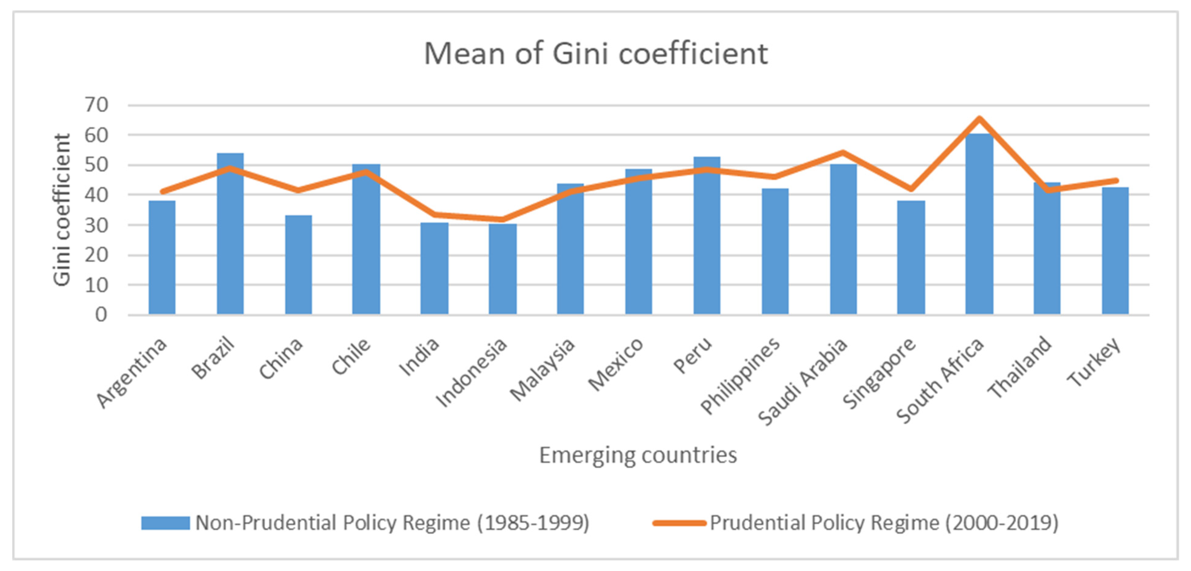
Figure 1 graphically demonstrates the mean Gini coefficient for both the prudential (1985–1999) and non-prudential policy regimes (2000–2019).

The insight gained from these two regimes (prudential and non-prudential policy regimes) demonstrates that during the non-prudential policy regime, about four countries, namely, Brazil, Chile, Malaysia, Mexico, Thailand, and Peru, experienced high income inequality as the Gini coefficient is above that of the prudential policy regime.

The remaining nine countries that are included in the sample are experiencing the challenge of high income inequality during the prudential policy regime, as the mean Gini coefficient is above the mean reported during the non-prudential policy regime.

The extant literature on the relationship between economic development and income inequality is vast and has capitulated extensive conflicting outcomes. Some authors found non-linearity, claiming that the relationship between economic development and income inequality is explained by the Kuznets inverted U-shape (Paukert 1973; Papanek and Kyn 1986; Jha 1996; Tirado et al. 2016), and others the U-shape (Savvides and Stengos 2000; Angeles 2010; Zungu et al. 2021). There are also authors who fail to support the Kuznets curve hypothesis (Robinson 1976; Anand and Kanbur 1993; Ram 1997; Deininger and Squire 1998; Tribble 1999; Theyson and Heller 2015; Kavya and Shijin 2020), while others find it inconclusive (Barro 2000), or a mixed relationship (Shahbaz 2010). The contradiction in these results may be due, but not limited to, the feasible explanation that the divergent results in the existing literature lie in the different model specifications, data sets, and estimation techniques, or the level of the economy being studied, when examining the development-inequality relationship.

This study extends the existing literature on this subject matter, following the seminal work of Kavya and Shijin (2020), who supported the Kuznets view by using panel GMM estimation tools on an unbalanced panel of 85 countries. In their analysis, they captured economic development, using the GDP per capita constant in 2010, while the Gini coefficient was used to capture income inequality. Their study controls for urban populations, inflation, trade, and government spending. Our study seeks to extend the existing debate on this subject matter, with roots back to the seminal work by Kuznets and many others on the so-called inverted U-shaped relationship, and then to add a twist by introducing a distinction between a prudential and a non-prudential regime, referring to the periods 1992–2005 and 2006–2019, respectively. Furthermore, we seek to include major monetary policy variables, known as macroprudential monetary policy instruments (such as borrower-related and capital-related instruments) that were adopted by federal banks in va- rious countries during the financial crisis of 2007. In a nutshell, we aim to examine how the adopted macroprudential policies during the financial crisis triggered the development-inequality relationship in emerging countries.

After reviewing the existing literature on the monetary policy side of the argument, these policies are argued to have a direct or indirect impact on inequality, which was not captured in the Kavya and Shijin (2020) model. We further believe that the correlation between the two variables might differ as countries switch from the non-prudential policy regime to a prudential policy regime. Furthermore, their study did not provide the threshold point above which economic development reduces inequality. Besides that, their ana-lysis was based on a group of countries with different levels of economic development.

It is because of these inconclusive and sometimes conflicting views that we seek to fill the gap in the literature by incorporating and examining the impact of economic development and those monetary policy variables and their effects on inequality in a group of emerging markets that most of the existing studies have not given attention to, and also by providing the threshold level of economic development that adversely affects inequality. This will provide new evidence in an emerging literature. We constructed a balanced panel of 15 emerging markets covering the period 1985–2019. Due to data availability, the non-prudential policy regime covers the period from 1985–1999, while the prudential regime starts with the period from 2000–2019. The 15 emerging countries are Singapore, Saudi Arabia, Chile, Turkey, Brazil, Mexico, Argentina, Malaysia, South Africa, Thailand, Peru, China, Indonesia, the Philippines, and India.

Specifically, this study proposes to clarify this debate by analysing the non-linear effects of economic development on inequality, employing the Panel Smooth Transition Regression (PSTR) model as well as the panel Generalized Method of Moments (GMM) and fixed-effect estimators. Furthermore, the PSTR model has never been applied to investigate this topic, despite the fact that it appears to be immensely relevant. This model definitely allows for an examination of the impact of economic development as shown by its various phases. The PSTR model could provide new insights, since this model endogenously identifies different regimes that correspond with distinct equations as well as the optimal degree of economic development, i.e., (id est/that is) the threshold value with respect to which the sign of the relationship could be different. Furthermore, the originality of the PSTR model consists of the fact that individuals can shift between groups and over time, as based on changes in the threshold variable. Because parameters fluctuate smoothly as functions of a threshold variable, the PSTR model also gives a parametric solution to the cross-country variability and time instability of the democracy-development coefficients. These features cannot be accounted for by dynamic or static panel techniques, nor by interaction effects. In addition, the time coverage of our panel data sets, compared to those in previous studies, makes our empirical model robust and useful for policy decision-making. Lastly, the inspiration for this study emanated not only from a lack of studies examining the non-linear effect of economic development on inequality in emerging economies, but more generally from the fact that this relationship may differ from the one that exists in the literature, due to the difference in the smoothness and implementation of their policies as well as the macro-economic policies that were adopted. Actually, our findings support the Kuznets inverted U-curve in both non-prudential and prudential policy regimes. However, what is interesting is that, during the adoption of these policies, they triggered the development-inequality relationship in emerging markets.

The remaining portion of the paper is organized as follows. Section 2 briefly surveys the related literature. Section 3 presents an overview of the model. Section 4 discusses the results of the PSTR, GMM, and FE models. Section 5 provides concluding remarks and discusses policy implications.

2. Literature Review

2.1. Theoretical Debate on Financial Growth

The Kuznets (1955) theory postulates that there is non-linearity between economic development and income inequality, stating that inequality tends to escalate during the early phase of development, as labour migrates from the low-paying sector, agriculture, to the high-paying sector, urban and non-agricultural economic activities. Thus, there are two stages of the evolution of the overall income distribution. The assumption made by Kuznets (1955) and the function that he specified is expressed as follows:

$$\mathrm{Gini}={\beta }_0+{\beta }_1\mathrm{ED}-{\beta }_2{\mathrm{ED}}^2+\mu ,$$

(1)

The Kuznets theory stresses two phases of the economy, the first phase being represented by the coefficient ${\beta }_1\mathrm{ED}$ (economic development), which emphasizes that, during the initial stage, economic development increases inequality as there will be an expansion of the weight of the non-agricultural sector. The second phase of the economy begins where the share of labour in the agricultural sector shrinks, a tipping point is eventually reached, and the inequality starts to decrease (given the very low weight of the agricultural and rural sector) as demonstrated by the coefficient ${\beta }_2{\mathrm{ED}}^2$ (economic development). For our study, following the Kuznets theory, we used GDP per capita as a proxy for economic development.

2.2. Empirical Review

2.2.1. Economic Development and Income Inequality

After reviewing the literature, it became clear that the relationship between economic development and income inequality seems to have received limited attention to date. However, to date, some economic questions have remained unanswered. The development-inequality nexus seems to have been ignored in the literature as, after scrutinizing the empirical literature on this subject matter, we were unable to find any recent literature except for the study by Kavya and Shijin (2020). This raises the concern whether this means that the development-inequality problem has been solved and is being well-understood? Looking at the inconsistent results in the existing literature, it necessitates conducting a new study that uses recent data and economic models.

Going as far back as Ahluwalia (1976), the development-inequality relationship was studied using cross-country data. The empirical findings failed to support the Kuznets hypothesis. However, the study by Ahluwalia (1976) contradicts the results reported by Robinson (1976), whose findings claim that the Kuznets hypothesis holds. After seven years, the argument was taken up again by Saith (1983) in a case of 60 countries, where six were socialist, 41 were developing and 13 were capitalist economies. Saith (1983) claims that studies, such as that of Ahluwalia (1976) and many others, were found to be based on defective statistics and questionable methodological premises. Papanek and Kyn (1986) studied the same subject using the panel data of 83 countries over the period 1952–1978 to test the validity of the Kuznets hypothesis. Their empirical findings support the Kuznets inverted U-shape, which then contradicts the findings reported by Ahluwalia (1976).

The findings by Papanek and Kyn (1986) were supported by Anand and Kanbur (1993) in a case of 60 developed and developing countries. Their empirical findings were further supported by Jha (1996), who studied the same subjects in the case of 76 countries over the period 1966–1992, using pool regression. In their model, different measures of income inequality, such as the share of the total income accruing to the poorest 20% of the population and the share of the total income accruing to 40% of the population, were adopted as a proxy for inequality. They claimed that the data used for inequality caused a severe problem that could have led to an incorrect conclusion and/or nullified the estimates.

After 44 years, the argument for the Kuznets hypothesis was a topic for debate (Barro 2000). Using panel data over the period 1965–1995, a panel analysis claim was made that the well-known Kuznets hypothesis did not fully explain the impact of economic deve-lopment on inequality over time. The result documented by Barro (2000), contradicted the findings reported by Papanek and Kyn (1986) and Jha (1996). In the same year, Savvides and Stengos (2000) tested the Kuznets hypothesis on a panel of 95 countries, using a threshold model. In their analysis, they adopted the data from Deininger-Squire. They found that the nature of the relationship between the two variables is U-shaped, which contradicts the Kuznets hypothesis. Nine years later, we observed the study by Angeles (2010), who studied the same subject in a case of 32 countries using a panel regression model. The main aim of the study was to assess the alternative test of the Kuznets hypothesis, using the Gini coefficient as a proxy for income inequality. The empirical findings supported the study by Savvides and Stengos (2000), claiming that the relationship between the two variables is a U-shaped relationship. The results by Barro (2000) were supported by Shahbaz (2010), using the ARDL bounds-testing approach to test the validity of the Kuznets hypothesis in time-series data over the 1971–2005 period in the case of Pakistan. The findings documented by Shahbaz (2010) are mixed, as they confirm the Kuznets inverted U-shape and the S-shape in Pakistan.

Theyson and Heller (2015) employed the panel fixed-effect technique to investigate the impact of economic development on income inequality in the case of 147 countries from 1992–2007. They pointed out that the Kuznets hypothesis failed to explain the whole process, claiming that the relationship is explained by an S-shape. Their finding contradicts those studies that claim the Kuznets hypothesis holds (Robinson 1976), but supports the studies of Barro (2000) and Shahbaz (2010). The impact of economic development on regional inequality was studied by Tirado et al. (2016) in Spain over the period 1860–2010. In their study, they used a novel dataset, spanning 150 years, to empirically test the Kuznets curve, as well as to analyse the relationship between economic development and income inequality before the Kuznets hypothesis. Their analysis was based on observing the pattern of income inequality from 1860 to 2010. Their findings confirmed the existence of the Kuznets hypothesis, with the data demonstrating that there were two major phases between 1860 and 1930 that showed an increase in regional income, accompanied by an improvement in economic development. Then, regional convergence followed until the 1980s.

Recently, Kavya and Shijin (2020) studied the impact of economic development on income inequality in a panel of 85 countries, where 16 were low-income, 28 were high-income, and 41 were middle-income countries over the 1984–2014 period, using a GMM model. The findings revealed that the Kuznets curve holds for high-income countries.

2.2.2. Macroprudential Policies and Income Inequality

This study is the first to examine the impact of macroprudential policies on the development-inequality relationship. Therefore, we briefly explain the empirical relationship between macroprudential policies and income inequality. The existing empirical literature on the distributional impact of macroprudential policies shows that an increase in the adoption of these policies increases income inequality. After scrutinizing the empirical literature on this subject matter, the researcher revealed five relevant empirical papers that examine the impact of macroprudential policies on inequality (Zinman 2010; Tzur-Ilan 2016; Frost and van Stralen 2018; Acharya et al. 2020; Carpantier et al. 2018). The study by Zinman (2010) investigated wealth and income inequality and the consumption effects of macroprudential measures in the case of the state of Oregon in the USA. The empirical evidence shows that macroprudential policies have a redistributive effect on wealth and income inequality. The argument was further developed by Tzur-Ilan (2016) following a borrower-related argument using a macro-analytical framework to examine the introduction effect of the loan-to-value (LTV) limit in Israel. The empirical findings show that consumer credit is a form of unsecured debt associated with higher rates. Borrowers increase the economy’s overall exposure to the risk of recession and unemployment. The results support the argument that LTV macroprudential instruments are likely to make less-wealthy borrowers more vulnerable.

Furthermore, Acharya et al. (2020) studied the effect on residential mortgage credit of the introduction of DTI and LTV caps in Ireland. The results of this study support the argument that borrower-related macroprudential instruments make the wealthy group wealthier, thus increasing wealth inequality. Frost and van Stralen (2018) used the database of Cerutti et al. (2017) for 69 countries over the time span 2000–2013 to investigate the causal relationship between macroprudential instruments and the Gini coefficients of net and market inequality. The findings reveal evidence for the redistributive effects of macroprudential policy. Precisely, the findings show that tighter measures such as higher reserve requirements, LTV caps, as well as concentration and interbank exposure limits, increase income inequality. Carpantier et al. (2018) used a household survey for 12 European Area countries employing HFCS data. The author finds that caps on LVT ratios may reduce wealth inequality in the sense that households find it tougher to get a mortgage, which results in low indebtedness by pushing wealth inequality lower.

Konstantinou et al. (2021) investigated the impact of macroprudential policies and income inequality in former transition economies. Their results indicate that, in general, the adoption of these policies exacerbates income inequality. The effect, however, is contingent on the extent of the degree of financial development and globalization; low levels of openness and financial development exacerbate inequality. However, some macroprudential measures may result in lower income inequality, provided the adopting economy is sufficiently open and has a developed or unrestricted financial system.

3. Research Methods and Data Adopted for This Study

This study adopted data covering the period from 1985 to 2019. However, as the study aimed to investigate the non-linear dynamics of development inequality in a prudential policy regime in emerging markets, a non-prudential policy regime (1985–1999) and a prudential policy regime (2000–2019) were adopted. The time span of our study is divided following the Cerutti data (Cerutti et al. 2017). The Cerutti data included dummy-type variables for the implementation of various macroprudential instruments. We define the period of the prudential policy regime starting from 2000 onwards due to the availability of data starting from 2000 onwards, while from 1999 backwards is classified as the period of the non-prudential policy regime. Variables that were suggested in the literature as explaining the relationship between economic development and income inequality were utilized. The Gini coefficient was used as a proxy for income inequality (Gini) and GDP per capita in constant prices (US$) (ED) as a proxy for economic development. We then controlled for borrower-related (BOR) and capital-related instruments (CCC), government expenditure (GE), investments (INV), and house prices (HP).

In our model, we adopted borrower-related and capital instruments, where the borrower-related instrument is calculated by summing the loan-to-value ratio with the debt-to-income ratio, while for capital instruments we used the general counter-cyclical capital buffer requirement (CTC) as a measure. A simulation of the countercyclical capital buffer designed in the Basel III package could impact bank lending as the buffer could help to reduce credit growth during booms and attenuate the credit contraction once it is released. This would help to dampen procyclicality, in addition to the beneficial effects of higher capital levels in terms of higher banking sector resilience to shocks. Then, this might have a direct or indirect impact on income inequality. Following Acharya et al. (2020), who argued that the borrower-related macroprudential instruments make the wealthy group wealthier, thus increasing income and wealth inequality, we then wanted to empirically test whether the borrower-related instrument has a direct or indirect impact on the development-inequality relationship.

The aim was to capture the impact of these instruments on income inequality while government expenditure was adopted, given the fact that the government is used as a tool to trigger output, which then leads to high growth and high employment while simultaneously decreasing inequality. Based on the argument of production, investment is included because increased capital investment requires some goods to be produced that are not immediately consumed, but instead are used to produce other goods, such as capital goods that lead to an increase in economic growth, which will then decrease inequality. Lastly, house prices were adopted for two reasons: (1) the existing literature studied the impact of house prices on income inequality, documenting that increasing house prices resulted in a housing affordability crisis in various countries, and (2) house prices at the same time increased homeowners’ wealth.

For the robustness model, we adopted the Gini coefficient from WIIDv2c to measure income inequality. However, the data from WIIDv2c had the problem of missing values. We then applied the data interpolation system using Eviews9 to fill the missing gaps. The variables were extracted from SWIID (Solt 2020), WDI (2021) and Cerutti data (Cerutti et al. 2017).

Panel Smooth Transition Regression Model

To evaluate the non-linear dynamic effect of the development-inequality relationship, the PSTR model developed by González et al. (2017) was used. The simplest case of the PSTR model, with two extreme regimes in a single transition function for illustrating the threshold effect of economic development (${\mathrm{ED}}_{it},$) on income inequality (${\mathrm{Gini}}_{it}),$ is the following: Please unify the format. (Gini)

$${\mathrm{Gini}}_{it}={\mu }_i+{\lambda }_t+{\beta }_0{\mathrm{ED}}_{it}+{\beta }_1{\mathrm{ED}}_{it}\times g\left({\mathrm{q}}_{it};\gamma ,c\right)+{\beta }_2{Z}_{it}+u_{it}$$

(2)

where $i=1,\dots ,N,\mathrm{and} t=1,\dots ,T$ indicate a cross-section and the time dimensions of the panel, respectively. Whereas,${\mu }_i$ and ${\lambda }_t$ imply the fixed individual and time effects, correspondingly, $Z_{it}$ is the vector of control variables, and the errors term are denoted by ${\epsilon }_{it}$. Following Granger and Teräsvirta (1993) and González et al. (2017), the transition function in the logistic form $g\left({\mathrm{q}}_{it};\gamma , c\right)$ is a continuous function of the transition variable ${\mathrm{q}}_{it}$ bounded between 0 and 1 and defined as:

$$g\left({\mathrm{q}}_{it};\gamma , c\right)={\left(1+\exp \left(-\gamma {\displaystyle \prod }_{j=1}^m\left({\mathrm{q}}_{it}-c_j\right)\right)\right)}^{-1}\mathrm{with} \gamma >0 \mathrm{and} c_1\le c_2\le \cdots c_m$$

(3)

In (3)$, c_j=(c_1,\dots ,c_m$)’ is an $m$ dimensional vector of threshold parameters, where the slope parameter denoted by $\gamma$ controls the smoothness of the transitions. Moreover, $\gamma >0 \mathrm{and} c_1<\cdots <c_m$ are restrictions imposed for identification purposes. In practice, for $m=1 \mathrm{or} m=2$, there are one or two thresholds of economic development around which their impact on income inequality is nonlinear1, respectively. This nonlinear impact is represented by a continuum of parameters between the extreme regimes. For $m=2$, the transition function has a minimum of (c₁ + c₂)/2 and reaches a value of 1 for both low and high values of ${\mathrm{q}}_{it}$. Therefore, if $\gamma$ tends towards infinity, the model becomes a three-regime threshold model. However, it is reduced to a homogenous or linear fixed-effects panel regression when the transition function becomes constant, i.e., when $\gamma$ tends towards 0.

Before estimating Equation (2), González et al. (2005) emphasized the need for a homogeneity or specification test. This test will determine whether the PSTR model is appropriate for assessing the impact of economic development on income inequality. To be more explicit, it allows the researcher to choose between using a linear model and a non-linear model to estimate Equation (2). Finally, we evaluate the correlation between economic development and income inequality using the Difference Generalized Method of Moments (Difference GMM) (Arellano and Bond 1991; Blundell and Bond 1998) and fixed-effect models (FE). We adopted the Difference GMM because we wanted to remove the problem of the individual effect. In these techniques, we generated the squared term of economic development to capture the non-linear form of development inequality in emerging economies. The dependent variable is further included in the GMM estimator as a lagged explanatory variable. This estimation approach is utilized since the economic development variable has an endogeneity problem, as the expansion of income inequality may have an effect on the level of development. Furthermore, for some of our control variables, the idea of double causation cannot be ruled out. Finally, the GMM estimator has two types of instruments: the external instrument and the internal instrument. It has been argued in the literature that internal instruments are recommended for the GMM system, compared to external instruments. This is because choosing an external instrument for the GMM is the most difficult part of the estimation. The internal instruments are instruments for the data the researcher is working with, such as the lagged values of the regressors. We took advantage of the ability to build instruments internally for the current study. Endogenous variables were, therefore, instrumented by their lagged values. In a nutshell, this means that the instrument of this analysis must come from within.

We also estimated Equation (4), which, in order to account for nonlinearity, includes interaction terms:

$${\mathrm{Gini}}_{it}={\alpha }_i+{\lambda }_t+{\beta }_0{\mathrm{ED}}_{it}+{\beta }_1{\mathrm{ED}}_{it}{}^2+{\beta }_2{Z}_{it}+u_{it}$$

(4)

Equation (4) incorporates an interaction with a quadratic component to evaluate the non-linear influence of the transition variable, which is economic development. With the addition of an interaction term, it is possible to see if the marginal effect of economic development differs at greater levels of this variable. The other variables of Equation (4) are defined as in Equation (2). The Hausman test was used in order to decide between FE and random effects (RE) estimates under the full set of random effects assumptions. The results from the test suggest that the RE assumption is rejected; therefore, the FE estimates were used.

We extended Equation (4) into a dynamic model by introducing a lagged term of income inequality based on the static model to avoid biased estimates due to the omission of other important explanatory variables, as shown in Equation (5). In this study, the dynamic panel models are estimated using differential GMM:

$${\mathrm{Gini}}_{it}=\xi \Delta {\mathrm{Gini}}_{it-1}+\Delta {\alpha }_i+\Delta {\lambda }_t+\Delta {\beta }_0{\mathrm{ED}}_{it}+\Delta {\beta }_1{\mathrm{ED}}_{it}{}^2+\Delta {\beta }_2{Z}_{it}+\Delta u_{it}$$

(5)

4. Empirical Analysis of the Study

The descriptive statistics of the different variables are reported in Appendix A (

Table A1. Descriptive statistics (dependent and independent variables).

Variables	Mean	Strd. Dev	Min	Max
GINI	43.88925	7.515804	30.50000	63.50000
ED	78.85394	0.892579	6.636358	10.91936
${\mathrm{ED}}^2$	8.835168	15.73430	44.04124	119.2325
BOR	0.672004	0.783259	0.000000	2.441176
CCC	0.170370	0.448720	0.000000	2.000000
HP	85.48003	25.56810	0.100000	162.6938
INV	13.78499	4.147746	6.531995	30.00348
GE	26.33704	1.259438	24.32601	29.17810

Source: Author’s calculation results based on SWIID data (Solt 2020; WDI 2021).

). As described previously, the PSTR model contained three stages, which included finding the appropriate transition variable among all the candidate variables, testing for linearity, and finding the sequence for selecting the order $m$ of the transition function using the LM-type test, with the proposed wild-cluster bootstrap (WCB) and wild bootstrap (WB) serving as robustness checks, before estimating the PSTR model. The results of the three stages are presented separately in the sections that follow.

4.1. The Results of the Transition Variable, Homogeneity Test and Selection of the Order m of the PSTR

Following González et al. (2017), we included all variables (ED, BRO, CCC, GE, HP and INV) as candidates for identifying the appropriate transition variable.

Table 1. Results of selecting the transition variable, linearity and selection order $m$.

	Transition Variable ED				$\mathbf{Results}\mathbf{of}\mathbf{the}{\mathit{H}}_0$	$\mathbf{Selecting}\mathbf{Order}\mathit{m}$
		$\mathit{m}=1$	$\mathit{m}=2$	$\mathit{m}=3$	$\mathit{m}=1$	$\mathit{m}=1;{\mathit{H}}_{01}^{*}$	$\mathit{m}=1; {\mathit{H}}_{02}^{*}$	$\mathit{m}=1;{\mathit{H}}_{03}^{*}$
$L{M}_F$	Fs	3.51	3.10	2.17	18.26	1.88	9.84	8.50
	p-v	0.00009	0.01604	0.00020	0.00	0.8956	0.00	0.00
$L{M}_{\chi }$	Fs	15.06	13.58	12.04	102.3	5.29	54.86	48.01
	p-v	0.00	0.00	0.00	0.00	0.5986	0.00	0.00
WB	pv	-	-	-	0.00	-	-	-
WCB	pv	-	-	-	0.00	-	-	-

Note: Dependent variable is the Gini. All variables ED, BRO, CCC, GE, HP and INV were included as candidates for identifying the appropriate transition variable using the LM-type test. p-v are the p-values, and Fs denotes the F-statistic. Source: Author’s calculation based on WDI (2021) data.

presents the results of all the stages of the PSTR. The first column of Table 1 shows the results of the appropriate transition in the panel regression of economic development and income inequality. The results show that both the p-values of the $L{M}_{\chi }$ test (0.00) and $L{M}_F$ test (0.00009) signify ED as the most suitable choice of transition variable for this study, as the p-values are smaller compared to other included variables as candidates.

The results of the homogeneity test are then reported in the second column of Table 1. We generated the F-statistics and p-values of both $L{M}_F$ (0.00) and $L{M}_{\chi }$ (0.00) to test the null hypothesis of linearity, while the proposed WCB (0.00) and WB (0.00) are robustness checks. Both the p-values of $L{M}_{\chi }$ and $L{M}_F$ indicate the rejection of the null hypothesis of linearity, confirming that there is indeed nonlinearity between economic development and income inequality in emerging countries. This was further supported by WB and WCB, signifying that nonlinearity remains between the two variables. The homogeneity results are in line with studies by Paukert (1973); Tribble (1999); Barro (2000); Huang et al. (2012); Theyson and Heller (2015); and Kavya and Shijin (2020).

Lastly, the third column of Table 1 reports the results of the sequence for choosing order $m$ in PSTR2. The results reject $H_{0 }$ in both the $L{M}_{\chi }$ and $L{M}_F$ when $m=1$, signifying that, when ED was selected as best transition variable, our model had one regime which separated the low level from the high level of economic development. Similar conclusions were documented by Savvides and Stengos (2000) using all countries in the Deininger–Squire data set. However, the results of the $L{M}_{\chi }$ and $L{M}_F$ were evaluated using the WCB and WB, following Teräsvirta (1994).

4.2. Model Evaluation and the Estimated Threshold of the PSTR Model

This section reports the results of the model evaluation and the estimated threshold of the PSTR. After estimating the PSTR model, following Eitrheim and Teräsvirta (1996), we first evaluated the reliability of selecting the order $m=1$ as the best transition variable for our model, using two classes of the misspecification tests: parameter constancy (PC) and no remaining non-linearity (NRN) (González et al. 2017).

Table 2. Results of the evaluation test and the estimated threshold.

Parameter Constancy Test
$L{M}_F$	6.384 (0.00)
$L{M}_{\chi }$	82.44 (0.00)
No Remaining Nonlinearity
$\mathrm{WB}$	1 (p-value)
$\mathrm{WCB}$	1 (p-value)
Results of the Estimated Threshold
	Baseline Model	Robustness Model
$\mathrm{Threshold}\left(c\right)$	US$13,800 *** (8.60)	US$13,500 *** (10.01)
$\mathrm{Slope}\left(\gamma \right)$	17.89 *** (2.91)	12.02 *** (1.87)

Note: Dependent variable is the Gini. (***) reflects the 1%, level of significance, respectively. Source: Author’s calculation based on WDI (2021) data.

presents the results of the PC, NRN, and the estimated threshold. The first section of Table 2 reports the results of the PC. The p-value of the $L{M}_F$ and $L{M}_{\chi }$ for parameter constancy show that the parameters are constant, while the second section of Table 2 shows the results of the WB and WCB tests that take both heteroskedasticity and possible within-cluster dependence into account, suggesting that the estimated model with one transition is adequate. Lastly, the third section of Table 2 contains the results of the estimated threshold for our baseline model and robustness model.

The results show that the estimated economic development threshold is US$13,800. Hence, the first regime, i.e., when the level of economic development is below the value of US$13,800, tends to benefit few people in the economy, which then increases income inequality. This demonstrates that, during low-phase economic development and high inequality, increasing inequality may lower the professional prospects accessible to society’s most disadvantaged groups, reducing social mobility and decreasing the economy’s growth potential. However, when the level of development is above the threshold of US$13,800, high economic development means an improvement in human resources, i.e., skills, education and training, and further improved investment in physical capital, i.e., machinery, factories, and roadways. This will lead to a decrease in income inequality.

These findings may be explained as follows: Firstly, countries below the threshold value are autocratic countries or democratic transition ones. As demonstrated in Figure 2, all the selected emerging countries are at the lower end of economic development, except for Singapore and Saudi Arabia, with mean GDPs per capita of US$38,699 and US$19,381, respectively. According to the World Bank, these countries have a GDP per capita estimated at US$59,500 and US$23,762 in 2021, respectively. Therefore, it is not surprising to find the mean to be way above the estimated threshold. Some of these countries are even worse: below US$5000 (Indonesia, the Philippines, and India).

There are various dynamics that might lead to these countries being at the lower/high end of the Kuznets curve, such as the high population levels and the policies adopted in these countries. For instance, countries like China are among the most developed countries in the world, with a very high population estimated at 1.398 billion (2019) and an unemployment rate below 4%, followed by India, with a population estimated at 1.366 billion and an unemployment rate below 6%. Indonesia and the Philippines are countries with a high population level, 270.6 million and 108.1 million, respectively, while their unemployment rates remain at 6% for both countries. Another possible factor might be the policies adopted that do not benefit the people in improving their standards of living. Therefore, policies that aim to attract investment, which will then create job opportunities and foster an improvement in the standard of living, are significant for countries below the threshold. For countries above the threshold, we noticed that they have a population estimate of 5.70 million for Singapore and 34.24 million for Saudi Arabia. This lends credence to the argument that countries with a high population density are more likely to suffer from low living standards (GDP per capita) and high inequality.

4.3. Empirical Results of the PSTR, GMM and FE Models

The results of the estimation relying on the PSTR, which is a lag of a two-regimes model as well as the GMM and fixed-effect models in supporting the PSTR, are presented in

Table 3. Development Inequality; PSTR, GMM and FE Model, Emerging Markets.

Variables	Model I: Development-Inequality: Prudential Policy Regime (2000–2019)					Model II: Development-Inequality: Non-Prudential Policy Regime (1985–1999)
	PSTR			GMM	FE	PSTR		GMM	FE
	$\mathbf{LR}{\mathit{\beta }}_{0\mathit{j}}\times 100$	$\mathbf{HR}\left({\mathit{\beta }}_{0\mathit{j}}+{\mathit{\beta }}_{1\mathit{j}}\right)\times 100$				$\mathbf{LR}{\mathit{\beta }}_{0\mathit{j}}\times 100$	$\mathbf{HR}\left({\mathit{\beta }}_{0\mathit{j}}+{\mathit{\beta }}_{1\mathit{j}}\right)\times 100$
ED	6.82 **	−2.89 **		3.30 **	2.30 ***	2.32 **	−0.47 **	3.99 **	2.10 ***
	(2.12)	(0.19)		(0.99)	(0.99)	(0.81)	(0.10)	(0.88)	(0.30)
${\mathrm{ED}}^2$				−1.77 ***	−0.29 **			−1.59 **	1.01 **
				(0.03)	(0.29)			(0.37)	(0.29)
BOR	1.18 **	−0.71 **		−1.59 **	0.89 **
	(0.46)	(0.23)		(0.30)	(0.15)
CCC	5.72 **	−0.20		3.70 ***	1.98 **
	(1.13)	(0.88)		(0.99)	(0.20)
GE	−1.23 **	2.19 ***		−1.89 **	−2.57 ***	−2.98 **	3.10 **	−1.10 **	−1.30 *
	(0.37)	(0.70)		(0.80)	(0.50)	(1.21)	(0.40)	(0.40)	(0.05)
HP	0.31 ***	0.62 ***		2.93 ***	1.45 **	0.20	4.05 **	1.02 **	0.82 **
	(0.02)	(0.03)		(0.99)	(0.49)	(2.60)	(0.90)	(0.03)	(0.10)
INV	−1.09 **	−0.11		−2.29 **	−1.39 ***	0.70	−2.70 **	−1.23 **	−1.01 **
	(0.10)	(0.12)		(0.99)	(0.69)	(0.90)	(0.70)	(0.09)	(0.10)
$\mathrm{Dum}$	Yes	No		No	No	Yes	No	No	No
Transition Parameters
$\gamma$	17.80 (2.91) **					12.79 (4.60) **
$c$	13 800 *** (8.60)					10 300 *** (15.70)
ESD	0.01556					0.02101
AR(1): p-v			0.003					0.015
AR(2): p-v			0.140					0.179
H: p-val					0.680				0.609
$R^2$					0.587				0.559
# of obs.	210		210		210	210		210	210
# of countries	15

Note: Dependent variable is the Gini. The numbers in brackets denote the standard errors in brackets are obtained by using the cluster-robust and heteroskedasticity-consistent covariance estimator, allowing for error dependency within individual countries. (***), (**), (*) reflect the 1%, 5%, 10% levels of significance, respectively. ESD denotes the estimated standard deviation (residuals), p-v are the p-values, and H is Hansen. LR and HR stand for lower regime and high regime, respectively. Source: Author’s calculation based on WDI (2021) data.

. For our Difference GMM, we set the number of lags to one for yearly differences in our yearly data, and we further cut our time period for the prudential policy regime to start from 2005–2019 in order to comply with the conditions of the GMM that $T$ should not be greater than $N$. First, in both prudential policy regimes, i.e., macroprudential and non-prudential regimes, the results of the PSTR model indicate that the direct economic development effect on income inequality, as measured by ${\beta }_{0j}$, is positive and significant across all the specifications. As reported in Table 1, the results confirm the homogeneity test: the effects of economic development on income inequality seem to be strongly non-linear. In fact, the coefficient of the non-linear component of the model, ${\beta }_{1j}$, is negative and highly significant.

Consequently, the impact of economic development on income inequality is conditional on the development level. This result implies that changes in income inequality with regard to economic development range from ${\beta }_{0j}+{\beta }_{1j}$, as the economic development variable varies from low to high. The shift between these extreme regimes occurs around the associated endogenous location parameter $c$. Comparing the prudential policy regime to the non-prudential policy regime across all the estimation tools, we discover that, as much as the impact is similar, the magnitude of the coefficient for ED in the prudential policy regime, when the economy starts to develop, has a massive impact compared to its impact in a non-prudential policy regime. On the other hand, when the economic development is high above the threshold, the ED has a massive impact on the common man in the prudential policy regime, compared to the non-prudential policy regime. Focusing on our model of interest, the magnitude below the threshold is 6.82 and 2.32, while it is 2.89 and 0.47 above the threshold, respectively. The results make a very significant contribution towards understanding the non-linear dynamic impact of development on inequality in economies that adopt macroprudential policies, as it shows that adopting these policies at a low level of economic development might trigger the level of income inequality to increase by a very high magnitude. When the level of development is high above a certain threshold, these policies are helpful in reducing inequality; however, the magnitude of the coefficient is small in the high regime. The transmission mechanism of our results is based on the magnitude of impact economic development had before and after the adoption of these policies. Furthermore, it demonstrates that, depending on the regime of economic development, those policies play a critical role in both reducing and promoting income inequality. As explained above, in the low regime, the adoption of these policies strongly affects income inequality compared to its effect in the non-prudential policy regime and even in the high regime.

This finding is consistent with previous empirical studies that demonstrated a substantial positive and negative effect of economic development on income inequality, such as Andries and Melnic (2019). They found that macroprudential policies make an impact on income inequality with regard to the level of economic development. The current study further documents that there is evidence of an inverted U-shape relationship between economic development and income inequality, which further supports studies by Paukert (1973); Onur (2019); and Kavya and Shijin (2020). We compare our results with the findings documented by Chiu and Lee (2019), who classified 59 countries into 32 high-income countries and 27 low-income countries for the period 1985–2015. When we look closer at the countries classified as low-income countries in their study, most of them are the ones we classified as emerging economies in our study. Their findings confirmed the evidence of the Kuznets hypothesis to hold for low-income countries, while for high-income countries it does not hold. Comparing their findings with our results reveals the evidence that more work needs to be done in implementing policies that will foster the equal distribution of income for these countries and push the level of GDP per capita to be above the estimated threshold.

The possible logic behind the inverted U-shape in these economies could be that income growth generates inequality in a regime of low development, while an increase in economic development decreases inequality amongst the people in a regime of high development. This might be due to the fact that policy intervention in the two regimes (low and high) tends to favour different groups. For instance, during a recession period, government intervention through spending may boost household consumption, while in the upper regime it may be beneficial to investors.

A borrower-related instrument (BOR) has a statistically positive impact on income inequality in the low regime of development, while in the high regime it has a negative impact. This shows that a tightening in loan-to-debt and debt-to-income ratios is bad for income inequality during the low level of development, while at the high level of deve-lopment it is beneficial to inequality. Our results support the finding documented by Frost and van Stralen (2018) for a panel of 69 countries (Arregui et al. 2013). Borrower-related macroprudential instruments increase inequality at introduction, as these instruments can have a direct redistributive effect by keeping low-income households out of the mortgage market, and then they can dampen the increase in inequality under adverse macroeconomic conditions, as they raise inequality by smoothing the credit cycle, and lessening the likelihood and conditional effect of a financial crisis. A capital-related instrument (CCC) has a statistically negative impact on income inequality in the low regime of development, while in the high regime it is positive and statistically insignificant. The results are supported by Frost and van Stralen (2018).

GE has a statistically negative impact on income inequality in the low regime of development, while in the high regime it has a positive impact. This empirical finding is in line with the results reported by Zungu et al. (2020) in the SADC region. In their paper, they further stress that there is a serious argument behind whether government expenditure plays a major role in declining/increasing income inequality: as they point out, the study by Tanzi (1974) argues that government expenditure not only may do nothing towards reducing income inequality but may even worsen it (Zungu and Greyling 2021). HP has a positive and statistically significant effect on income inequality in both regimes. Our results document that rising house prices paved the way to a housing affordability crisis, but at the same time increased homeowners’ wealth. This supports the findings reported by Gibson et al. (2011) and Filandri and Olagnero (2014).

Finally, INV has a negative and statistically significant impact on income inequality in both regimes, but beyond the threshold it becomes statistically insignificant. However, during the non-prudential policy regime, investment has a negative impact on income inequality above the threshold, while below the threshold it becomes statistically insigni-ficant. The results confirmed the findings documented by Blonigen and Slaughter (2001) for the US and Figini and Görg (2011) for 100 developing and developed countries. Theoretically, the argument behind the negative impact of investment on income inequality is the fact that production due to increased capital investment causes some goods to be produced that are not immediately consumed, but are used to produce other goods as capital goods instead, which leads to an increase in economic growth and, subsequently, a decrease in inequality (Bhandari 2007).

4.4. Sensitivity Analysis and Robustness Checks

The results we have obtained prove that the effect of economic development on income inequality is indeed non-linear in emerging countries, regardless of the variable used to measure income inequality. We adopted the pre-tax national income top 10% from the World Inequality Database to measure income inequality. The variables have the same definition as defined in the baseline methodology. For our Difference GMM, we set the number of lags to one for yearly differences in our yearly data, and we further cut our time period for the prudential policy regime to start from 2005–2019 in order to comply with the conditions in the GMM that should not be greater than. In this section, we offer further evidence of the robustness of these results. The results of the robustness checks are reported in

Table 4. Development-Inequality: Robustness Checks Model.

	Model III: Development Inequality (2000–2019)	Model IV: Development Inequality (1985–1999)
PSTR	GiniPT10 = 3.11ED ** + 4.30BOR *** − 1.45CC ** + 3.00GE ** + 2.45HP ** − 1.99INV *** + 0.90INFL ** [19.50γ **, 12,900C ***] − 2.98ED ** − 3.75BOR *** − 2.12CC ** + 2.22GE ** + 1.79HP *** − 2.70INV ** + 2.40INFL **	GiniPT10 = 2.89ED *** + 0.99GE ** + 2.30HP ** + 3.70INV ** [11.90γ ***, 12,500C **] − 0.89ED ** − 2.90GE ** + 1.99HP ** − 2.01INV ** + 2.01INFL *
FE	$\mathrm{GiniPT}10=2.08\mathrm{ED}**-1.65{\mathrm{ED}}^2$ ** + 3.08BOR *** − 0.98CC ** + 2.78GE *** + 2.64HP ** − 2.00INV ** + 0.89INFL ***	GiniPT10 = 4.12ED *** + 2.09ED2 ** − 2.00GE * + 1.70HP ** − 0.89INV ** + 2.56INFL **
	Hansen: p-value 0.670 R2: 0.54	Hansen: p-value 0.731 R2: 0.60
	Model V: Development Inequality (2005–2019)	Model VI: Development Inequality (1985–1999)
GMM	$\mathrm{GiniPT}10=2.00\mathrm{ED}**-0.45{\mathrm{ED}}^2$ *** + 2.00BOR ** − 2.30CC ** + 0.99GE *** + 1.99HP ** − 1.55INV ** + 0.98INFL **	$\mathrm{GiniPT}10=1.29\mathrm{ED}**-2.98{\mathrm{ED}}^2$ ** + 1.00GE *** + 2.30HP *** + 0.30INV + 0.89INFL **
	AR(1): p-value (0.01) AR(2): p-value (0.699)	AR(1): p- value (0.090) AR(2): p-value (0.595)

The ***/**/* denote the levels of significance at 1%, 5% and 10%, respectively. Source: Author’s calculation results based on WDI (2021).

for all the adopted models in the main methodology. Again, all the testing procedures for these models were followed.

We also checked the sensitivity of our findings to the inclusion of additional control variables. Given the adverse effect of inflation, especially in emerging markets, we also controlled for inflation by using the logarithm of inflation. This was to help us find out whether the results reported in the baseline methodology were sensitive to the variables adopted as control variables. The estimation results demonstrated that the non-linear effect of economic development on income inequality was not sensitive to the inequality-measurement and control variables used. Indeed, the findings were very similar to those initially obtained.

5. Conclusions and Policy Recommendations

The theoretical and empirical literature is marked by a controversy surrounding the relationship between economic development and income inequality. This paper aims to overcome these inconclusive results by examining this subject, focusing on the prudential policy period and comparing it with the non-prudential policy regime—in a nutshell, by examining how the adopted macroprudential policies during the financial crisis triggered the development-inequality relationship in emerging countries. Based on the estimation of panel data using smooth transition regression, dynamic GMM, and fixed-effect models, this study investigates the impact of economic development on income inequality in the case of emerging economies.

The estimation results strongly support the presence of non-linearities in the relationship between economic development and income inequality in emerging economies. Our findings show that, in the case of emerging economies, there are two extreme regimes where economic development has a different impact on income inequality, depending on the level of economic development. First, below the threshold of US$13,800, a low level of economic development benefits only a minority of people in the economy, which then increases income inequality. In this case, more policies aimed at ensuring that professional prospects are accessible to society’s most disadvantaged groups and increasing social mobility and investment are significant. Second, above the threshold, the high level of economic development is found to reduce income inequality. More specifically, after passing the threshold of US$13,800, being more developmental, it increases investments and employment, which then stimulate growth and reduce income inequality. These findings were found to be not sensitive to the methodology used and control variables adopted, as we obtained the same results using the GMM and fixed-effect estimator methods, even if we included inflation in the system. Adopting macroprudential policies, such as borrower-related (loan-to-value and debt-to-income ratio) and capital-related (countercyclical capital requirement) policies, was found to improve inequality in the lower regime, while reducing it in the higher regime, except for capital-related instruments which were found to be insignificant. We further document that a surge in house prices increases the level of income inequality in both policy regimes (the prudential and non-prudential policy regimes), showing that income differences and high house prices limit access to decent and affordable housing for low-income renters and owners. Government expenditure supports the BARS hypothesis, while investment was found to have a detrimental effect on income inequality above the threshold.

From a policy perspective, our findings may have various policy implications. First, the presence of an economic development threshold challenges the effectiveness of distribution policies and GDP per capita as regards its impact on reducing inequality. Second, countries that are situated just below the threshold value are encouraged to work towards formulating policies that aim to attract investment, which will then create job opportunities and foster an improvement in the standard of living, triggering an increase in the level of GDP per capita. Thirdly, our findings may help policymakers in African emerging economies to develop policies that will foster house prices to be accommodative, which would be significant for these countries. We suggest that future research should focus on a comparative study where African emerging countries are compared to European or other countries. Conducting a panel smooth transition vector error correction model (VECM) will be a measurable contribution. However, this can only be conducted in a bivariate setting. The interesting feature of the latter methodology is a Granger causality test that is conducted in a non-linear framework. Further study will also require using a different variable to measure income inequality, as will including more macroprudential policy variables in the development-inequality relationship in tracing how it is triggered by the other variables that are not controlled for in this study. Including variables that aim to control government effectiveness will be crucial for new studies.