1. Introduction
An enormous amount of scholarly effort has been directed to interpreting and empirically verifying Adolph Wagner’s proposition (hypothesis) about increase in the relative size of the public sector during a country’s course of modern economic growth. Durevall and Henrekson (2011 [
1], pp. 720–721) recently provided a selected listing of studies on the topic to indicate that the evidence on the empirical status of the hypothesis is mixed. Among the numerous research reports, there are almost as many cases that support the proposition as those showing lack of support.
Our motivation for adding to the extensive literature on the topic has three main components. First, as the listing by Durevall and Henrekson (2011) [
1] shows, there are numerous studies that looked at a single country (e.g., Bangladesh, Canada, China, Fiji Islands, Germany, Greece, Iraq, Kuwait, Mexico, Portugal, South Africa, Sweden, Taiwan, Turkey, U.K. and U.S.A.). There are also many studies that considered various groups of countries, including the EU, G7, OECD, Caribbean region, West African Monetary Zone, and large segments of the developing world
1. However, there seems hardly any research on the topic relative to East Asia where economic growth has been high during the last 50 years and which thus seems to be a prime candidate for exploration of the hypothesis. Thus, to close this gap, we examine the validity of Wagner’s proposition for six major East Asian economies—Japan, Korea (south), Malaysia, Philippines, Singapore and Thailand. Second, the annual data used in this study cover the half-century period from 1960 to 2008, which is probably longer than that covered in almost any single-country study from the developing world. Except for the Philippines, the countries have experienced high rates of economic growth over the period, which have often been perceived as a “miracle”. It should be easier to observe Wagner’s proposition in these high growth countries than in most other contexts where growth rates have been less rapid. Third, the validity of the Wagner’s law is examined using both time-series and panel cointegration tests.
Our empirical analysis proceeds as follow: (1) we begin with tests of unit roots in individual variables; (2) given the evidence in favor of a unit root in levels, the null hypothesis, we proceed to a preliminary graphical analysis comparing the temporal patterns for real output per capita with government share in each country; (3) we carry out formal tests of the Wagner’s hypothesis by examining cointegration between government share and real output using the maximum likelihood procedure; (4) given the limited evidence in favor of cointegration using the maximum-likelihood procedure, we proceed to tests of cointegration using Gregory-Hansen’s fully modified OLS, as well as Enders and Siklos’s (2001) [
13] procedure to judge the possibility of asymmetric adjustments. We address the concern about limited observations for each country by conducting panel cointegration tests of the kind proposed by Pedroni (2004) [
14] by pooling the data across the six countries. An attractive characteristic of Pedroni’s tests is that they permit heterogeneity in intercept and “slopes” across the countries and thus combine the merit of using individual-country data with the advantage offered by a much larger sample size.
2. Methodology, Data, and the Main Results
Despite Biehl’s (1998) [
15] insightful essay, almost all empirical research on the topic has interpreted the Wagnerian proposition as implying an increasing share of government spending (in GDP) with an increase in the country’s economic development which is proxied by real GDP per capita. We follow that tradition and explore the relation between share of government spending and real GDP per capita. Due to data constraints, we have used, as has been done by almost all researchers, the share of government consumption in GDP, which, however, is an incomplete proxy for the relative size of the country’s public sector.
Table 1 provides a description of the variables along with data sources. Our choice of real GDP per capita in international dollars allows us to carry out our investigation using panel as well as individual country cointegration tests.
Table 1.
Variable description and data sources.
Table 1.
Variable description and data sources.
| Variable | Definition | Source |
|---|
| RYPC | Real GDP per capita in thousands of 2005 international dollars (RGDPCH of PWT 7.0) | Heston, Summers and Aten, 2011 [16] |
| GS | Government consumption spending as percent of GDP, in current prices | World Development Indicators, 2010 [17] |
Table 2 provides information on time-series properties of the variables by reporting three widely used unit-root test statistics. One is the well-known augmented Dickey-Fuller (ADF) procedure which tests the variables for unit roots in level and first-differences. The other two tests proposed by Zivot and Andrews (1992) [
18] and Lee and Strazicich (2004) [
19] are based on an endogenous identification of one structural break in the time series. The predominant pattern in ADF tests supports the presence of unit roots in logarithms of real GDP per capita and share of government spending. The dominant pattern in Zivot-Andrews test also suggests unit roots in most cases. Lee-Strazicich test, which seems better, supports the unit-root hypothesis in every case. Thus it seems reasonable to say that the variables are I(1) in almost all cases.
Table 2.
Tests of unit roots.
Table 2.
Tests of unit roots.
| A. Augmented Dickey-Fuller Tests |
|---|
| Country | LGS | LRYPC |
|---|
| C | C/T | C | C/T |
|---|
| Levels |
| Japan | −0.964 | −3.600 * | −8.103 * | −2.992 |
| Korea | −2.162 | −3.492 | −1.032 | −0.789 |
| Malaysia | −2.334 | −3.273 | −1.036 | −1.472 |
| Philippines | −1.974 | −1.974 | −0.512 | −1.573 |
| Singapore | −2.649 | −2.648 | −0.856 | −1.170 |
| Thailand | −2.779 | −2.867 | −1.182 | −1.706 |
| First Differences |
| Japan | −4.799 * | −4.714 * | −3.037 * | −4.472 * |
| Korea | −5.802 * | −6.406 * | −6.182 * | −6.279 * |
| Malaysia | −7.671 * | −7.750 * | −5.866 * | −5.888 * |
| Philippines | −5.029 * | −4.996 * | −6.106 * | −6.045 * |
| Singapore | −6.287 * | −6.237 * | −5.333 * | −5.358 * |
| Thailand | −4.557 * | −4.506 * | −4.780 * | −4.859 * |
| B. Lee-Strazicich and Zivot-Andrews Unit-Root Tests with Endogenous Breaks |
| Country | Lee-Strazicich | Zivot-Andrews |
| LGS | LRYPC | LGS | LRYPC |
| Japan | −1.710 (1969) | −0.775 (1967) | −3.392 (1984) | −2.654 (1997) |
| Korea | −0.242 (1969) | −0.094 (1989) | −6.175 * (2001) | −2.641 (1998) |
| Malaysia | −1.888 (1986) | −1.937 (1970) | −3.672 (1987) | −3.329 (1971) |
| Philippines | −1.669 (1996) | −1.624 (1984) | −3.218 (1993) | −3.825 (1984) |
| Singapore | −2.853 (1987) | −1.565 (2000) | −3.611 (1988) | −3.418 (2001) |
| Thailand | −2.166 (1987) | −1.553 (1996) | −4.808 * (1987) | −3.716 (1998) |
Given the evidence in favor of unit-roots in the level of the two variables,
Table 3 provides basic statistics on their growth rates over the sample period 1960–2008. Three points are worth pointing out. First, growth in real income ranges from a low of 1.69 for the Philippines to a high of 5.55 for Korea; Second, growth in government shares while positive, is below one percent in all cases, and ranges from a high of 0.93 for Japan to a low of 0.05 for Korea; Third, there is no discernable pattern of relation between mean growth rates of the two variables across the six countries.
Table 3.
Rates of growth of real GDP per capita and government share.
Table 3.
Rates of growth of real GDP per capita and government share.
| Country | Average Rate of Change in Real GDP per Capita 1960–2008 | Average Rate of Change in Government Consumption (% of GDP): 1960–2008 |
|---|
| Japan | 3.53 | 0.93 |
| Korea | 5.55 | 0.05 |
| Malaysia | 4.31 | 0.30 |
| Philippines | 1.69 | 0.28 |
| Singapore | 5.11 | 0.20 |
| Thailand | 4.38 | 0.53 |
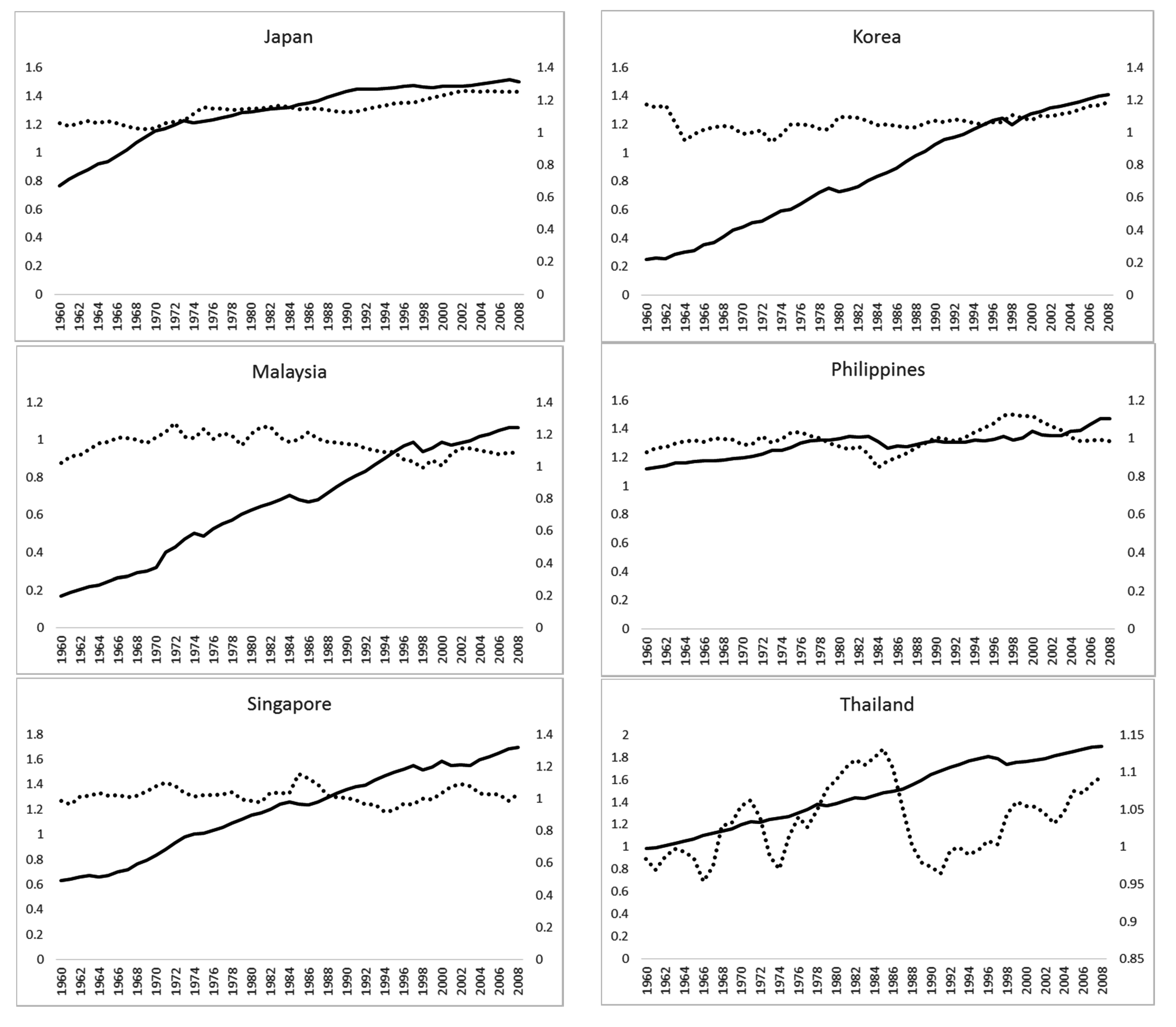
Figure 1 provides two-scale time-series plots of logarithms of government-share (right scale) and real GDP per capita (left-scale), depicting the temporal evolution of the two variables in each of the six countries. It is reasonable to say that the increase in log GDP per capita is not accompanied by a discernible increase in log government share except in Japan. For example, while real GDP per capita shows steady growth in all countries during the period, government-share shows a perceptible increase, mainly in Japan, and the government-share plots are largely flat in most cases. As for the Philippines, while real GDP per capita has a modest growth rate, government-share seems stagnant. Therefore, the simple plots suggest lack of a discernible support for the hypothesis except for Japan and possibly for the Philippines.
As Ram (1998 [
20], pp. 149–150) has pointed out, the Wagnerian hypothesis is primarily a statement about the long-run positive covariation between two increasing variables. However, almost all research has formulated the hypothesis in a regression framework and has tried to draw inferences about the hypothesis from a variety of estimation procedures. We proceed with that approach to formally test the validity of the hypothesis.
Figure 1.
Evolution of logarithms of per capita real GDP (solid, leftscale) and of government share (dots, right scale): 1960–2008.
Figure 1.
Evolution of logarithms of per capita real GDP (solid, leftscale) and of government share (dots, right scale): 1960–2008.
There are at least six alternative specifications of Wagner’s law (Mohammadi
et al., 2008 [
21]; Payne
et al., 2006 [
22]). Peacock and Wiseman (1979) [
23] model the log of real government expenditures as a function of the log of real output. Support for the hypothesis requires that the elasticity of government expenditures with respect to output exceed unity. Mann (1980) [
24] models the share of government expenditures in total output as a function of real output per capita. The validity of Wagner’s hypothesis requires that the elasticity of government share with respect to output exceed zero. Musgrave (1969) [
25] models the share of real government expenditures to output as a function of real per capita output. The validity of the hypothesis requires the elasticity of government expenditures with respect to real output per capita exceed zero. Gupta (1967) [
26] models real per capita government expenditures as a function of real per capita output. Support for the hypothesis requires that the elasticity of per capita real government expenditures with respect to real per capita output exceed unity. Goffman (1968) [
27] models the real government expenditures as a function of real per capita output. Support for the hypothesis requires that the elasticity of real government expenditures with respect to per capita output exceed unity. Finally, Pryor (1968) [
28] models real government consumption expenditures as a function of real output. Support for the hypothesis requires that the elasticity of government consumption with respect to income exceed unity.
We utilize the specification proposed by Mann (1980) [
24] due to its parsimonious nature and limited data requirements, and examine the long-run relation between log of government share (LGS) and log of real GDP per capita (LRYPC) using tests of cointegration. More specifically, let LGS and LRYPC be nonstationary in levels but stationary in first-differences. As Engle and Granger (1987) [
29] have pointed out, a linear combination of LGS and LRYPC, if stationary, implies the existence of a long-run relationship between them. The stationary linear combination is referred to as the cointegrating equation, and may be interpreted as the long-run equilibrium relationship.
Table 4 reports test statistics for cointegration vectors using the maximum-likelihood procedure proposed by Johansen (1996) [
30]. Both trace and maximum eigenvalue statistics reject the null hypothesis of no-cointegration for Japan and Korea but fail to reject the null for the remaining four countries. Thus, maximum-likelihood tests of cointegration provide a rather weak support in favor of the Wagner’s hypothesis.
Table 4.
Maximum likelihood tests of cointegration.
Table 4.
Maximum likelihood tests of cointegration.
| | Japan | Korea | Malaysia | Philippines | Singapore | Thailand | 5% c.v. |
|---|
| Trace test |
| r = 0 | 22.054 * | 23.367 * | 12.707 | 5.147 | 12.055 | 10.223 | 15.497 |
| r ≤ 1 | 4.809 | 1.596 | 1.862 | 0.335 | 1.645 | 1.505 | 3.841 |
| Max-Eigen test |
| r = 0 | 17.246 * | 21.771 * | 10.844 | 4.812 | 10.410 | 8.718 | 14.255 |
| r ≤ 1 | 4.809 | 1.596 | 1.862 | 0.335 | 1.645 | 1.505 | 3.641 |
A potential shortcoming of the maximum likelihood procedure is that its test outcomes may be affected by the possible presence of structural breaks. To address this issue, we implement the residual-based test proposed by Gregory and Hansen (1996) [
31] in the presence of on endogenously-identified structural break. The results, reported in
Table 5, support the hypothesis of no-cointegration in every case.
2
Table 5.
Gregory-Hansen’s tests of cointegration with one structural break.
Table 5.
Gregory-Hansen’s tests of cointegration with one structural break.
| Country | Minimum t-Statistics: Model (LGS, LRYPC) |
|---|
| Japan | −3.448 (1995) |
| Korea | −3.870 (1998) |
| Malaysia | −4.074 (1988) |
| Philippines | −4.455 (2001) |
| Singapore | −2.862 (1997) |
| Thailand | −2.980 (2000) |
The main conclusion emerging from
Table 4 and
Table 5 is that while, as is often observed in such tests, there is considerable diversity in the test outcomes, one might infer some evidence of cointegration for Japan and Korea, but not in other cases.
It is possible that lack of cointegration might be due to the fact that while the tests are based on symmetric adjustments to deviations from the long-run equilibrium, the adjustments are actually asymmetric. Therefore,
Table 6 reports the Momentum Threshold Autoregressive (MTAR) test proposed by Enders and Siklos (2001) [
13] to judge whether the variables are cointegrated and whether the adjustments are asymmetric. It is evident from the table that the null hypothesis of no-cointegration cannot be rejected for each of the six countries. This is reflected in the values of
statistics which are well below the 5% critical value of 11.47. These findings are consistent with results reported in Table 5.
3
Table 6.
Tests of cointegration and asymmetric adjustments (MTAR model).
Table 6.
Tests of cointegration and asymmetric adjustments (MTAR model).
| Country | | | | | | |
|---|
| Japan | −037 | −0.491 (0.199) | −0.252 * (0.110) | 4.825 | 1.135 | 36.541 * |
| Korea | −0.052 | −0.598 (0.407) | −0.402 * (0.125) | 5.846 | 0.475 | 20.256 |
| Malaysia | −0.024 | −0.351 (0.215) | −0.225 (0.121) | 2.896 | 0.521 | 9.760 |
| Philippines | 0.050 | −0.275 (0.184) | −0.142 (0.075) | 2.732 | 0.681 | 9.751 |
| Singapore | −0.018 | −0.206 (0.225) | −0.399 * (0.127) | 5.209 | −0.778 | 11.992 |
| Thailand | −0.037 | −0.020 (0.303) | −0.185 (0.079) | 2.686 | −0.535 | 17.280 |
The tests in
Table 4,
Table 5 and
Table 6 are conducted for each country separately. It is possible to conduct panel cointegration tests of the kind proposed by Pedroni (2004) [
14] by pooling the data. An attractive characteristic of Pedroni’s tests is that they permit heterogeneity in intercept and “slopes” across the countries and thus combine the merit of using individual-country data with the advantage offered by much larger sample size. Pedroni (1999 [
33], 2004 [
14]) has proposed seven test statistics for the null hypothesis of no-cointegration in panel data. The first four tests are referred to as the within-dimension tests or panel statistics tests, and assume a homogenous autoregressive coefficient for all cross sections under the alternative hypothesis. The remaining three tests are referred to as between-dimension or group statistics, and assume heterogeneous autoregressive coefficients for all cross sections under the alternative hypothesis. Thus, the alternative hypothesis in both within- and between-dimension tests seven tests is the rejection of the null hypothesis of no-cointegration across all cross sections.
Table 7 reports the results of seven test statistics for the null of no-cointegration associated with Pedroni’s procedure. The evidence is mixed. Looking at within-dimension tests, the panel PP- and panel ADF-statistics reject the null hypothesis of no-cointegration while panel v- and panel rho-statistics fail to do so. Similarly, the group ADF-statistic from the between dimension tests reject the null hypothesis of no-cointegration while the remaining two tests (group rho- and group PP-statistics) fail to do so. Thus, there are some indications of cointegration between government share and real GDP per capita in panel data.
Table 7.
Pedroni’s panel cointegration test statistics.
Table 7.
Pedroni’s panel cointegration test statistics.
| Test Statistics | Model (LGS, LRYPC) |
|---|
| I. Within Dimension | |
| Panel v-statistic | 0.703 (0.241) |
| Panel rho-statistic | −0.757 (0.225) |
| Panel PP-statistic | −1.929 (0.027) * |
| Panel ADF-statistic | −2.697 (0.003) * |
| II. Between Dimension | |
| Group rho-statistic | 0.564 (0.714) |
| Group PP-statistic | −0.961 (0.168) |
| Group ADF-statistic | −2.183 (0.015) * |
To the extent cointegration between government share and real income may be considered necessary or relevant for inferring support for the hypothesis,
Table 4,
Table 5,
Table 6 and
Table 7 seem to convey a highly variable scenario that makes it difficult to draw a sharp conclusion. Nevertheless, one could say that the broad picture emerging from these tests is largely consistent with the view yielded by
Figure 1 of limited support for the hypothesis relative to Japan and possibly Korea.
3. Concluding Observations
Noting the paucity of research relative to high-growth East Asia in the extensive literature on Wagner’s hypothesis, we study the empirical status of the hypothesis from annual data for six countries covering the 49-year period 1960–2008. Our methodology ranges from the old-fashioned consideration of graphs to sophisticated time-series and panel cointegration tests. Seven points summarize the outcome of the exercise. First, a variety of tests of unit roots suggest that both government shares and real per capita GDP are non-stationary in levels but stationary in first-differences; Second, the temporal evolution of government-share and real GDP per capita indicate support for the hypothesis in Japan, but lack of support in the other countries; Third, Johansen-type maximum-likelihood tests largely support cointegration for Japan and Korea, although there is some variability across the two test formats; Fourth, however, Gregory-Hansen tests that are based on one endogenously-identified structural break do not support cointegration for any of the countries; Fifth, MTAR models of Enders and Siklos indicate lack of cointegration; Sixth, Pedroni’s tests of panel cointegration, which permit cross-country heterogeneity in the constant term and the “slope” coefficients, provide mixed results; Seventh, our overall conclusion thus has two parts. Substantively, despite high growth rates in almost all the six countries, Wagner’s hypothesis is not supported for Malaysia, the Philippines, Singapore and Thailand. Methodologically, while the pattern is reflected fairly well in the plots, the widely-used cointegration methodology yields a diverse scenario.
We should add that although the substantive conclusion stated above seems reasonable, some shortcomings of our work may be noted. For example, despite its extensive usage, our measure of government-share is an incomplete proxy for the size of the public sector. Also, our exploration is somewhat conventional and abstracts from the refinements suggested by Biehl (1998) [
15]. Perhaps more important, this is primarily an exploration of the empirical evidence on Wagner’s hypothesis in these countries, and an explanation for the observed lack of cointegration in most cases is beyond the scope of the work. However, we note a few conjectures about the observed pattern: (1) our government-size variable includes purchase of goods and services by the government, but does not include transfer payments which often increase with economic development. Our measures may thus tend to dilute the evidence in favor of the hypothesis; (2) the measure does not include outlays by public-sector enterprises which may also affect the evidence; (3) it has been suggested that evidence on the hypothesis may depend on the level of development of a country, and that might explain support for the hypothesis in Japan and, to some extent, in Korea; (4) operation of the hypothesis may partly depend on the political orientation of the government. While conservative regimes may be associated with weaker evidence in favor of the hypothesis, public sector with a “liberal” orientation might strengthen the evidence favoring the hypothesis. It is, however, difficult to judge the overall orientation of the public sector over a long period. Lastly, while there may be some expectation that the hypothesis should hold when a long period is considered, our conclusions are broadly consistent with a large segment of the literature that indicates lack of evidence in favor of the hypothesis.


