Impact of Fiscal Policy on Consumption and Labor Supply under a Time-Varying Structural VAR Model

Faculty of Economics and Finance, Effat University, Jeddah 22332, Saudi Arabia
Economies 2019, 7(2), 57; https://0-doi-org.brum.beds.ac.uk/10.3390/economies7020057
Submission received: 5 May 2019
/
Revised: 3 June 2019
/
Accepted: 13 June 2019
/
Published: 17 June 2019
(This article belongs to the Special Issue Computational Macroeconomics)
Abstract
:This paper investigates the impact of fiscal policy on private consumption and labor supply in the UK economy using time-varying parameter vector autoregression (TVP-VAR) with stochastic volatility for the period Q2 1987 to Q2 2017. It considers fiscal variables such as government expenditure and net tax revenue and evaluates their impact on private consumption and average hours worked per week. Three sample periods were selected and two approaches were used to identify impulse responses, first taking the average of stochastic volatility over the sample period, and then allowing for sign restrictions based on contemporaneous relationships among the selected variables. The study found a negative wealth effect of public spending on private consumption and a positive effect on hours worked, as people tend to work more hours to maintain the same standard of living. Similarly, a tax shock generates negative effects on consumption but the impact on worked hours remains unclear over a three-year time horizon. These findings are almost consistent across sample periods and alternative specifications of impulse responses. This is one of only a few studies to determine the linkages between fiscal policy and the labor market using a macroeconomic framework.
JEL Classification:
C55; E21; E24; F621. Introduction
The Great Recession of 2008 revived interest in the role of fiscal policy, and there has been an increase of studies in the literature evaluating the stabilizing role of government spending and taxes, especially in the context of ineffective monetary policy due to the zero lower bound on nominal interest rates. In response to the onset of the recession, many countries adopted fiscal stimulus programs to boost aggregate demand. In the United Kingdom, the government introduced various tax cuts and increased government spending. However, the government was constrained in its pursuit of fiscal stimulus because of the huge bank bailouts made necessary by the banking crisis. These led to an immense burden on public finance and debt rose to 80% of gross domestic product (GDP). This study aims to investigate the impact of these fiscal policies on consumption and labor supply in the UK economy during this period.
Historically, the mechanism of transmission of fiscal policy is explained by two strands of theory. On the one hand, there is Keynesian tradition, which assumes sticky prices in the short run. Consequently, an expansionary fiscal policy leads to higher aggregate demand, boosting income and employment, and thus, through multiplier effects, higher consumption. This type of transmission mechanism, where output is determined by demand, is known as the aggregate demand effect of fiscal policy (e.g., Taylor 2000; Fatas and Mihov 2001; Blanchard and Perotti 2002; Perotti 2005 and Galí et al. 2007).
The second strand follows neoclassical synthesis, which assumes fully flexible prices. Here, fiscal policy affects the economy through a negative wealth effect. The tax financing of increased government expenditure transmits a negative wealth shock to households by reducing their permanent income, and consequently they start consuming less and working more hours. In a neoclassical model with an unchanged labor demand curve, the labor supply curve shifts out, leading to a lower real wage rate (Baxter and King 1993). Therefore, the outcomes of the neoclassical general equilibrium model are opposite to the Keynesian aggregate demand model in terms of real wage rate and private consumption. Alternatively, the responses of private consumption and real wage rate to a government spending shock can potentially be used to distinguish between different models.
The research in this paper contributes to the literature on fiscal policy and the labor market in the UK with a time-varying parameter vector autoregression (TVP-VAR) model with stochastic volatility, which allows us to capture possible changes in the underlying structure of the economy. Initially, at the time of the 2008 recession, the UK government followed a strong counter-cyclical fiscal expansion. This was reversed in 2010, which led to a debate on austerity measures and their impact on the economy. More recently, there has been a resurgence of this policy debate in the context of Brexit and its consequences to the labor market. Therefore, this research contributes to the literature to determine the linkages between fiscal policy, aggregate demand, and the labor market in the context of the current policy debate.
To date, most of the empirical research on fiscal policy has focused on the US economy (Auerbach and Gorodnichenko 2012; Bachmann and Sims 2012; Ramey and Zubairy 2014). In the UK, the debate has concentrated on the issue of austerity versus fiscal stimulus. Austerity is favored to restore the confidence of the financial markets through sustainable public debt (Rogoff 2013), and it could possibly crowd in private consumption and investment (Trichet 2010). However, austerity is criticized based on large fiscal multipliers in a recession due to the lower capacity utilization rate and constrained monetary policy (Krugman 2015), and in this context austerity measures may induce negative effects on the economy. DeLong and Summers (2012) suggest that austerity in a depressed economy can erode the long-term fiscal balance. Moreover, earlier studies on UK fiscal policy mainly concentrated on the estimation of fiscal multipliers for output and unemployment. These studies include (Cimadomo and Benassy-Quere 2012; Baum et al. 2012; Crafts and Mills 2013; Rafiq 2014; and Glocker et al. 2017).
This research extends the literature by employing a time-varying parameter structural VAR specification, which allows both a temporary and permanent shift in the parameters. Stochastic volatility is an important attribute of the TVP-VAR model. The idea of stochastic volatility was first presented by Black (1976), followed by various developments in financial econometrics such as Ghysels et al. (1996) and Shephard (2005). Stochastic volatility has been commonly used in recent years for the empirical analysis of macroeconomic dynamic relationships (e.g., Uhlig 1997; Cogley and Sargent 2005; Primiceri 2005; and Nakajima 2011). If a data-generating process of economic variables has shocks of stochastic volatility and drifting coefficients, applying time-varying coefficients with constant volatility will lead to biased estimates, because possible variation of the volatility in disturbances is ignored.
This research employs the Markov chain Monte Carlo (MCMC) method to generate the posterior estimates for our TVP-VAR model, the estimates of the convergence diagnostics (CD) of Geweke (1992), 95% credibility intervals, and the inefficiency factors to reveal the efficient posterior distribution of the model. The posterior estimates of stochastic volatility of a structural shock also indicate the presence of volatility for all variables in the model, which justifies the use of the time-varying parameter structural VAR model to observe the linkages between fiscal policy, aggregate demand, and the labor market. We specify the impulse responses under two alternative schemes: first, we consider the average of stochastic volatility over the sample, and the second approach is based on sign restrictions. Both approaches show a negative wealth effect of government spending, which leads to crowding out of household consumption, and with a time lag, average weekly hours worked starts to rise, which is logical, as people start working more to maintain a similar standard of living.
2. Literature Review
The role of fiscal policy in affecting macroeconomic dynamics is an old debate in both the theoretical and empirical literature. There is no clear consensus on the transmission channels of fiscal policy, the size of the multiplier in the short term, and the impact on long-term growth. While there is some agreement on the impact of government expenditure on output, there remains disagreement on the effects of expenditure shocks on consumption and real wage rates. According to the Keynesian view, a spending shock leads to higher consumption and wages (e.g., Rotemberg and Woodford 1992; Blanchard and Perotti 2002; Galí et al. 2007). While some authors have shown that private consumption decreases in response to a government spending shock (e.g., Baxter and King 1993; Ramey and Shapiro 1998; Hall 1986; Cogan et al. 2009; Farmer and Plotnikov 2012), others have shown that public spending and private consumption are either complements or substitutes (Aschauer 1985; Karras 1994; Ni 1995; Amano and Wirjanto 1998; Okubo 2003).
Apart from these theoretical differences over the impact of fiscal shocks on consumption and wages, there is a large debate on the best way to identify fiscal shocks, which has led to methodological discrepancies. Models based on structural vector autoregression (SVAR), such as that of Blanchard and Perotti (2002), tend to show an increase in consumption in response to government spending shocks. On the other hand, the narrative approach developed by Ramey and Shapiro (1998) identifies large decreases in private consumption due to public spending shocks. This narrative approach isolates three events of large military expenditure in the US (known as Ramey–Shapiro episodes) and identifies fiscal shocks to an event-based dummy variable. Their research indicates that a government spending shock slightly decreases nondurable and service consumption, while this effect is mostly statistically insignificant. Following Ramey and Shapiro’s approach, Edelberg et al. (1999) and Burnside et al. (1998) also found a weak and statistically insignificant response of private consumption to the onset of a Ramey–Shapiro episode.
The empirical literature, which mostly examines the impact of public spending on private consumption, employs structural VAR models with different sets of identifying restrictions. A majority of these studies evaluate the relationships among error terms and variables in the structural form (Corsetti et al. 2009), impose structural restrictions on impulse responses (Enders et al. 2008), or incorporate external institutional information for an exhaustive analysis of lower frequency macro data and lags in fiscal decisions (Perotti 2005). Most of these studies show a positive correlation between public spending and private consumption (e.g., Blanchard and Perotti 2002; Galí et al. 2007).
Differentiating public spending as productive or nonproductive, Smets and Wouters (2007) developed and estimated a new Keynesian model. Their model considers only nonproductive government expenditure and assumes that any increase in debt to finance additional government expenditure is paid off through future taxes. Their results show crowding out for both private consumption and investment and spending shocks generating a small positive effect on GDP. Galí et al. (2007) include “rule-of-thumb” consumers and price rigidities in their model to examine the impact of public spending on private consumption. According to their model, non-Ricardian households cannot react to higher future taxes, as increased government spending leads to higher aggregate demand and sticky prices lead to higher real wages and consequently increased consumption. Linnemann and Schabert (2003) also reveal that sticky prices are not enough to generate a crowding-in effect of public spending shock in private consumption. Similarly, Ravn et al. (2006) indicate that deep habits with price rigidities can generate a positive reaction of private consumption to public spending. Studies such as those by Linnemann and Schabert (2006), Ambler and Paquet (1996), and Baxter and King (1993) suggest that productive public spending together with price rigidities can lead to a crowding-in effect of public spending on private consumption.
Linnemann (2006) used the link between marginal utility of consumption and labor hours along with the assumption that lump-sum taxes are residually determined through government budget constraint (ignoring distortionary taxes, debt, and any fiscal rules). He found that public spending can generate positive effects on private consumption. In contrast, Leeper et al. (2010) emphasized the role of fiscal rules for the US economy. They used productive government spending and examined the effects of delays on the implementation of preannounced public spending. Their research revealed the significance of debt financing and its implications and suggested that lump-sum taxes/transfers have no significant effect on private consumption. This is consistent with the empirical literature, which shows that responses of consumption to a public spending shock mainly depend on the way increased government expenditure is financed (e.g., Mountford and Uhlig 2009). To evaluate the spillover effects on the economy, Forni et al. (2009) considered different types of government spending with both Ricardian and non-Ricardian agents, but their research did not find any significant crowding-in effect of public spending on private consumption. Similarly, Coenen et al. (2012) suggested that we can observe a crowding-in effect on private consumption when the model is based on two assumptions: there is complementarity between private consumption and public spending, and government consumption is included in the utility function in an inseparable manner. This is consistent with models estimated by Kormilitsina and Zubairy (2016), who were not able to find a crowding-in effect of public spending on private consumption.
The literature examining the impact of fiscal policy on the labor market includes both empirical and theoretical analysis. Empirical studies have concentrated on the transmission of fiscal policy in the labor market through unemployment and output multipliers. Mostly these studies are based on structural vector autoregression models, which examine the responses of macroeconomic and labor market variables to shocks in public spending. Most of these studies determined a system of equations in a dynamic stochastic general equilibrium framework. For example, Yuan and Li (2000) examined the responses of employment and hours of work per employee to a shock in government expenditure for US data. They first estimated a structural VAR model to evaluate the responses of the output, employment, and hours per worker, and then developed a real business cycle (RBC) model with labor market frictions to observe similar responses to those of the structural VAR model. Monacelli et al. (2010) estimated structural VAR models for the US and calculated both the unemployment and output multipliers of government spending. Their results showed that an increase in public spending by 1% of GDP would generate output and unemployment multipliers of about 1.2% and 0.6 percentage points, respectively. Their RBC model with labor market frictions produced a similar output multiplier (with some special parameterization), but they were unable to reproduce a similar output multiplier.
Theoretically, increased government expenditure stimulates output and employment in the economy, as revealed by Yuan and Li (2000) and Monacelli et al. (2010). Mayer et al. (2010) developed a dynamic stochastic general equilibrium (DSGE) model with labor market frictions and liquidity-constrained consumers. Their research found that a positive shock in government expenditure would reduce aggregate unemployment with fewer liquidity-constrained consumers.
In general, the macroeconomic dynamic structure associated with uncertainty and volatility, therefore the empirical literature on VAR models with time-varying parameters and stochastic volatility, has grown in recent years. Researchers have mostly employed the TVP-VAR model to examine macroeconomic dynamic structures such as the relationships between inflation and employment (Cogley and Sargent 2001) and between output and the exchange rate (Mumtaz and Sunder-Plassmann 2010), and the impact of monetary policy (Primiceri 2005; Cogley and Sargent 2005; Canova and Gambetti 2009; Koop et al. 2009). However, Benati (2008) specified a TVP-VAR model with sign restrictions on the impulse response to examine the “great moderation” and inflation dynamics of the UK economy, whereas Kapetanios et al. (2012) employed a VAR model with time-varying parameters to examine the macroeconomic impact of quantitative easing on the UK economy. For the Euro zone, Baumeister et al. (2008) evaluated the impact of excess liquidity shocks on selected macroeconomic variables using a TVP-VAR model. Nakajima (2011) estimated a TVP-VAR model using Japanese macroeconomic time series.
Primiceri (2005) characterized VAR models with time-varying parameters as allowing for “drifting coefficients [that] are meant to capture possible nonlinearities or time variation in the lag structure of the model.” He further states that “multivariate stochastic volatility is meant to capture possible heteroscedasticity of the shocks and nonlinearities in the simultaneous relations among the variables of the model.” According to Kapetanios et al. (2012), the TVP-VAR model is more flexible than other time-varying VAR models, including the Markov-switching VAR (MS-VAR). They argued that the TVP-VAR model is appropriate during crises when economic agents are not clear about the impact of shocks on the structure of the economy.
This research aims to investigate the impact of fiscal policy on consumption and labor supply through a time-varying structural VAR model with stochastic volatility, as many recent empirical studies have identified the structural breaks in macroeconomic variables (Cogley and Sargent 2005; Primiceri 2005). This approach is advantageous for several reasons: First, it is flexible and capable of capturing both sudden and gradual changes in the underlying economic structure as well as the nonlinearity that may occur. Second, models with time-varying parameters and stochastic volatility are often found to forecast better than their constant coefficient counterparts (see, e.g., Clark 2011; D’Agostino et al. 2013; Clark and Ravazzolo 2015). Third, the TVP-VAR model allows the shocks to change over time, allowing volatility in errors, as many policy outcomes depend on this time variation. Finally, a TVP-VAR model is required to isolate the fiscal policy effects at different time points to indicate the time variation in coefficients, especially for the three selected sample periods.
3. Methodology
To evaluate the impact of fiscal policy on private consumption and labor supply, this study employs a time-varying parameter vector autoregression (TVP-VAR) model with stochastic volatility. This model is capable of capturing the time-varying nature of the underlying structure in the economy in a flexible and robust manner (Nakajima 2011). In a VAR model, the parameters follow a random walk process, indicating both temporary and permanent changes in the system. The main characteristic of the TVP–VAR model is the addition of stochastic volatility.
A time-varying model with constant volatility may give biased results when some economic variables have drifting coefficients and stochastic volatility. A time-varying VAR model with stochastic volatility avoids such issues and allows for simultaneous relationships among variables of the model and heteroscedasticity of the innovations (Primiceri 2005). However, intractable likelihood functions often make estimation difficult in case of stochastic volatility; therefore, the Markov chain Monte Carlo (MCMC) method can be used to estimate the model in the context of Bayesian inferences.
We identify the time-varying VAR model as follows:
where Zt is an n × 1 vector of observed endogenous variables, Ct is an n × 1 vector of time-varying coefficients that multiply constant terms, B(i,t), i = 1, …, k represents n × n matrices of time-varying coefficients, and μt represents heteroscedastic unobservable shocks with n × n time-varying variance covariance matrix Ωt. To specify the simultaneous relationships of the structural shocks, this model assumes recursive identification through the decomposition of , where is a lower triangular matrix with diagonal element equal to 1 and is allowed to vary over time, which implies that an innovation in the ith variable has a time-invariant effect on the jth variable (Nakajima 2011). This recursive structure follows a causal ordering of government expenditures, government revenues, personal consumption expenditures and weekly hours worked. An increase in government expenditures may leads to large tax hikes which in turn reduce personal consumption expenditures. In case, If people want to maintain same standard of living then they may work for more hours. Furthermore, , is defined as the stacked row vector of , is the stacked row vector of the free lower-triangular elements of , and where . In addition, the model assumes the time-varying parameters follow a random walk process.
For with , where and are diagonal matrices, , , and .
To estimate the time-varying model, this study employs Bayesian inference through the MCMC method, which helps to examine the joint posterior distribution of the parameters under certain prior probability densities.
Following Nakajima (2011), we assume the priors such as , where and G represent the inverse Wishart and gamma distributions and and are the diagonal elements in and , respectively. Furthermore, we assume flat priors for our model such as and .
We examined the UK economy for the sample period 1987 Q2 to 2017 Q2, considering fiscal variables such as government expenditure, tax revenue, and labor market variables including average hours worked per week. The data for these variables were extracted from the Office for National Statistics database (Table 1). All variables were transformed into growth rates to ensure stationarity for the selected data series. The estimation is based on two lags suggested by lag selection criterion such as the Akaike information criterion, Hannan–Quinn criterion, and Schwarz information criterion estimated through constant parameter VAR.
4. Results and Discussion
To evaluate the impact of fiscal policy on selected variables, we first identified a four-variable TVP-VAR model considering private consumption, weekly hours worked, government expenditure, and net tax revenues. This study considers fewer variables and this is a concern as it may leads to omitted variable bias; therefore we suggest alternative specifications for future research.
To obtain the posterior estimates for the TVP-VAR model, we drew the 10,000 samples after the initial 1000 were discarded during the burn-in period. Table 2 presents the estimates of posterior means with standard deviations, 95% credibility intervals, the convergence diagnostics (CD) of Geweke (1992), and the inefficiency factors computed through the MCMC method. The 95% credibility intervals include the estimates for posterior means and are Bayesian equivalents of the confidence intervals. Table 2 shows that all posterior means fall inside the credible intervals, indicating that the MCMC algorithm produces efficient posterior distribution.
Furthermore, CD is estimated through a test for equality of the means of the first and last parts of a Markov chain, as proposed by Geweke (1992). The test statistic is a standard Z-score: the difference between two sample means divided by the estimated standard error. These two means are equal and the test statistic has an asymptotically standard normal distribution if the samples are drawn from the stationary distribution of the chain. Table 2 reveals that our convergence diagnostics equals less than 1, therefore we cannot reject the null hypothesis that the Markov chain is in the stationary distribution. The last column in Table 2 indicates the inefficiency factor (IF) for the posterior estimates. The IF shows how well the chain mixes, and it is estimated as (), where is the kth autocorrelation of the chain. IF values below or around 20 are regarded as satisfactory. Table 2 shows that the IF values are significantly low for the time-varying coefficients (βs), therefore the results show that the MCMC algorithm efficiently produces posterior draws.
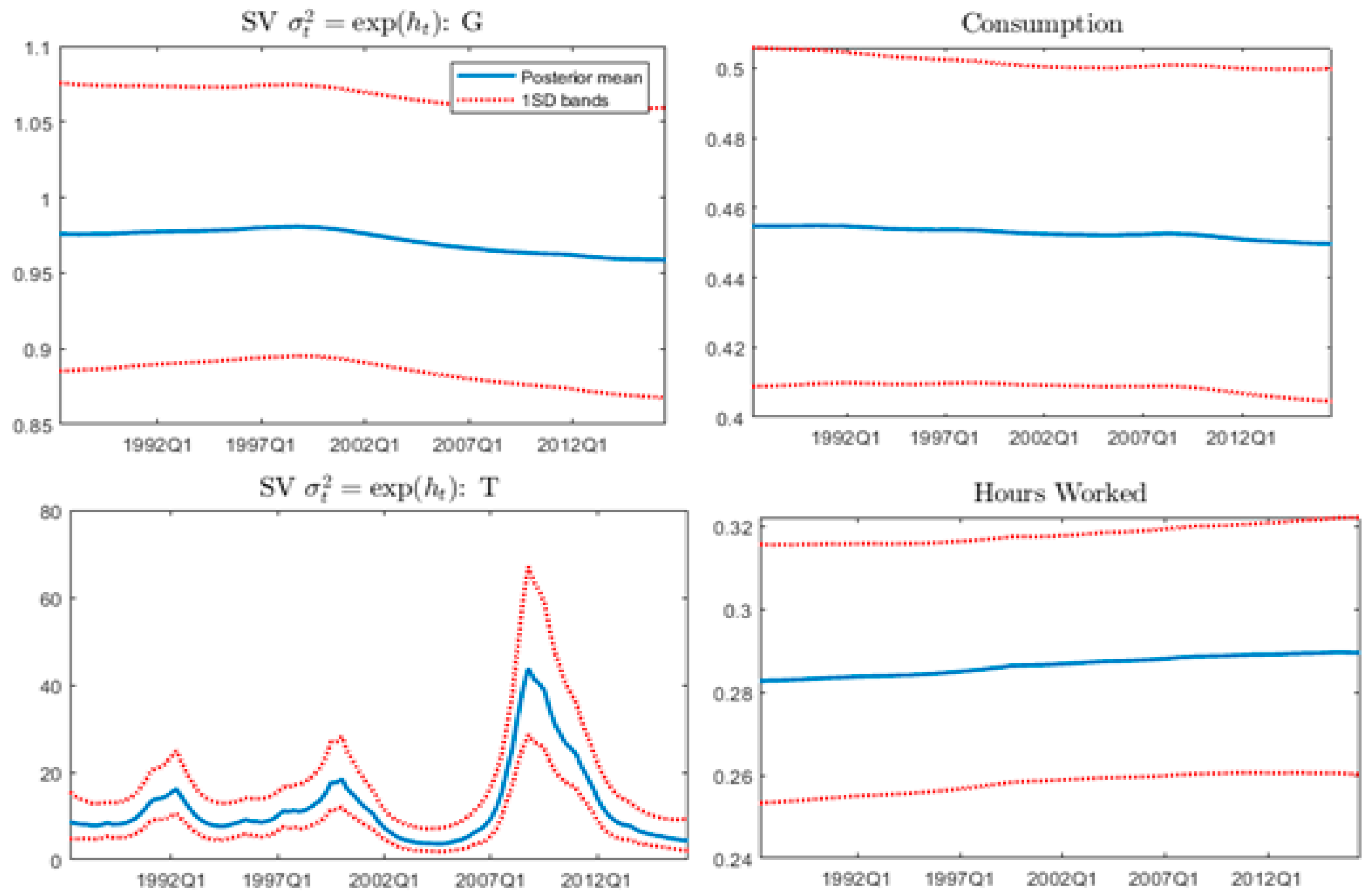
Figure 1 presents the posterior estimates of stochastic volatility of a structural shock for each variable used in the TVP-VAR for the period Q1 1987 to Q2 2017. The solid line indicates the posterior mean estimates and dotted lines show the 95% credible intervals. The estimates for the stochastic volatility shock identify two regimes: pre and post recession of 2008. The volatility estimates for the growth rates of government expenditure, private consumption, and hours worked are positive but relatively lower and smoother. However, volatility estimates are relatively higher for tax revenues and there is a spike during the financial crisis. Henceforth, these nonsteady and positive volatility estimates justify the use of the TVP-VAR model to capture the time-specific changes in the model.
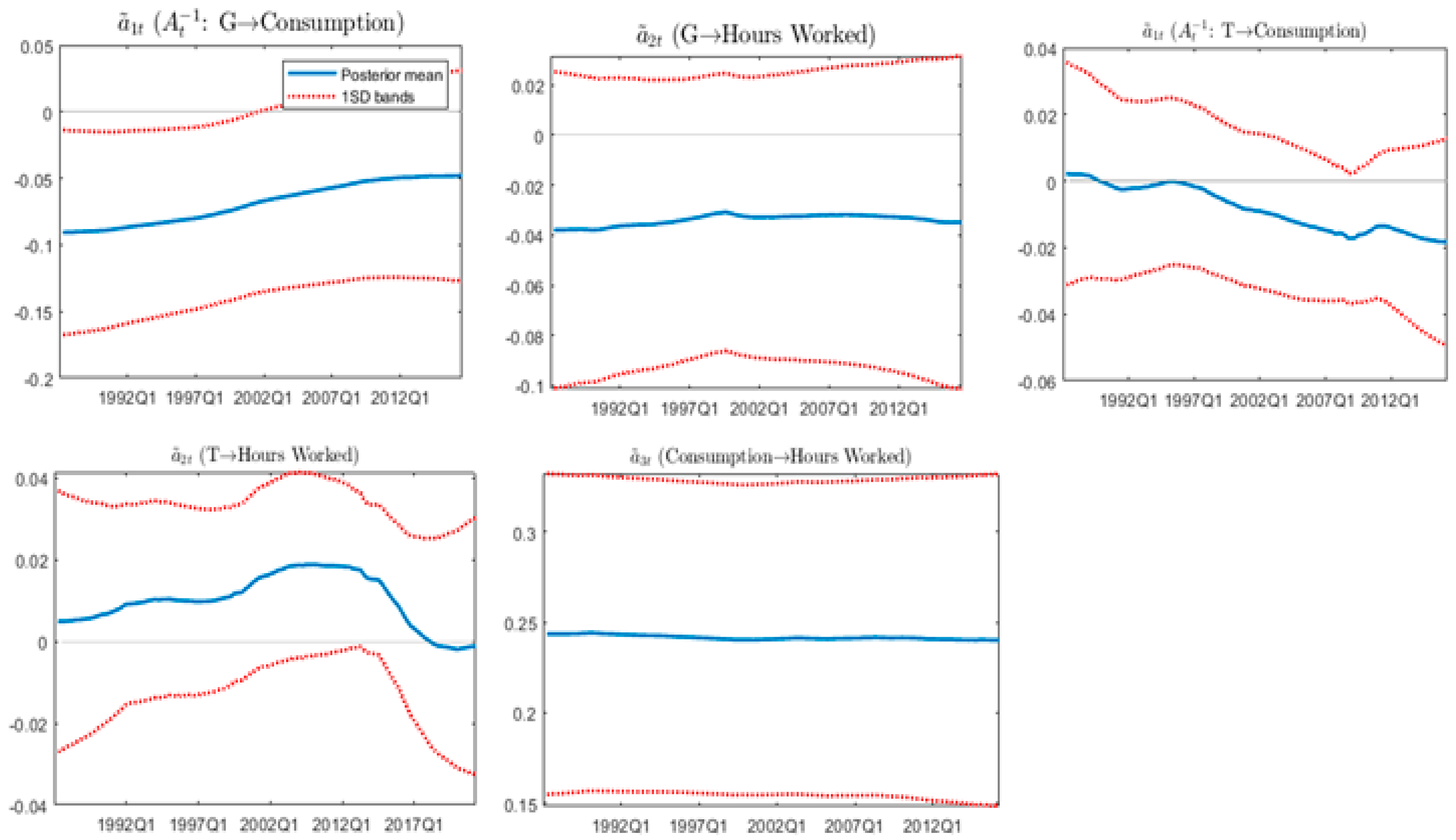
The time-varying simultaneous relationships among the variables are an important attribute of the TVP-VAR model. To estimate the simultaneous relationships, we specify a lower triangular matrix and the posterior estimates of the free elements in , plotted as in Figure 2, which depicts the size of the simultaneous effects of other variables to one unit of the structural shock.
The simultaneous relationship between the growth rates of government expenditure and private consumption remains negative and varies over the sample period, moving from −0.9 in 1987 to −0.05 in 2017. Figure 2 also reveals a negative relationship between the growth rates of government expenditure and average weekly hours worked; however, it remains constant over time. The simultaneous relationship between growth rates of taxes and private consumption remains negative from 1997 onward.
The parameters of a VAR system prompt the impulse response functions to capture the dynamics of the macroeconomic system. For a TVP-VAR model, we can compute responses at each point in time through time-varying parameters using restrictions on the parameter estimates of the model. Following Nakajima (2011), we compare responses over the time horizon by first setting the size of initial shock equivalent to the time series average of stochastic volatility over the sample period and then computing the impulse responses for the model. The estimated time-varying parameters are used from current data to future periods to compute the recursive innovation of the selected variable. In addition, we set these time-varying coefficients to be constant around the end of the sample period.
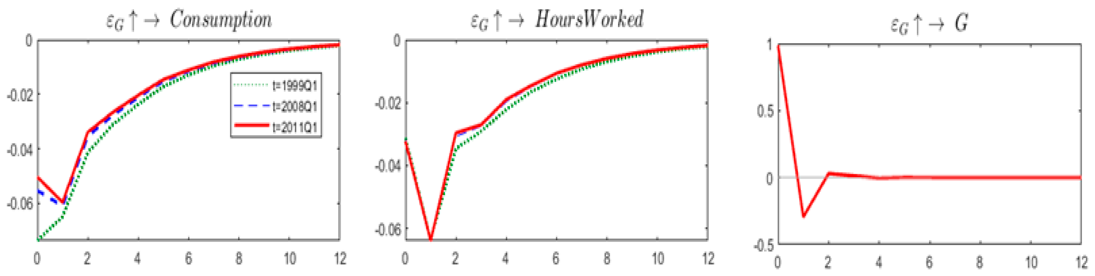
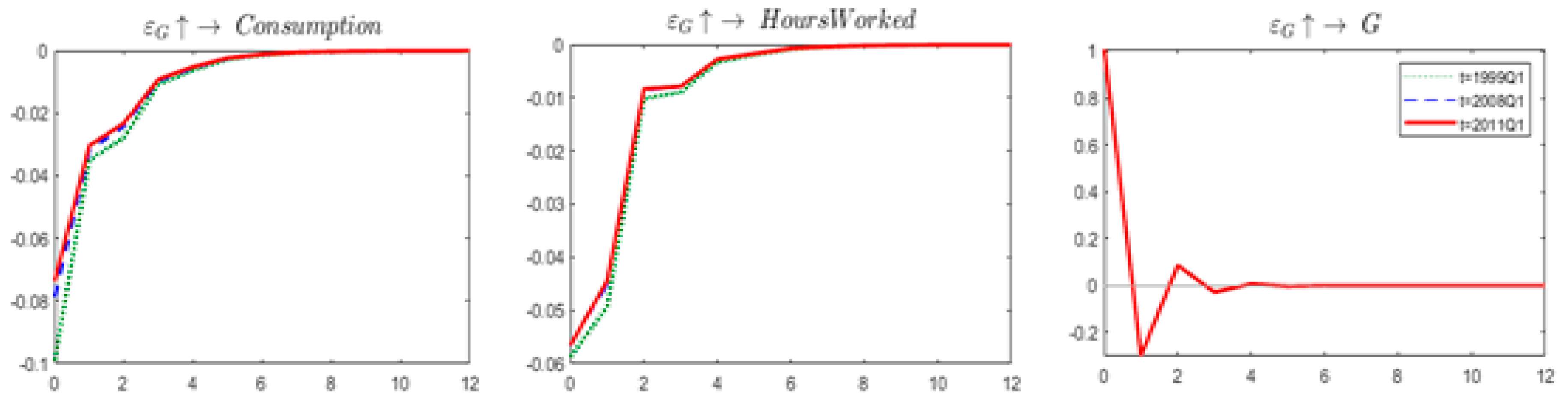
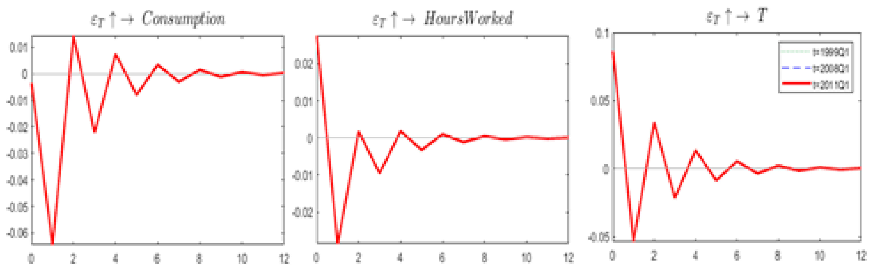
Since in a TVP-VAR model coefficients can vary over time, we can compute different sets of impulse responses at each point in the sample period. However, to specify our generalized impulse response functions, we select three time periods: Q1 1999, as shown by the structural break test; Q1 2008 as the period of the great recession; and Q1 2011 as the recovery period from the recession.
Figure 3 presents the impulse responses of government spending shock for the three selected sample periods. It shows that expenditure shock has a negative effect on consumption, although it is reduced in size (in absolute value) over the time horizon of three years. Moreover, the labor supply elasticity response to an expenditure shock is negative, and it becomes zero over the time horizon of three years. However, the expenditure shock on three different dates has effects of almost similar magnitude, which indicates less time variation in the estimated coefficients.
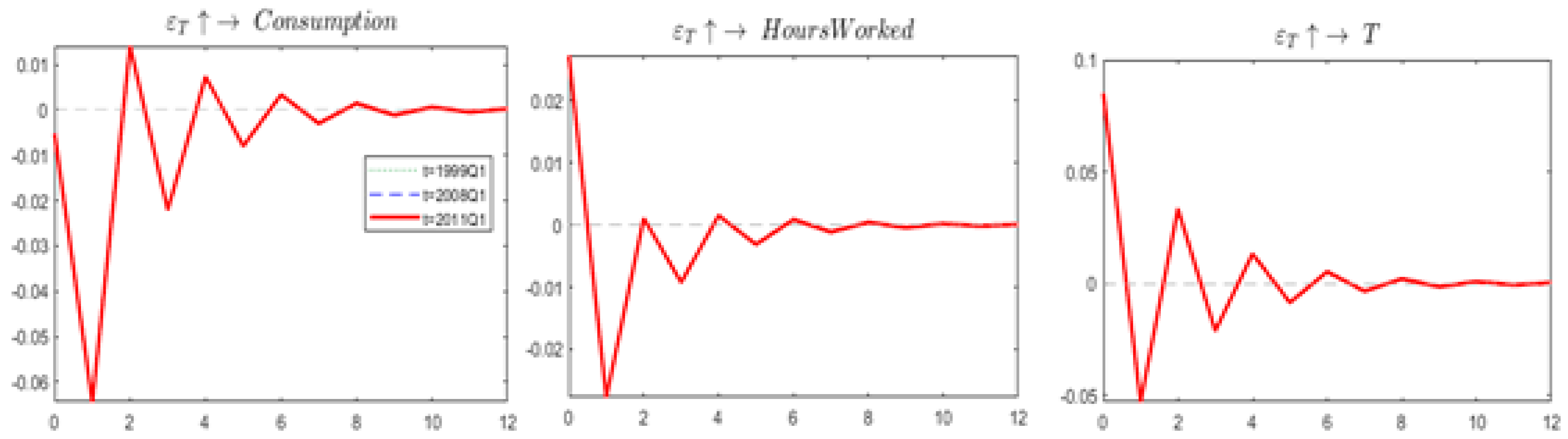
Figure 4 presents impulse responses of a tax shock on private consumption and hours worked. Initially, it shows a negative relationship between tax revenue change and private consumption; however, this relationship becomes slightly positive in the second quarter. In addition, the labor elasticity responses to a tax shock are smaller and differ across the sample periods. Initially, a tax shock has a positive effect on hours worked, but over time fluctuates between negative and zero values. Furthermore, both tax multiplier and labor elasticity values show no variation across the sample periods. Therefore, we conclude that a positive fiscal policy (both government expenditure and tax revenue) shock leads to lower consumption but its effect on worked hours is unclear. In case of a positive expenditure shock, worked hours remain negative whereas a positive tax shock first reduces the worked hours and then they increase in the next phase therefore impact of a tax shock on worked hours is unclear.
In addition, following Ellis et al. (2014), we identify the structural shocks through sign restrictions on the impulse responses of the variables to structural shocks. We impose these restrictions based on the simultaneous relationships observed in Figure 2. A positive shock in government expenditure leads to a higher tax burden for households, which in turns induces lower consumption in the economy. According to the neoclassical argument, a negative wealth effect motivates households to work more hours to maintain their standard of living, therefore this study uses a negative sign for private consumption and a positive sign for hours worked (Table 3).
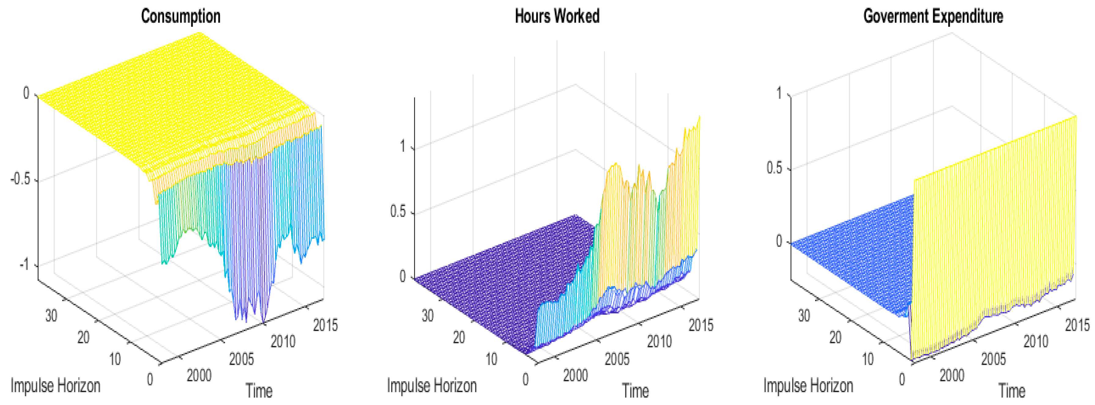
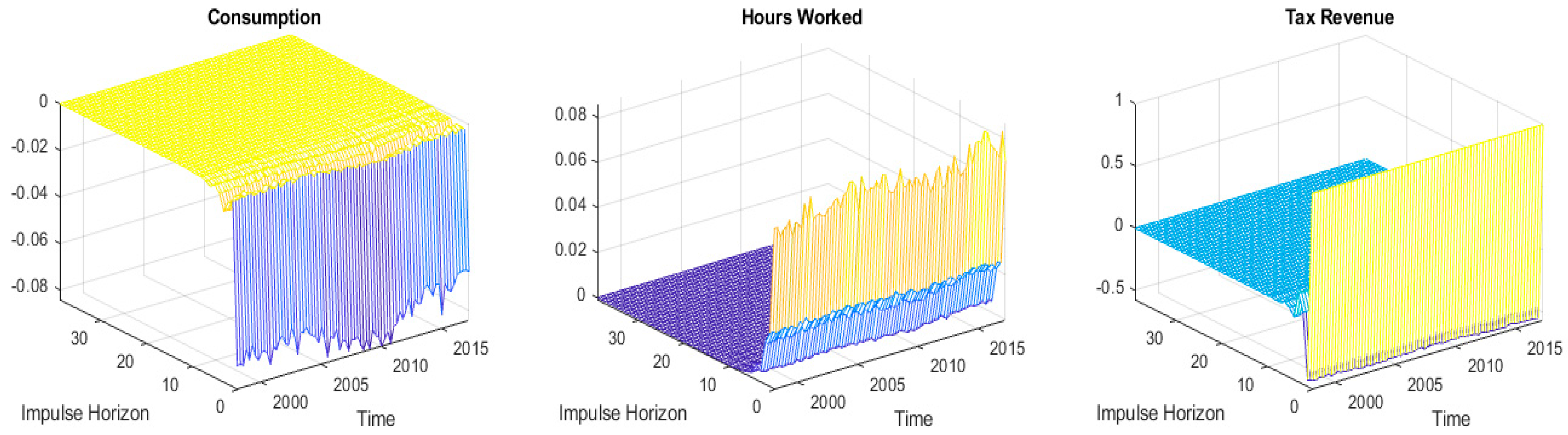
For time-varying impulse responses, we can draw a three-dimensional plot, as shown in Figure 5, which presents the reaction of private consumption and average weekly hours worked to shocks in government expenditure and taxes. We analyzed the contemporaneous relationships over time, different horizons, and magnitude. Figure 5 and Figure 6 present the median responses at each point in time. The x-axis shows the time period, the y-axis indicates the impulse response horizon, and the z-axis represents response values.
Figure 5 shows negative effects of a government expenditure shock on private consumption; a 1% increase in government expenditure decreases private consumption over time, which can be attributed to the negative wealth effect of public spending. In addition, an increase in public spending leads to more hours worked, and this positive elasticity of the labor supply can be attributed to the neoclassical argument that relates this outcome to tax financing of current public spending, as higher taxes lead to lower after-tax income, and to maintain their standard of living, people start working more hours. In addition, it can also be attributed to higher employment due to large public spending; however, crowding out of private consumption weakens this argument.
Figure 6 also depicts the neoclassical argument that a positive tax shock leads to more hours worked; the magnitude of this tax elasticity of the labor supply is small but positive. A positive tax shock also reduces private consumption, although the tax multiplier is smaller (Figure 6). In addition, Figure 3 and Figure 4 reveal that the spending elasticity of the labor supply is greater than the tax elasticity of the labor supply, which suggests a positive impact of fiscal policy on employment in the UK economy.
Therefore, our findings suggest that a positive spending shock has a negative wealth effect on private consumption under both types of impulse responses identified. These findings are consistent with Afonso (2008). A positive spending shock first has negative effects on hours worked and gradually this starts to reduce (absolute value). In addition, we find negative effects of a tax shock on private consumption and varying elasticity of the labor supply. Under both types of schemes, a positive tax shock leads to lower private consumption, whereas when we consider average stochastic volatility generating impulse responses at that time, it shows varying effects on the elasticity of the labor supply. As the negative wealth effect of public spending causes people to work more hours and tax financing emerges in the future, the moment it takes place, people are already working more hours. The impulse responses generated through the sign-restricted approach suggested by Ellis et al. (2014) indicates positive elasticity of the labor supply in response to a positive tax shock. We also confirmed these findings through alternative specification of sample periods and a set of priors (Appendix A and Appendix B).
5. Conclusions
This study employs a time-varying parameter VAR (TVP-VAR) model with stochastic volatility to examine the impact of fiscal policy on private consumption and labor supply. This model allows us to capture the uncertainty and drift of parameters at each time point in the sample, as most of the macroeconomic dynamic structures are characterized by volatility and fluctuations. This study employs total government expenditure and net tax revenue as fiscal policy variables and considers private consumption with average weekly hours worked to represent the labor supply variable for the sample period Q2 1987 to Q2 2017. This study finds a short-term “negative wealth” or “crowding out” effect of government expenditure on private consumption and a positive effect on hours worked. Similarly, a tax shock has negative effects on consumption, however the impact on worked hours remains unclear over the time horizon of three years. These results are consistent under two alternative specifications of impulse responses, including the average of stochastic volatility over the sample period as well as the sign restrictions based on contemporaneous relationships among the variables. In the United Kingdom, the role of fiscal policy has been a focus of considerable debate as to the choice between fiscal stimulus or austerity measures. This study provides important insights on the potential effects of fiscal measures on household final consumption and labor supply. However, our analysis is based on a broader macroeconomic structure and the labor market dynamics are mostly grounded in a micro framework, which could lead to further exploration in future work.
Funding
This research received no external funding.
Conflicts of Interest
The author declares no conflict of interest.
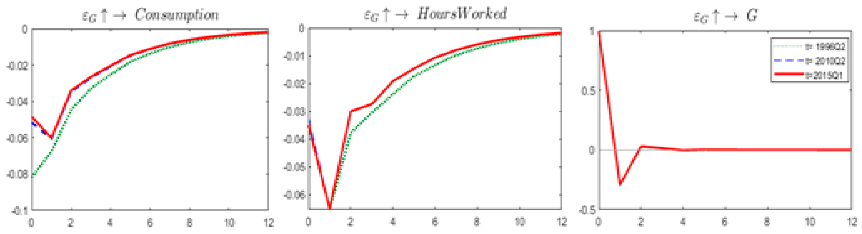
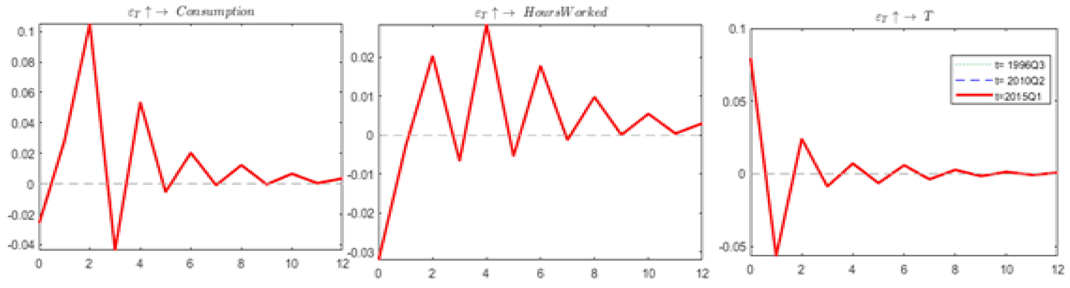
Appendix A. Impulse Responses for Alternative Sample Periods Q3 1996, Q2 2010, and Q1 2015
Figure A1.
Government expenditure shock.

Figure A2.
Tax revenue shock.

Appendix B. Alternative Specification of Priors
To check the robustness of our analysis, we also assumed priors such as where and G represent the inverse Wishart and gamma distributions and and are the diagonal elements in and , respectively.
Figure A3.
Government expenditure shock.

Figure A4.
Tax revenue shock.

References
- Afonso, Antonio. 2008. Ricardian fiscal regimes in the European Union. Empirica 35: 313–34. [Google Scholar] [CrossRef]
- Amano, Robert A., and Tony S. Wirjanto. 1998. Government Expenditures and the Permanent—Income Model. Review of Economic Dynamics 1: 719–30. [Google Scholar] [CrossRef]
- Ambler, Steve, and Alain Paquet. 1996. Fiscal Spending Shocks, Endogenous Government Spending, and Real Business Cycles. Journal of Economic Dynamics and Control 20: 237–56. [Google Scholar] [CrossRef]
- Aschauer, David. 1985. Fiscal Policy and Aggregate Demand. American Economic Review 75: 117–27. [Google Scholar]
- Auerbach, Alan J., and Yuriy Gorodnichenko. 2012. Fiscal Multipliers in Recession and Expansion. In Fiscal Policy after the Financial Crisis. NBER Chapters. Cambridge: National Bureau of Economic Research, Inc., p. 63. [Google Scholar]
- Bachmann, Rudier, and Eric R. Sims. 2012. Confidence and the transmission of government spending shocks. Journal of Monetary Economics 59: 235–49. [Google Scholar] [CrossRef]
- Baum, Anja, Marcos Poplawski-Ribeiro, and Anke Weber. 2012. Fiscal Multipliers and the State of the Economy. IMF Working Papers 12/286. Washington, DC: International Monetary Fund. [Google Scholar]
- Baumeister, Christiane, Eveline John Durinck, and Gert Peersman. 2008. Liquidity, Inflation and Asset Prices in a Time-Varying Framework for the Euro Area. National Bank of Belgium Working Paper 142. Belgium: National Bank. [Google Scholar]
- Baxter, Marianne, and Robert G. King. 1993. Fiscal Policy in General Equilibrium. American Economic Review 83: 315–34. [Google Scholar]
- Benati, Luca. 2008. Investigating Inflation Persistence across Monetary Regimes. The Quarterly Journal of Economics 123: 1005–60. [Google Scholar] [CrossRef]
- Black, Fisher. 1976. Studies of stock price volatility changes. In Proceedings of the Business and Economic Statistics Section. Washington, DC: American Statistical Association, pp. 177–81. [Google Scholar]
- Blanchard, Olivier, and Roberto Perotti. 2002. An empirical characterization of the dynamic effects of changes in government spending and taxes on output. Quarterly Journal of Economics 117: 1329–68. [Google Scholar] [CrossRef]
- Burnside, Craig, Martin Eichenbaum, and Jonas D. M. Fischer. 1998. Assessing the Effects of Fiscal Shocks. Working Paper 7459. Cambridge: National Bureau of Economic Research, NBER. [Google Scholar]
- Canova, Fabio, and Luca Gambetti. 2009. Structural Changes in the US economy: Is There a Role for Monetary Policy? Journal of Economic Dynamics & Control 33: 477–90. [Google Scholar]
- Cimadomo, Jacopo, and Agns Benassy-Quere. 2012. Changing patterns of fiscal policy multipliers in Germany, the UK and the US. Journal of Macroeconomics 34: 845–73. [Google Scholar] [CrossRef]
- Clark, Todd E. 2011. Real-time density forecasts from Bayesian vector autoregressions with stochastic volatility. Journal of Business and Economic Statistics 29: 327–41. [Google Scholar] [CrossRef]
- Clark, Todd E., and Francesco Ravazzolo. 2015. Macroeconomic forecasting performance under alternative specifications of time-varying volatility. Journal of Applied Econometrics 30: 551–75. [Google Scholar] [CrossRef]
- Coenen, Günter, Roland Straub, and Mathias Trabandt. 2012. Fiscal policy and the Great Recession in the EA. American Economic Review 102: 71–76. [Google Scholar] [CrossRef]
- Cogan, John F., Tobias Cwik, John B. Taylor, and Volker Wieland. 2009. New Keynesian versus Old Keynesian Government Spending Multipliers. Working Paper 14782. Cambridge: National Bureau of Economic Research. [Google Scholar]
- Cogley, Timothy, and Thomas J. Sargent. 2001. Evolving Post World War II U.S. Inflation Dynamics. NBER Macroeconomics Annual 16: 331–73. [Google Scholar]
- Cogley, Timothy, and Thomas J. Sargent. 2005. Drifts and volatilities: Monetary policies and outcomes in the post WWII US. Review of Economic Dynamics 8: 262–302. [Google Scholar] [CrossRef]
- Corsetti, Giancarlo, Andre Meier, and Gernot J. Müller. 2009. Fiscal Stimulus with Spending Reversals. IMF Working Paper No 09/106. Washington, DC: International Monetary Fund, pp. 1–39. [Google Scholar]
- Crafts, Nicholas, and Terence C. Mills. 2013. Rearmament to the Rescue? New Estimates of the Impact of “Keynesian” Policies in 1930s’ Britain. The Journal of Economic History 73: 1077–104. [Google Scholar] [CrossRef]
- D’Agostino, Antonello, Luca Gambetti, and Domenico Giannone. 2013. Macroeconomic forecasting and structural change. Journal of Applied Econometrics 28: 82–101. [Google Scholar] [CrossRef]
- DeLong, Bradford, and Lawrence Summers. 2012. Fiscal Policy in Depressed Economy. Brookings, March 20. [Google Scholar]
- Edelberg, Wendy, Martin Eichenbaum, and Jonas D. M. Fisher. 1999. Understanding the Effects of Shocks to Government Purchases. Review of Economic Dynamics 2: 166–206. [Google Scholar] [CrossRef]
- Ellis, Colin, Haroon Mumtaz, and Pawel Zabczyk. 2014. What Lies Beneath? A Time-varying FAVAR Model for the UK Transmission Mechanism. The Economic Journal 124: 668–99. [Google Scholar] [CrossRef]
- Enders, Zeno, Gernot Müller, and Almuth Scholl. 2008. How Do Fiscal and Technology Shocks Affect Real Exchange Rates? New Evidence for the United States. No. 2008/22. Frankfurt: Center of Financial Studies. [Google Scholar]
- Farmer, Roger E., and Dmitry Plotnikov. 2012. Does fiscal policy matter? Blinder and Solow revisited. Macroeconomic Dynamics 16: 146–66. [Google Scholar] [CrossRef]
- Fatas, Antonio, and Ilian Mihov. 2001. Fiscal Policy and Business Cycles: An Empirical Investigation. Working Paper-INSEAD R and D. Paris: INSEAD. [Google Scholar]
- Forni, Lorenzo, Libero Monteforte, and Luca Sessa. 2009. The general equilibrium effects of fisscal policy: Estimates for the Euro area. Journal of Public Economics 93: 559–85. [Google Scholar] [CrossRef]
- Galí, Jordi, J. David López-Salido, and Javier Vallés. 2007. Understanding the Effects of Government Spending on Consumption. Journal of the European Economic Association 5: 227–70. [Google Scholar] [CrossRef]
- Geweke, John. 1992. Evaluating the Accuracy of Sampling-Based Approaches to the Calculation of Posterior Moments. In Bayesian Statistics. Edited by José-Miguel Bernardo, J. O. Berger, Philip A. Dawid and Adrian F. M. Smith. New York: Oxford University Press, Volume 4, pp. 169–88. [Google Scholar]
- Ghysels, Eric, Andrew C. Harvey, and Eric Renault. 1996. Stochastic volatility. In Handbook of Statistics, Statistical Method in Finance. Edited by Gangadharrao S. Maddala. Amsterdam: Elsevier, vol. 14, p. 119. [Google Scholar]
- Glocker, Christian, Giulia Sestieri, and Pascal Towbin. 2017. Time-Varying FISCAL Spending Multipliers in the UK. Working Papers 643. Paris: Banque de France. [Google Scholar]
- Hall, Robert E. 1986. The Role of Consumption in Economic Fluctuations. In The American Business Cycle: Continuity and Change. NBER Chapters. Cambridge: NBER, pp. 237–66. [Google Scholar]
- Kapetanios, George, Haroon Mumtaz, Ibrahim Stevens, and Konstantinos Theodoridis. 2012. Assessing the Economy-Wide Effects of Quantitative Easing. No 443, Bank of England Working Papers. London: Bank of England. [Google Scholar]
- Karras, Georgios. 1994. Government Spending and Private Consumption: Some International Evidence. Journal of Money, Credit and Banking 26: 9–22. [Google Scholar] [CrossRef]
- Koop, Gary, Roberto Leon-Gonzalez, and Rodney W. Strachan. 2009. On the Evolution of the Monetary Policy Transmission Mechanism. Journal of Economic Dynamics and Control 33: 997–1017. [Google Scholar] [CrossRef]
- Kormilitsina, Anna, and Sarah Zubairy. 2016. Propagation Mechanisms for Government Spending Shocks: A Bayesian Comparison. Departmental Working Papers 1608. Dallas: Department of Economics, Southern Methodist University. [Google Scholar]
- Krugman, Paul. 2015. The Austerity Delusion. Available online: https://www.theguardian.com/business/nginteractive/2015/apr/29/the-austerity-delusion (accessed on 20 November 2018).
- Leeper, Eric M., Todd B. Walker, and Shu-Chun S. Yang. 2010. Government investment and fiscal stimulus. Journal of Monetary Economics 57: 1000–12. [Google Scholar] [CrossRef]
- Linnemann, Ludger. 2006. The Effect of Government Spending on Private Consumption: A Puzzle? Journal of Money, Credit and Banking 38: 1715–36. [Google Scholar] [CrossRef]
- Linnemann, Ludger, and Andreas Schabert. 2003. Fiscal Policy in the New Neoclassical Synthesis. Journal of Money, Credit and Banking 35: 911–29. [Google Scholar] [CrossRef]
- Mayer, Eric, Stéphane Moyen, and Nikolai Stahler. 2010. Government Expenditures and Unemployment: A DSGE Perspective. Discussion Paper/Deutsche Bundesbank/Series 1, Economic Studies 18/2010; Frankfurt: Economic Studies. [Google Scholar]
- Monacelli, Tommaso, Roberto Perotti, and Antonella Trigari. 2010. Unemployment Fiscal Multipliers Technical Report 15931. Cambridge: National Bureau of Economic Research. [Google Scholar]
- Mountford, Andrew, and Harald Uhlig. 2009. What are the effects of fiscal policy shocks? Journal of Applied Econometrics 24: 960–92. [Google Scholar] [CrossRef]
- Mumtaz, Haroon, and Laura Sunder-Plassmann. 2010. Time-Varying Dynamics of the Real Exchange Rate. A Structural VAR Analysis. Bank of England Working Papers 382. London: Bank of England. [Google Scholar]
- Nakajima, Jouchi. 2011. Time-Varying Parameter VAR Model with Stochastic Volatility: An Overview of Methodology and Empirical Applications. IMES Discussion Paper Series 11-E-09; Tokyo: Institute for Monetary and Economic Studies, Bank of Japan. [Google Scholar]
- Ni, Shawn. 1995. An Empirical Analysis on the Substitutability between Private Consumption and Government Purchases. Journal of Monetary Economics 36: 593–605. [Google Scholar] [CrossRef]
- Okubo, Masakatsu. 2003. Intratemporal Substitution between Private and Government Consumption: The Case of Japan. Economics Letters 79: 75–81. [Google Scholar] [CrossRef]
- Perotti, Roberto. 2005. Estimating the Effects of Fiscal Policy in OECD Countries. San Francisco: Federal Reserve Bank of San Francisco. [Google Scholar]
- Primiceri, Giorgio E. 2005. Time varying structural vector autoregressions and monetary policy. Review of Economic Studies 72: 821–52. [Google Scholar] [CrossRef]
- Rafiq, Sohrab. 2014. UK Fiscal multipliers in the post-war era: Do state dependent shocks matter? CESifo Economic Studies 60: 213–45. [Google Scholar] [CrossRef]
- Ramey, Valerie A., and Matthew D. Shapiro. 1998. Costly Capital Reallocation and the Effects of Government Spending. Carnegie-Rochester Conference Series on Public Policy 48: 145–94. [Google Scholar] [CrossRef]
- Ramey, Valerie A., and Sarah Zubairy. 2014. Government Spending Multipliers in Good Times and in Bad: Evidence from U.S. Historical Data. NBER Working Papers 20719. Cambridge: National Bureau of Economic Research, Inc. [Google Scholar]
- Ravn, Morten, Stephanie Schmitt-Grohé, and Martin Uribe. 2006. Deep Habits. Review of Economic Studies 73: 195–218. [Google Scholar] [CrossRef]
- Rogoff, Kenneth. 2013. Britain should not take its credit status for granted. Financial Times, October 2. [Google Scholar]
- Rotemberg, Julio J., and Michael Woodford. 1992. Oligopolistic Pricing and the Effects of Aggregate Demand on Economic Activity. Journal of Political Economy 100: 1153–207. [Google Scholar] [CrossRef]
- Shephard, Neil. 2005. Stochastic Volatility: Selected Readings. Oxford: Oxford University Press. [Google Scholar]
- Smets, Frank, and Rafael Wouters. 2007. Shocks and Frictions in US Business Cycles: A Bayesian DSGE Approach. American Economic Review 97: 586–606. [Google Scholar] [CrossRef] [Green Version]
- Taylor, John B. 2000. Reassessing Discretionary Fiscal Policy. Journal of Economic Perspectives L 14: 21–36. [Google Scholar] [CrossRef] [Green Version]
- Trichet, Jean-Claude. 2010. Reflections on the Nature of Monetary Policy Non Standard Measures and Finance Theory. Paper presented at Speech at the ECB Central Banking Conference, Frankfurt, Germany, November 18. [Google Scholar]
- Uhlig, Harald. 1997. Bayesian Vector Autoregressions with Stochastic Volatility. Econometrica 65: 59–73. [Google Scholar] [CrossRef]
- Yuan, Mingwei, and Wenli Li. 2000. Dynamic Employment Effects of Government Expenditure Shocks. Journal of Economic Dynamics and Control 24: 1233–63. [Google Scholar] [CrossRef]
Figure 1.
Posterior estimates for stochastic volatility.

Figure 2.
Simultaneous relationships.

Figure 3.
Impulse response functions (government expenditure shock).

Figure 4.
Impulse response functions (tax revenue shock).

Figure 5.
Impulse response functions (government expenditure shock).

Figure 6.
Impulse response functions (tax revenue shock).


Table 1.
Variable descriptions.
| Variable | Description |
|---|---|
| Government expenditure | Government consumption expenditure, gross fixed capital formation, social payments, other payables Source: Eurostat database |
| Net tax revenue | Direct taxes: income tax, wealth tax, corporate tax; indirect taxes: value-added tax (VAT) and taxes on production and imports Source: Eurostat database |
| Private consumption | Household final consumption expenditure Source: Office for National Statistics |
| Weekly hours worked | Estimates of mean actual hours of work including overtime per week Source: Office for National Statistics |
Table 2.
Estimation results of time-varying parameter vector autoregression (TVP-VAR) and Markov chain Monte Carlo (MCMC) convergence diagnostics.
Table 2.
Estimation results of time-varying parameter vector autoregression (TVP-VAR) and Markov chain Monte Carlo (MCMC) convergence diagnostics.
| Parameter | Mean | Std Dev | 95% Interval | Geweke Convergence Diagnostics | Inefficiency |
|---|---|---|---|---|---|
| 0.0023 | 0.0003 | (0.0018, 0.0029) | 0.881 | 5.94 | |
| 0.0023 | 0.0003 | (0.0018, 0.0029) | 0.716 | 7.22 | |
| 0.0056 | 0.0016 | (0.0033, 0.0094) | 0.657 | 31 | |
| 0.0056 | 0.0019 | (0.0034, 0.0107) | 0.307 | 43.65 | |
| 0.0059 | 0.0018 | (0.0034, 0.0102) | 0.924 | 52.48 | |
| 0.1674 | 0.0458 | (0.0921, 0.2723) | 0.671 | 46.02 |
Table 3.
Sign restrictions in case of expenditure and tax shock.
| Variable | Restriction |
|---|---|
| Private consumption (C) | - |
| Average weekly hours worked (W) | + |
| Government expenditure (G) | + |
© 2019 by the author. Licensee MDPI, Basel, Switzerland. This article is an open access article distributed under the terms and conditions of the Creative Commons Attribution (CC BY) license (http://creativecommons.org/licenses/by/4.0/).
Share and Cite
MDPI and ACS Style
Shaheen, R. Impact of Fiscal Policy on Consumption and Labor Supply under a Time-Varying Structural VAR Model. Economies 2019, 7, 57. https://0-doi-org.brum.beds.ac.uk/10.3390/economies7020057
AMA Style
Shaheen R. Impact of Fiscal Policy on Consumption and Labor Supply under a Time-Varying Structural VAR Model. Economies. 2019; 7(2):57. https://0-doi-org.brum.beds.ac.uk/10.3390/economies7020057
Chicago/Turabian StyleShaheen, Rozina. 2019. "Impact of Fiscal Policy on Consumption and Labor Supply under a Time-Varying Structural VAR Model" Economies 7, no. 2: 57. https://0-doi-org.brum.beds.ac.uk/10.3390/economies7020057
Note that from the first issue of 2016, this journal uses article numbers instead of page numbers. See further details here.