The Impact of International Sanctions on Russian Financial Markets

Abstract

Russia’s international comportment and geostrategic moves, particularly the invasion of Ukraine and the annexation of Crimea in 2014, caused a substantial change in its international economic and political relations. In response to Russia’s invasion, the United States of America, the European Union, and their allies imposed a series of sanctions. In this study, by applying an exponential generalized autoregressive conditional heteroscedasticity model to daily logarithmic returns of the ruble exchange rate and the closing price index of the Russian Trading System, we analyze how the returns and volatility of the exchange rate and the stock price index responded to the sanctions and oil price changes. The estimation results show that the sanctions have a significant positive short-term impact on exchange rate returns. Economic sanctions have a significant negative long-term impact on the returns and variance of the exchange rate and a significant positive long-term impact on the returns of the stock price index. Financial sanctions have a positive/negative long-term impact on the returns of the exchange rate/stock price index and a positive long-term impact on the variance of the exchange rate and the stock price index. Corporate sanctions have a positive long-term impact on exchange rate returns.

1. Introduction

Russia’s international comportment and geostrategic moves, particularly the invasion of Ukraine and the annexation of Crimea between February and March 2014, caused a substantial change in its international economic and political relations. In response to Russia’s invasion, the United States of America (US), the European Union (EU), and their allies imposed a series of sanctions. A total of 15 economic, 12 financial and 22 corporate sanctions on Russia were applied by the US and the EU between 3 March 2014 and 13 September 2018 (Radio Free Europe/Radio Liberty 2018). During the same period, five diplomatic and 31 personal sanctions were imposed, and previous sanctions were extended 21 times. Except for one sanction related to the war in Syria, two sanctions related to the Russian presidential elections and three sanctions related to the Sergei Skripal incident in 2018 (on 4 March, Sergei Skripal, a former Russian military officer, and his daughter were poisoned in the city of Salisbury, England), all other sanctions were linked to Ukraine. As a response to the sanctions, Russia banned imports of certain foodstuffs from the EU and further enhanced its long-term import substitution policy aimed at economic sovereignty and ensuring the supply of important products, which had been the focus since the early 2000s. The government also approved the “Government Program on Industries and Competitiveness” to bolster domestic production in almost all industries (Korhonen et al. 2018).

The Council of the EU justified the sanctions as a response to the illegal annexation of Crimea and Sevastopol and Russia’s destabilizing actions in Ukraine (Council of the European Union 2014). The US Congress cited the sanctions as support for the sovereignty, integrity, democracy and economic stability of Ukraine and condemnation of the unjustified military intervention of Russia in the Crimea region and its occupation, as well as any other form of political, economic or military aggression against Ukraine (United States Congress 2014).

In the opposite camp, Western sanctions were seen as acts of aggression against Russian interests. Yevgeniy Primakov, a distinguished Russian politician and diplomat, interpreted the Crimea-related conflicts and sanctions as attempts by the US to promote the establishment of military control over the Black Sea within the frame of US policy, aimed at establishing a unipolar world order and pushing Russia out of world politics (Primakov 2015). Rustem Nureev, a representative of Russian academia, divided the reasons for the sanctions against Russia into geopolitical and economic, such as attempts to weaken Russia’s position on major international issues and limit Russian companies’ competitiveness in the global market and especially in the European market (Nureev 2017).

Coincidentally, in July 2014, the price of crude oil began to fall in the international energy market. The price of WTI/Brent fell from 106.1/110.1 USD on 1 July 2014 to 56.9/61.7 USD on 1 July 2015 and to 32.1/30.1 USD on 22 January 2016 (as reported by Thomson Reuters). As a result, fuel exports as a percentage of Russian merchandise exports decreased from 71.2% in 2013 to 48.2% in 2016 (World Bank 2020a).

This external shock generated by the imposed sanctions and the low oil price had a considerable impact on the Russian economy. The Russian currency’s exchange rate depreciated from 33.8 rubles per 1 USD on 1 July 2014 to 55.8 rubles on 1 July 2015 and to 83.6 rubles on 22 January 2016 (Central Bank of Russia 2020). Exports of goods and services decreased from 592 billion USD in 2013 to 562.5 billion in 2014 and to 393 billion in 2015. Imports decreased from 470 billion USD in 2013 to 429 billion in 2014 and to 282 billion in 2015 (World Bank 2020b, 2020c).

Massive devaluation of the ruble required a change in exchange rate policy and proper measures to stabilize the financial system. The Central Bank of Russia spent 30 billion USD to support the exchange rate of the ruble in October 2014. A month later, the central bank shifted to a free-floating exchange rate to avoid further depletion of reserves. Further measures to enhance financial policy were taken in December 2014. In particular, the central bank introduced foreign currency loans to the 11 banks with large capital, major state-owned exporters were required to cut their net foreign assets, a one-trillion rubles bank recapitalization program was launched through the issuance of treasury bonds, and a bill allowing the government to invest 10% of the National Wealth Fund in deposits and bank bonds was approved (World Bank 2015).

In this study, applying an exponential generalized autoregressive conditional heteroscedasticity (EGARCH) model to daily logarithmic returns of the ruble exchange rate and closing price index of the Russian Trading System (RTS), we analyze how the returns and volatility of the exchange rate and the stock price index responded to the sanctions and the oil price decline.

While the impact of the oil price on Russian financial markets is widely addressed in the literature, the impact of economic sanctions is less analyzed. Researchers have used various approaches to assess the impact of sanctions on Russian financial markets. Comparison of changes in and between financial variables in different periods before and after sanctions were imposed (Schmıdbauer et al. 2016; Tyll et al. 2018), use of a general index including all types of sanctions with different weights (Dreger et al. 2015; Kholodilin and Netšunajev 2019), and the incorporation of separate dummy variables for each sanction while researching the impact of a limited number of sanctions (Stone 2017). The application of the EGARCH model, the use of high-frequency daily data and the incorporation of economic, financial, and corporate sanctions as separate dummy variables in return and variance equations enable us to aptly assess the sanctions’ impact on the returns and volatility of essential variables of Russian financial markets. Incorporating dummy variables for the days of the first two weeks following the days on which sanctions were announced and ordinal dummy variables for the periods after the days on which sanctions were announced, we measure both short- and long-term impacts of sanctions.

This paper is organized as follows. In the next section, we review the research findings of the related literature. The data and methodology used in our estimations are described in Section 3. In Section 4, we present the estimation results. Section 5 concludes the paper.

2. Literature Review

International sanctions became a familiar attribute of international relations in the twentieth century. The League of Nations and its successor, the United Nations (UN), institutionalized international sanctions as norms of behavior to promote the peaceful settlement of international disputes (Doxey 1987).

The effectiveness of international sanctions is assessed by their contribution to achieving changes in the policies enacted by the target country. Early empirical research, such as Galtung’s (1967) and Lindsay’s (1986), described international sanctions as ineffective tools in international relations, while Hufbauer et al. (1990), assessing 116 sanctions for the period 1914 to 1990, found that 34% of the sanctions were effective. Weber and Schneider (2020) integrated and amended the existing sanctions databases and counted 326 sanction threats and imposed sanctions by the EU, the US, and the UN for the period of 1989 to 2015. The US imposed 182 sanctions against 103 countries, including 119 cases individually imposed and 63 cases imposed with the EU or the UN. The EU imposed 81 sanctions against 60 countries, including 10 cases imposed individually and 71 cases imposed together with the US or the UN. The UN imposed 34 sanctions against 29 countries, including five cases imposed individually and 29 cases imposed with the US or the EU. Research results (Weber and Schneider 2020) reveal partial effectiveness for the imposed sanctions in the period 1989 to 2015, similar to Hufbauer et al. (1990), and show that sanctions by the EU and the UN were more successful compared to those imposed by the US. Jing et al. (2003) and Smeets (2018), examining related studies, demonstrate that despite significant economic and social impacts, the effectiveness of international sanctions is arguable (Smeets 2018); the relationship between the imposing country and the targeted country, as well as targeted countries’ economic and political strength, are important factors affecting the practicality of the imposed sanctions (Jing et al. 2003).

Few studies have assessed the impact of sanctions on Russian financial markets. Dreger et al. (2015), based on cointegrated vector autoregressive (VAR) models and daily data for the period from 1 January 2014 to 31 March 2015, claim that the depreciation of the ruble may be related to the decline of oil prices, while the sanctions affected only the conditional volatility of the exchange rate. Schmıdbauer et al. (2016), using a VAR model in daily returns for six representative stock markets (of the US, the UK, the EU, Japan, China, and Russia) from 3 March 1998 to 6 July 2015, argue that the sanctions reduced the importance of the Russian stock market as a propagator of return shocks but increased its significance as a propagator of volatility shocks in international financial markets. Applying a generalized autoregressive conditional heteroscedasticity (GARCH) model to data for the period between 1 January 2014 and 31 October 2014, Stone (2017) demonstrates that the flow of information on sanctions is associated with a decrease in the returns and an increase in the variance of Russian securities. Tyll et al. (2018), applying an autoregressive distributed lag model and dynamic least squares to daily data for the period from 2 January 2013 to 7 November 2016, provide statistically confirmed evidence that the sanctions have rendered the exchange rate of the ruble firmly bound to oil price changes. Kholodilin and Netšunajev (2019), using a structural VAR model and quarterly data for 1997 Q1–2018 Q1, show that the real effective exchange rate of the ruble depreciated following the sanction shock. They explain the impact of the sanctions on the exchange rate as a consequence of changes in foreign trade caused by the sanctions.

The sanctions coincided with a considerable fall in the price of oil in the international energy market and the consequent decrease in income from fuel exports. Hence, studies assessing the sanctions’ impact have considered the decline in oil prices an essential factor behind the economic deterioration (Dreger et al. 2015; Tyll et al. 2018). Given Russia’s heavy dependence on commodity exports, imports of consumer goods, and foreign investment, researchers anticipated a substantial impact of the oil price decline and the sanctions on the country’s economy (Dreger et al. 2015; Tyll et al. 2018; Kholodilin and Netšunajev 2019).

3. Data and Methodology

3.1. Data Description

The sanction data used in our estimations are displayed in

Table 1. Sanctions Imposed on Russia by the US and the EU.

Sanctions	2014	2015	2016	2017	2018
Economic	US 8	US 2	US 0	US 0	US 1
	EU 4	EU 0	EU 0	EU 0	EU 0
Financial	US 5	US 1	US 0	US 0	US 1
	EU 5	EU 0	EU 0	EU 0	EU 0
Corporate	US 5	US 3	US 4	US 1	US 2
	EU 4	EU 1	EU 0	EU 1	EU 1

Source: The information is based on original data from Radio Free Europe/Radio Liberty (2018). Notes: The numbers after US and EU denote the number of sanctions that each imposed. Abbreviations: US—United States of America, EU—European Union.

. During the period covered in our analysis, a total of 49 economic, financial and corporate sanctions were imposed on Russia by the US and the EU. Economic sanctions include measures such as trade suspension, export and import restrictions, and restrictions on the export of various oil and gas technologies. Suspension of trade and investment talks and military-to-military cooperation with Russia (by the US), the ban on the issuance of export licenses for defense products and services to Russia (by the US), restriction of import of goods deemed to contribute to Russian military capability (by the US), sanctions on defense-related Russian companies and partial ban on investment in Crimea (by the EU), restrictions on the export of oil and gas goods and technologies to Russia (by the US) and a ban on trade with Crimea (by the US and the EU) are real examples of economic sanctions. Financial sanctions are those specifically targeting Russian banks and financial institutions. Examples include the restriction of access to capital markets for the Bank of Moscow, Bank Rossia, Gazprombank, the Russian Agricultural Bank, the Russian National Commercial Bank, Sberbank, Vneshekonombank and VTB Bank. Corporate sanctions include the suspension of financing for Russian companies and their inclusion in the sanctions list. The list included Crimean energy companies (Chernomorneftegaz and Feodosia), Russian key energy companies (Novatek, Rosneft, Transneft, Gazpromneft, and Uralvagonzavod), Russian military and defense companies (Oboronprom, United Aircraft Corporation, and Almaz-Antey) and companies believed to be linked to President Vladimir Putin.

Descriptive statistics for daily logarithmic return series of the exchange rate, stock price index and crude oil prices during the period 29 January 2014–19 September 2018 are presented in

Table 2. Descriptive Statistics.

Variables	Mean	SD	Skewness	Kurtosis	ARCH LM	ADF
Ruble	0.00062	0.01421	0.41435	17.5496	224.263 ***	−4.49400 ***
RTS	−0.00015	0.01979	−0.49856	10.8321	148.697 ***	−6.64800 ***
WTI	−0.00029	0.02489	−0.49078	9.24029	11.0290 ***	−6.34300 ***
Brent	−0.00030	0.02306	−0.93690	15.6977	2.07200	−6.44800 ***

Source: The exchange rate data are from the Central Bank of Russia. The stock price index data are from the Moscow Exchange. The crude oil prices are from Thomson Reuters. Notes: The maximum number of lags for the augmented Dickey-Fuller (ADF) test selected by the Schwarz information criterion was 21. *** indicates statistical significance at the 1% significance level. The total number of observations is 1074. Weekends and holidays are excluded. Abbreviations: SD—standard deviation, ARCH—autoregressive conditional heteroscedasticity, LM—Lagrange multiplier, ADF—augmented Dickey-Fuller.

.

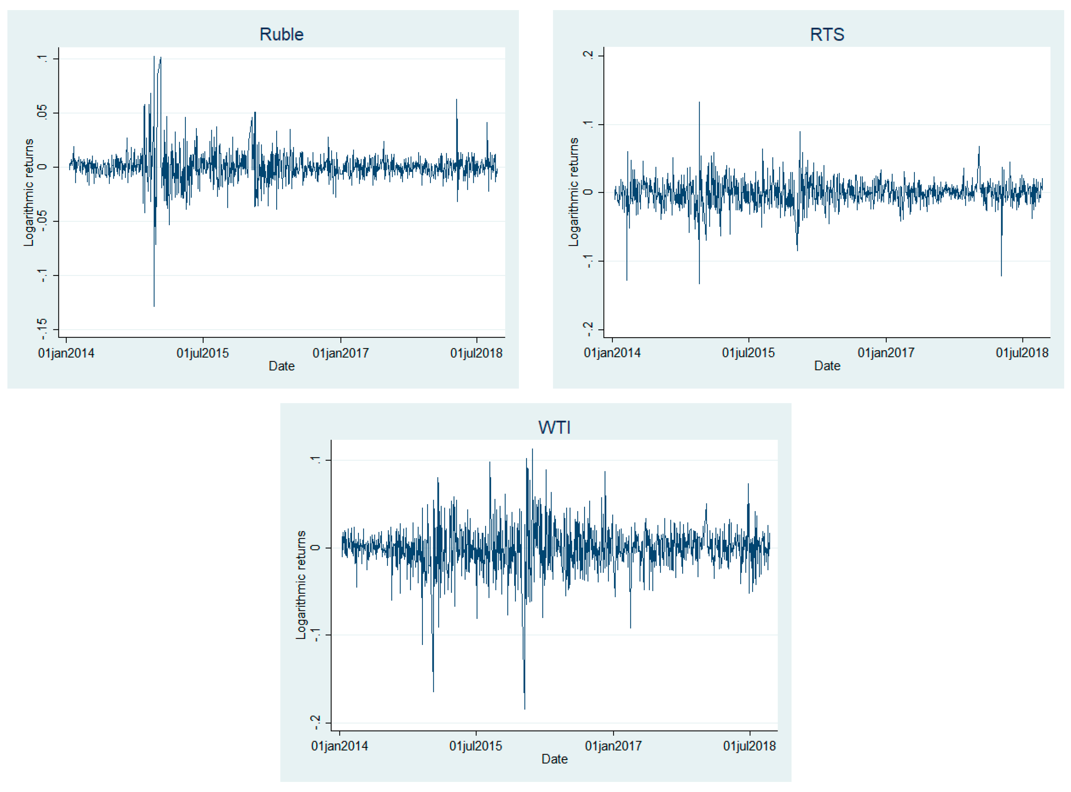
The mean values indicate an increasing trend for the ruble and a decreasing trend for other variables. The standard deviation values show higher volatility for crude oil. The skewness and kurtosis values show that the data are not normally distributed. Logarithmic returns are leptokurtic for all variables, with a positive skew for the ruble and a negative skew for other variables.

At a 1% significance level, the Lagrange multiplier test for autoregressive conditional heteroscedasticity (ARCH) rejects the null hypothesis that the errors are not autoregressive conditional heteroskedastic for all variables except Brent. Considering the absence of an ARCH effect, we exclude Brent from further estimations. According to the augmented Dickey-Fuller test (Dickey and Fuller 1979, 1981) for unit root, the time series are stationary. The test statistics are smaller than the critical values at a 1% significance level.

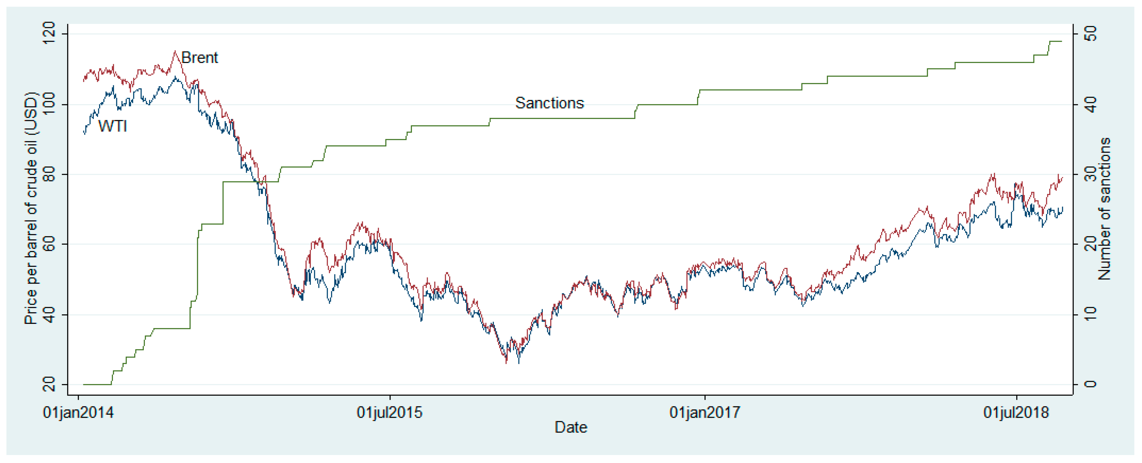
The logarithmic return series used in our estimations are illustrated in Figure 1. The illustrations support the descriptions of the statistics displayed in Table 2. Additionally, Figure 1 shows that the series are more volatile in the first than in the second half of the period in question. This may be explained by comparing the logarithmic return series in Figure 1 to the original data (levels) in Figure A1 and Figure A2 in Appendix A. As shown in Figure A1 and Figure A2, most sanctions were announced in the first half of the period in question. A sharp decline in crude oil prices also occurred in the first half of that period. The sanction announcements and drop in the crude oil price seem to be associated with a massive depreciation of the exchange rate and a substantial change in the stock price index.

3.2. Methodology

Referring to a huge number of empirical studies, Bollerslev et al. (1992) demonstrated that ARCH models are more suitable for analysis of the time-varying volatility of financial data than other econometric models. The original ARCH stochastic processes introduced by Engle (1982) are mean-zero, serially-uncorrelated processes with nonconstant variances conditional on past constant unconditional variances in which the recent past provides information about the one-period forecast variance. The model suggested by Engle (1982) was further developed for the generalized ARCH (GARCH) by Bollerslev (1986), the absolute error model by Taylor (1986) and Schwert (1989), the exponential GARCH (EGARCH) by Nelson (1991), and the GJR (Glosten, Jagannathan, and Runkle) model by Glosten et al. (1993).

The original model is given by

$${\mathrm{y}}_t=c+b{x}_t+{\epsilon }_t,$$

(1)

where $y_t$ is the dependent variable, $c$ is a constant, $b$ is a vector of unknown parameters, $x_t$ is a vector of explanatory variables, $\epsilon$ represents innovations denoting a real-valued discrete-time stochastic process and t is time. Given the information set of all information (${\phi }_t$) through time t, Bollerslev’s GARCH process is

$$\begin{array}{c}{\epsilon }_t|{\phi }_{t-1}~\mathrm{N}(0,h_t),\\ h_t=\omega +{\sum }_{i=1}^p{\alpha }_i{\epsilon }_{t-i}^2+{\sum }_{i=1}^q{\beta }_i{h}_{t-i},\end{array}$$

(2)

where $\omega >0,{\alpha }_i\ge 0\left(i=1,\dots ,p\right),p>0,{\beta }_i\ge 0\left(i=1,\dots ,q\right),q\ge 0.$ The natural generalization of the ARCH process proposed by Bollerslev (1986) allows for past conditional variances to enter the current conditional variance equation.

Nelson (1991) argued that the dynamics of GARCH models are unduly restrictive and frequently violated by estimated coefficients. Hence, he proposed an EGARCH model, where the log value of volatility is used as an explained variable and no sign constraints on parameters of variance dynamics are imposed. The variance equation of EGARCH is

$$ln{h}_t=\omega +{\displaystyle \sum }_{i =1}^p\{{\gamma }_i\left({\epsilon }_{t-i}/h_{t-i}^{1/2}\right)+{\alpha }_i(|{\epsilon }_{t-i}/h_{t-i}^{1/2}|)\}+{\displaystyle \sum }_{i =1}^q{\beta }_{i}ln{h}_{t-i},$$

(3)

where ${\gamma }_i$, ${\alpha }_i$, and ${\beta }_i$ are the asymmetric effect of information about past volatility, the symmetric effect of information about past volatility and volatility persistence, respectively.

We model the logarithmic returns of the ruble exchange rate and the stock price index as a function of their prior returns, prior oil price returns and dummy variables for sanctions (Equation (1) with dummy variables). The log values of variances are modeled as a function of the previous periods’ standardized information, the log value of variance, oil price returns and dummy variables for sanctions (Equation (3) with dummy variables).

The parameters of the model (the number of lags for dependent variables included in the returns equation (Equation (1)) and the number of lags for information (p) and past variances (q) in the variance equation (Equation (3)) are determined based on information criteria and standardized residuals diagnostic results.

Dummy variables for measuring the short-term impact of sanctions take a value of 1 for the days of the first two weeks following the days on which sanctions are announced and 0 for all other days. Ordinal dummy variables for measuring the long-term impact of sanctions are used. These dummy variables take a value of 0 before and a value of 1 after the days on which sanctions are announced. We solve Equations (1) and (3) with one dummy variable for all economic, financial, and corporate sanctions combined (Model 1 for short-term impacts and Model 3 for long-term impacts) and with three separate dummy variables for economic, financial, and corporate sanctions (Model 2 for short-term impacts and Model 4 for long-term impacts). By incorporating separate dummies for each sanction, we were able to get more informative results. However, the number of equations to be estimated increases, and for most of the equations, diagnostic tests do not support the estimation results.

Since Russia is one of the main exporters of oil, sanctions imposed on Russia might affect oil prices as well. Nonetheless, the coincidence of sanctions with a period of a sharp fall in the price of crude oil caused by changes in demand and supply in the international energy market makes the impact of sanctions on crude oil price insignificant.

4. Empirical Findings

4.1. Short-Term Impact of Sanctions

Application of the GARCH model (combination of Equations (1) and (2)) showed that the restrictions were violated by estimated coefficients, as mentioned in Nelson (1991). The sign of the constant was negative for all equations, affecting the reliability of estimation results negatively (

Table A1. GARCH Model Estimations of the Short-Term Impact of Sanctions.

	Exchange Rate Logarithmic Returns (Ruble)		Stock Price Index Logarithmic Returns (RTS)
	Model 1	Model 2	Model 1	Model 2
Mean equation
$y_{t-1}$	0.0314 (0.0308)	0.0291 (0.0307)	0.0077 (0.0339)	0.0067 (0.0342)
$y_{t-2}$	−0.0071 (0.0305)	−0.0080 (0.0299)
$y_{t-3}$	−0.0664 ** (0.0310)	−0.0682 ** (0.0309)
$WT{I}_{t-1}$	−0.0420 *** (0.0134)	−0.0409 *** (0.0131)	0.0757 *** (0.0247)	0.0766 *** (0.0247)
Sanction dummy
All	0.0003 * (0.0001)		−0.0003 (0.0004)
Economic		0.0012 (0.0011)		0.0008 (0.0024)
Financial		0.0005 (0.0011)		−0.0014 (0.0020)
Corporate		−0.0010 ** (0.0005)		−0.0003 (0.0011)
$c$	0.0001 (0.0003)	0.0003 (0.0003)	0.0003 (0.0005)	0.0002 (0.0005)
Variance equation
${\alpha }_1$	0.2418 *** (0.0771)	0.2490 *** (0.0796)	0.0448 *** (0.0156)	0.0443 *** (0.0153)
${\alpha }_2$	−0.1586 * (0.0829)	−0.1584 ** (0.0800)
${\beta }_1$	0.9002 *** (0.0436)	0.8893 *** (0.0340)	0.9419 *** (0.0180)	0.9427 *** (0.0174)
$WT{I}_{t-1}$	34.6010 ** (17.6391)	35.0140 ** (13.9890)	−29.8911 *** (4.0547)	−32.4463 *** (9.3880)
Sanction dummy
All	−0.0041 (0.1558)		0.0578 (0.2011)
Economic		−4.1096 ** (1.9771)		−0.3556 (1.2357)
Financial		2.2812 *** (0.6123)		0.6020(1.3912)
Corporate		0.1225 (0.4235)		−0.3278 (1.2867)
$\omega$	−13.2686 *** (0.6430)	−13.1121 *** (0.5508)	−12.7489 *** (0.6241)	−12.7487 *** (0.6228)
Portmanteau (Q) statistic, lags (5)
Standardized residuals	5.2971 (0.3807)	5.0564 (0.4090)	2.3588 (0.7976)	2.4653 (0.7817)
Standardized residuals (squared)	1.0890 (0.9551)	0.8887 (0.9710)	1.1713 (0.9476)	1.1225 (0.9521)

Notes: The numbers in parentheses are standard errors. *, **, and *** indicate significance at the 10%, 5%, and 1% levels, respectively.

and

Table A2. GARCH Model Estimations of the Long-Term Impact of Sanctions.

	Exchange Rate Logarithmic Returns (Ruble)		Stock Price Index Logarithmic Returns (RTS)
	Model 1	Model 2	Model 1	Model 2
Mean equation
$y_{t-1}$	0.0319 (0.0309)	0.0304 (0.0312)	0.0083 (0.0337)	0.0082 (0.0339)
$y_{t-2}$	−0.0043 (0.0303)	−0.0136 (0.0304)
$y_{t-3}$	−0.0648 ** (0.0308)	−0.0718 ** (0.0311)
$WT{I}_{t-1}$	−0.0423 *** (0.0132)	−0.0386 *** (0.0136)	0.0761 *** (0.0246)	0.0738 *** (0.0249)
Sanction dummy
All	−2.6 × 10−5 (−1.7 × 10−5)		−4.6 × 10−5 (−3.7 × 10−5)
Economic		−0.0010 ** (0.0004)		0.0014 * (0.0008)
Financial		0.0011 ** (0.0005)		−0.0016 * (0.0009)
Corporate		−1.5 × 10−5 (0.0001)		−4.7 × 10−5 (0.0002)
$c$	0.0012 * (0.0007)	0.0007 (0.0008)	−0.0016 (0.0015)	−0.0009 (0.0017)
Variance equation
${\alpha }_1$	0.2538 *** (0.0803)	0.2239 *** (0.0769)	0.0435 *** (0.0147)	0.0361 *** (0.0127)
${\alpha }_2$	−0.1679 ** (0.0855)	−0.1323 (0.0818)
${\beta }_1$	0.8974 *** (0.0443)	0.8729 *** (0.0572)	0.9364 *** (0.0186)	0.9379 *** (0.0200)
$WT{I}_{t-1}$
Sanction dummy	36.2570 ** (14.9062)	33.7129 *** (9.8200)	−29.9437 *** (3.1247)	−26.3059 *** (4.3985)
All
Economic	−0.0042 (0.0096)		−0.0238 ** (0.0108)
Financial		−0.1272 (0.2216)		−0.1769 (0.2116)
Corporate		0.3305 (0.2357)		0.3398 (0.2412)
$\omega$		−0.0934 (0.0583)		−0.0978 (0.0644)
Portmanteau (Q) statistic, lags (5)
Standardized residuals	5.4528 (0.3632)	3.7706 (0.5829)	2.7245 (0.7424)	2.3909 (0.7928)
Standardized residuals (squared)	0.8988 (0.9703)	0.6960 (0.9832)	1.1098 (0.9532)	0.6692 (0.9846)

Notes: The numbers in parentheses are standard errors. *, **, and *** indicate significance at the 10%, 5%, and 1% levels, respectively.

in Appendix A). Therefore, we applied the EGARCH model (combination of Equations (1) and (3) (

Table 3. EGARCH Model Estimations of the Short-Term Impact of Sanctions.

	Exchange Rate Logarithmic Returns (Ruble)			Stock Price Index Logarithmic Returns (RTS)
	Model 0	Model 1	Model 2	Model 0	Model 1	Model 2
Mean equation
$y_{t-1}$	0.0306 *** (0.0110)	0.0177 (0.0316)	0.0222 (0.0452)	0.0472 (0.0302)	0.0054 (0.0319)	0.0069 (0.0343)
$WT{I}_{t-1}$		−0.0388 *** (0.0139)	−0.0386 *** (0.0148)		0.0827 *** (0.0236)	0.0829 *** (0.0250)
Sanction dummy
All		0.0003 *** (3.06 × 10−5)			−0.0004 (0.0004)
Economic			0.0017 (0.0033)			0.0010 (0.0022)
Financial			−0.0001 (0.0032)			−0.0014 (0.0019)
Corporate			−0.0009 (0.0011)			−0.0006 (0.0012)
$c$	0.0003 ** (0.0001)	0.0001 (0.0002)	0.0002 (0.0004)	−2.15×10−5 (0.0004)	0.0001 (0.0005)	0.0001 (0.0005)
Variance equation
${\gamma }_1$	0.0887 *** (0.0231)	0.0913 *** (0.0305)	0.0950 *** (0.0309)	−0.0697 *** (0.0171)	−0.0640 *** (0.0203)	−0.0666 *** (0.0212)
${\alpha }_1$	0.2167 *** (0.0602)	0.2113 *** (0.0684)	0.1980 ** (0.0836)	0.1036 *** (0.0210)	0.0954 *** (0.0213)	0.0977 *** (0.0217)
${\beta }_1$	0.9758 *** (0.0122)	0.9750 *** (0.0148)	0.9810 *** (0.0158)	0.9870 *** (0.0050)	0.9875 *** (0.0047)	0.9879 *** (0.0049)
$WT{I}_{t-1}$		0.1284 (1.6477)	−0.1593 (1.7934)		−0.8046 (0.9038)	−0.7817 (0.9732)
Sanction dummy
All		−0.0031 (0.0066)			−0.0014 (0.0033)
Economic			−0.0432 (0.0541)			−0.0104 (0.0221)
Financial			0.0170 (0.0503)			−0.0016 (0.0207)
Corporate			0.0209 (0.0313)			0.0082 (0.0147)
$\omega$	−0.2133 * (0.1092)	−0.2193 * (0.1312)	−0.1677 (0.1397)	−0.1038 *** (0.0398)	−0.1005 *** (0.0375)	−0.0974 ** (0.0393)
Portmanteau (Q) statistic, lags (5)
Standardized residuals	8.6763 (0.1227)	8.4741 (0.1320)	9.4724 (0.0916)	2.7498 (0.7385)	3.1364 (0.6790)	3.0381 (0.6941)
Standardized residuals (squared)	1.5730 (0.9045)	2.0981 (0.8354)	2.2723 (0.8103)	0.6548 (0.9854)	0.6738 (0.9844)	0.7043 (0.9827)

Notes: The numbers in parentheses are standard errors. *, **, and *** indicate significance at the 10%, 5%, and 1% levels, respectively. Sample: 29 January 2014–19 September 2018. Number of observations: 1074.

)).

The results of Equations (1) and (3) (Table 3) show a significant positive impact of one-period lagged returns of the exchange rate (at a 1% significance level) on exchange rate returns for the model without crude oil price returns and dummy variables for sanctions (Model 0). This means that appreciation/depreciation of the ruble on a given day is followed by appreciation/depreciation a day later. One-period lagged crude oil price returns have a negative/positive significant impact (at a 1% significance level) on the returns of the exchange rate/stock price index. This means that an increase/decrease in crude oil price returns on a given day is followed by an appreciation/depreciation of the ruble and an increase/decrease in the RTS returns the next day.

Given the dependence of the Russian economy on the export of energy resources, appreciation of exchange rate and the increase in stock price returns caused by a rise in the crude oil price are in line with theory.

The dummy variable for all sanctions in the first two weeks (Model 1) has a significant positive short-term impact (at a 1% significance level) on exchange rate returns. This indicates that the information about sanctions causes the exchange rate to depreciate in the first two weeks following the day on which sanctions are announced. The separate dummy variables for economic, financial, and corporate sanctions in the first two weeks (Model 2) show no significant short-term impact on exchange rate and stock price returns.

The exchange rate depreciation caused by the information about sanctions in the first two weeks is an expectable actuality as uncertainties caused by the sanctions induce investors to adjust their portfolio, selling more rubles.

The asymmetric impact of information about past volatility on conditional variance is positive/negative and statistically significant (at a 1% significance level) for the ruble/RTS. This means positive/negative information has a greater impact on future volatility of exchange rate/stock price index than negative/positive information. The symmetric impact is positive and statistically significant (at a 1–5% significance level). Previous conditional variance has a positive and statistically significant impact (at a 1% significance level) on the conditional variance of the ruble and the RTS. This fact demonstrates volatility clustering, the tendency of large changes in the exchange rate and stock price index to cluster together and result in volatility persistence.

The dummy variable for all sanctions and the separate dummy variables show no significant short-term impact on the volatility of the exchange rate and the stock price. Portmanteau (Q) statistics (Box and Pierce 1970; Ljung and Box 1978) show that there is no autocorrelation problem in standardized residuals and their squared values up to five lags, and the models are properly defined.

4.2. Long-Term Impact of Sanctions

Table 4. EGARCH Model Estimations of the Long-Term Impact of Sanctions.

	Exchange Rate Logarithmic Returns (Ruble)		Stock Price Index Logarithmic Returns (RTS)
	Model 3	Model 4	Model 3	Model 4
Mean equation
$y_{t-1}$	0.0190 (0.0392)	0.0196 (0.0179)	0.0087 (0.0337)	0.0074 (0.0349)
$WT{I}_{t-1}$	−0.0398 *** (0.0145)	−0.0360 *** (0.0084)	0.0822 *** (0.0250)	0.0795 *** (0.0254)
Sanction dummy
All	−2.02 × 10−5 (2.99 × 10−5)		3.30 × 10−5 (4.15 × 10−5)
Economic		−0.0012 *** (8.10 × 10−6)		0.0013 *** (7.61 × 10−6)
Financial		0.0014 *** (1.16 × 10−5)		−0.0016 *** (7.58 × 10−6)
Corporate		2.89 × 10−5 ** (1.18 × 10−5)		−1.28 × 10−5 (9.72 × 10−6)
$c$	0.0010 (0.0011)	0.0005 * (0.0003)	−0.0013 (0.0016)	−0.0004 *** (0.0001)
Variance equation
${\gamma }_1$	0.0917 *** (0.0323)	0.1111 *** (0.0399)	−0.0625 *** (0.0205)	−0.0771 *** (0.0228)
${\alpha }_1$	0.2195 *** (0.0723)	0.2313 *** (0.0756)	0.0962 *** (0.0219)	0.0911 *** (0.0207)
${\beta }_1$	0.9748 *** (0.0152)	0.9464 *** (0.0322)	0.9865 *** (0.0054)	0.9782 *** (0.0078)
$WT{I}_{t-1}$	0.2684 (1.6964)	1.5265 (2.0971)	−0.7297 (0.9304)	−0.1153 (1.0102)
Sanction dummy
All	5.72 × 10−5 (5.15 × 10−4)		−0.0002 (0.0003)
Economic		−0.0215 * (0.0129)		−0.0042 (0.0046)
Financial		0.0411 ** (0.0200)		0.0091 * (0.0053)
Corporate		−0.0060 (0.0061)		−0.0028 (0.0017)
$\omega$	−0.2250 (0.1385)	−0.5476 * (0.3267)	−0.1006 ** (0.0405)	−0.1789 *** (0.0629)
Portmanteau (Q) statistic, lags (5)
Standardized residuals	8.6127 (0.1255)	6.9248 (0.2263)	3.1183 (0.6818)	2.7005 (0.7460)
Standardized residuals (squared)	2.3667 (0.7964)	1.3744 (0.9271)	0.6078 (0.9876)	0.5419 (0.9905)

Notes: The numbers in parentheses are standard errors. *, **, and *** indicate significance at the 10%, 5%, and 1% levels, respectively. Sample: 29 January 2014–19 September 2018. Number of observations: 1074.

shows that the dummy variable for economic sanctions has a significant negative long-term impact (at a 1% significance level) on exchange rate returns and a significant positive long-term impact (at a 1% significance level) on RTS returns. The dummy variable for financial sanctions has a significant positive long-term impact (at a 1% significance level) on exchange rate returns and a significant negative long-term impact (at a 1% significance level) on RTS returns. The dummy variable for corporate sanctions has a significant positive long-term impact (at a 5% significance level) on exchange rate returns. The impact of the dummy variable for economic sanctions contradicts our expectations. It could be related to the anti-sanction policies taken by the Russian government. The impacts of dummy variables for financial and corporate sanctions are as expected. The dummy variable for economic sanctions has a significant negative long-term impact (at a 10% significance level) on the conditional variance of the exchange rate. The dummy variable for financial sanctions has a significant positive long-term impact on the conditional variance of the exchange rate (at a 5% significance level) and the stock price index (at a 10% significance level). This indicates the economic sanctions decreased volatility of the exchange rate, while the financial sanctions increased the volatility of the exchange rate and the stock price index.

The use of dummy variables for long-term effects instead of dummy variables for short-term effects changes, to some extent, the values and powers of all other coefficients in the estimations.

5. Concluding Remarks

In this study, applying an EGARCH model to daily logarithmic returns of the exchange rate of the ruble and closing price index of RTS, we analyzed how the returns and volatility of the exchange rate and the stock price index responded to two vital external factors, sanctions and oil price changes. The application of an EGARCH model, the use of high-frequency daily data and the incorporation of economic, financial and corporate sanctions as separate dummy variables in return and variance equations enabled us to appropriately assess the short-term and long-term impact of the sanctions on the returns and volatility of exchange rate and stock price index.

The estimation results showed that the sanctions had a significant positive short-term impact on exchange rate returns. The separation of sanctions into economic, financial and corporate and their use as dummy variables revealed no significant short-term impact on the returns and conditional variance of the exchange rate and the stock price index. Economic sanctions had a negative long-term significant impact on the returns and variance of the exchange rate and a significant positive long-term impact on the returns of the stock price index. Financial sanctions had a positive/negative long-term impact on the returns of the exchange rate/stock price index and a positive long-term impact on the variance of the exchange rate and the stock price index. Corporate sanctions had a long-term positive impact on exchange rate returns. The impact of crude oil price was negative/positive and statistically significant on exchange rate/stock price returns.

Due to the large number of sanctions assessed and the diagnostic test for estimation robustness, we were unable to incorporate separate dummy variables for each sanction as Stone (2017) had done. However, by applying an EGARCH model and incorporating economic, financial, and corporate sanctions as separate dummy variables in return and variance equations, we demonstrated the impact of sanctions on exchange rate returns, which were not revealed by Dreger et al. (2015), and assessed the difference in impact of different types of sanctions on exchange rates and stock price returns and volatility, which could not be properly demonstrated by studies using a limited number of sanctions (Stone 2017) or a general index including all types of sanctions (Dreger et al. 2015; Kholodilin and Netšunajev 2019).

Our results underscore the impact of sanctions and crude oil price on the ruble exchange rate and Russian stock price indexes and contribute to the literature on the impact of sanctions on financial markets. Furthermore, these research findings have vital importance for policy makers in decision-making and for investors who are interested in Russian financial markets for appropriate portfolio management. Precise information about differences in the short-term and long-term impact of economic, financial and corporate sanctions on returns and volatilities of exchange rate and stock price index is important for taking appropriate measures to enhance financial policy. The sanctions increase uncertainty in the financial market and the detailed information about the changes in the exchange rate and stock prices helps investors to make their decisions after sanction more rational.

References

- Bollerslev, Tim. 1986. Generalised autoregressive conditional hetroscedasticity. Journal of Econometrics 31: 307–27. [Google Scholar] [CrossRef] [Green Version]
- Bollerslev, Tim, Ray Chou, and Kenneth Kroner. 1992. ARCH modeling in finance: A review of the theory and empirical evidence. Journal of Econometrics 52: 5–59. [Google Scholar] [CrossRef]
- Box, George, and David Pierce. 1970. Distribution of residual autocorrelations in autoregressive-integrated moving average time series models. Journal of the American Statistical Association 65: 1509–26. [Google Scholar] [CrossRef]
- Central Bank of Russia. 2020. Dynamics of the Official Exchange Rates. Moscow, Russia. Available online: https://www.cbr.ru/eng/currency_base/dynamics/ (accessed on 10 May 2020).
- Council of the European Union. 2014. Council Regulation (EU) No 833/2014 of 31 July 2014 Concerning Restrictive Measures in View of Russia’s Actions Destabilising the Situation in Ukraine, Official Journal, L 229/1. pp. 1–11. Available online: http://data.europa.eu/eli/reg/2014/833/oj (accessed on 31 July 2014).
- Dickey, Alan, and Arthur Wayne Fuller. 1979. Distribution of the estimators for autoregressive time series with a unit root. Journal of the American Statistical Association 74: 427–31. [Google Scholar]
- Dickey, Alan, and Arthur Wayne Fuller. 1981. Likelihood ration statistics for autoregressive time series with a unit root. Econometrica 49: 1057–72. [Google Scholar] [CrossRef]
- Doxey, Margaret. 1987. International Sanctions in Contemporary Perspective. London: Palgrave Macmillan. [Google Scholar]
- Dreger, Christian, Jarko Fidrmuc, Konstantin Kholodilin, and Dirk Ulbricht. 2015. The Ruble between the Hammer and the Anvil: Oil Prices and Economic Sanctions. Discussion Papers 1488. Berlin: DIW Berlin, German Institute for Economic Research. [Google Scholar]
- Engle, Robert. 1982. Autoregressive conditional heteroscedasticity with estimates of the variance of United Kingdom inflation. Econometrica 50: 987–1007. [Google Scholar] [CrossRef]
- Galtung, Johan. 1967. On the effects of international economic sanctions, with examples from the case of Rhodesia. World Politics 19: 378–416. [Google Scholar] [CrossRef]
- Glosten, Lawrence, Ravi Jagannathan, and David Runkle. 1993. On the relation between the expected value and the volatility of the nominal excess return on stocks. Journal of Finance 48: 1779–801. [Google Scholar] [CrossRef]
- Hufbauer, Gary, Jeffrey Schott, and Kimberly Elliott. 1990. Economic Sanctions Reconsidered: History and Current Policy, 2nd ed. Washington: Institute for International Economics. [Google Scholar]
- Jing, Chao, William Kaempfer, and Anton Lowenberg. 2003. Instrument choice and the effectiveness of international sanctions: A simultaneous equations approach. Journal of Peace Research 40: 519–35. [Google Scholar] [CrossRef]
- Kholodilin, Konstantin, and Aleksei Netšunajev. 2019. Crimea and punishment: the impact of sanctions on Russian economy and economies of the euro area. Baltic Journal of Economics 19: 39–51. [Google Scholar] [CrossRef]
- Korhonen, Iikka, Heli Simola, and Laura Solanko. 2018. Sanctions, Countersanctions, and Russia—Effects on Economy, Trade, and Finance. BOFIT Policy Brief 4/2018. Helsinki: Institute for Economies in Transition, Bank of Finland. [Google Scholar]
- Lindsay, James. 1986. Trade sanctions as policy instruments: A re-examination. International Studies Quarterly 30: 153–73. [Google Scholar] [CrossRef]
- Ljung, Greta, and George Box. 1978. On a measure of lack of fit in time series models. Biometrika 65: 297–303. [Google Scholar] [CrossRef]
- Nelson, Daniel. 1991. Conditional heteroskedasticity in asset returns: A new approach. Econometrica 59: 347–70. [Google Scholar] [CrossRef]
- Nureev, Rustem. 2017. Reasons and content of economic sanctions. In Economic Sanctions against Russia: Expectations and Reality. Edited by R. Nureev. Moscow: Knorus, pp. 8–21. [Google Scholar]
- Primakov, Yevgeniy. 2015. Russia: Hope and Anxiety. Moscow: CJSC Tsentrpoligraph. [Google Scholar]
- Radio Free Europe/Radio Liberty. 2018. A Timeline of all Russia-related sanctions: A detailed look at all the sanctions levied against Russia, and its countersanctions, since 2014. Paper presented at Ivan Gutterman, Wojtek Grojec, and RFE/RL’s Current Time, Prague, Czechia, September 19. [Google Scholar]
- Schmıdbauer, Harald, Angi Rösch, Erhan Ulucevız, and Narod Erkol. 2016. The Russian Stock Market during the Ukrainian Crisis: A Network Perspective. Journal of Economics and Finance 66: 478–509. [Google Scholar]
- Schwert, William. 1989. Why does stock market volatility change over time? Journal of Finance 44: 1115–53. [Google Scholar] [CrossRef]
- Smeets, Maarten. 2018. Can Economic Sanctions be Effective? Staff Working Paper ERSD-2018-03, Economic Research and Statistics Division. Geneva: World Trade Organization. [Google Scholar]
- Stone, Mark. 2017. The Response of Russian Security Prices to Economic Sanctions: Policy Effectiveness and Transmission; Working Paper February 2017; Washington: Office of the Chief Economist, U.S. Department of State.
- Taylor, Stephen. 1986. Modelling Financial Time Series. Chichester/York: Wiley. [Google Scholar]
- Tyll, Ladislav, Karel Pernica, and Markéta Arltová. 2018. The impact of economic sanctions on Russian economy and the RUB/USD exchange rate. Journal of International Studies 11: 21–33. [Google Scholar] [CrossRef] [PubMed]
- United States Congress. 2014. Support for the sovereignty, integrity, democracy, and economic stability of Ukraine act of 2014, H.R. 4152. Paper presented at 113th Congress, WA, USA, March 4. [Google Scholar]
- Weber, Patrick, and Gerald Schneider. 2020. Post-Cold War Sanctioning by the EU, the UN, and the US: Introducing the EUSANCT Dataset. Conflict Management and Peace Science. Available online: https://0-journals-sagepub-com.brum.beds.ac.uk/doi/full/10.1177/0738894220948729 (accessed on 27 August 2020).
- World Bank. 2015. Russia Economic Report: The Dawn of a New Economic Era? Moscow: The World Bank. [Google Scholar]
- World Bank. 2020a. Fuel Exports (% of Merchandise Exports). World Development Indicators. Washington, USA. Available online: https://data.worldbank.org/indicator/TX.VAL.FUEL.ZS.UN (accessed on 15 May 2020).
- World Bank. 2020b. Exports of Goods and Services (BoP, current US$). World Development Indicators. Washington, USA. Available online: https://data.worldbank.org/indicator/BX.GSR.GNFS.CD (accessed on 15 May 2020).
- World Bank. 2020c. Imports of Goods and Services (BoP, current US$). World Development Indicators. Washington, USA. Available online: https://data.worldbank.org/indicator/BM.GSR.GNFS.CD (accessed on 15 May 2020).
Figure 1.
Logarithmic Return Series.