Financial Stress Index and Economic Activity in South Africa: New Evidence


Department of Economics, Faculty of Commerce, Administration and Law, University of Zululand, Private Bag X1001, KwaDlangezwa 3886, South Africa
*
Author to whom correspondence should be addressed.
Economies 2020, 8(4), 110; https://0-doi-org.brum.beds.ac.uk/10.3390/economies8040110
Submission received: 17 July 2020
/
Revised: 22 October 2020
/
Accepted: 29 October 2020
/
Published: 11 December 2020
Abstract
:The importance of a sound and stable financial system and by extension economic stability was brought to the fore by the global financial crisis (GFC). The economic and social costs of the GFC have renewed the commitment of stakeholders in the financial sector including central banks to develop instruments and methodologies that will be useful in monitoring financial stress within the financial system and the real economy. This study contributes to the growing literature by developing a financial stress indicator for the South African financial market. The financial stress indicator (FSI) is a single aggregate indicator that is constructed to reflect the systemic nature of financial instability and also to measure the vulnerability of the financial system to both internal and external shocks. Using the principal component analysis (PCA), the results show that financial stress can be identified by the financial stress indicator. Furthermore, using a recursive Vector Autoregression (VAR) model to estimate the impact of financial stress on output and investment, the result shows that financial stress has a negative impact on economic growth and investment, though not immediately. FSI is very useful for gauging the effectiveness of government measures to mitigate the impact of financial stress. Concerted effort to stimulate investment and domestic production by relevant stakeholders is necessary to mitigate the impact of financial stress. This will go a long way to alleviating the impact of the financial stress on industrial production, employment and the economy at large.
1. Introduction
The importance of a sound and stable financial system and by extension economic stability was brought to the fore by the global financial crisis (GFC). The aftermath of the GFC on the financial system has led most central banks across the world to rethink and develop instruments and methodologies that will be useful in identifying, assessing and monitoring potential threats to the stability of the financial system and the economy as a whole (Ilesanmi and Tewari 2019a). The GFC has also shown that correlations across assets and banks’ balance can abruptly rise, thereby causing systemic failure within the financial system (Alberola et al. 2011). According to Liao et al. (2015), systemic risk is endogenously created within the financial system due to exposure of banks to common macroeconomic factors and contagion through interbank linkages. However, it must be noted that, though individual banks’ financial risks may be forecasted and curtailed, financial shocks to a single bank can quickly spread across a large number of institutions and markets, thereby threatening the whole system (Kama et al. 2013; Manizha 2014; Ilesanmi and Tewari 2019b). Early identification of a potential threat is important to put in place measures to mitigate its impact (Ilesanmi and Tewari 2019a).
Although several studies (Illing and Liu 2006; Hakkio and Keeton 2009; Holló et al. 2012; Huotari 2015; Iachini and Nobili 2016; Ilesanmi and Tewari 2019a) have been conducted to develop a simple composite index to measure stress within the financial system, there is no consensus as most of the studies differs either in terms of the number of the market segment to be included, variables to be used in each market segment, data frequency or methodologies. The financial stress indicator (FSI) is a single aggregate indicator that is constructed to reflect the systemic nature of financial instability and as well to measure the vulnerability of the financial system to both internal and external shocks. The financial stability index aims to reveal the functionality of the financial system due to uncertainty or stress and provides an aggregate measure of financial stress in the financial system and by extension the real economy. The financial system includes the money market, bond market, foreign exchange market and equity market. This study contributes to the growing literature by developing a financial stress indicator to measure financial stress in the South African financial market. This study further examined the impact of financial stress on real economic activities. The feedback effect on the real economy was also examined using the standard vector autoregression model. According to Mundra and Bicchal (2020), financial stress harms economic activities through investment and output contraction.
2. Review of Literature
2.1. A Brief History of FSI
The financial stress index (FSI) aims to reveal the functionality of the financial system due to uncertainty or stress and to provide an aggregate measure of financial stress in the financial system as a whole which includes the money market, bond market, foreign exchange market etc. (Huotari 2015). In order words, developing FSI will enable regulatory authorities, government, policymakers and other stakeholders to understand the general condition of the financial sector. The FSI is a composite index that aggregates information from these markets to provide a single measure of stress for the whole financial system (Huotari 2015). This makes it easier to monitor the financial system and determine the likelihood of the occurrence of any financial crises. The FSI is a highly useful and appropriate dependent variable in an early signal warning model. It is also useful by macroprudential authorities during their macroprudential decision making process. Generally, FSIs are mostly calculated on a monthly basis for developed countries like the USA.
There have been numerous indicators that have been developed since the 1980s, such as the slope of the yield curve, which is based on the difference between long-term and short-term interest rates, credit risk as measured by commercial paper-Treasury bill spread and stock market trends (Ekinci 2013). The first broader financial condition, measure introduced by the Bank of Canada in the mid-1990s was named the monetary condition index (MCI), which is the weighted average changes in interest rates and exchange rates relative to their value during the base period (Ekinci 2013). MCIs are now used by policymakers as measures of monetary conditions in the economy. Soon after that, several similar indexes began to be used for monetary policy decisions by several central banks such as that of Canada, New Zealand and Sweden (Ekinci 2013). Several other indicators such as stock prices and real estate prices were also incorporated into the MCI, which made it broader; this new index became referred to as the FSI.
In 2009, the Bloomberg FCI was calculated using ten variables covering the money market, bond market as well as the equity market; it is believed to be a suitable indicator for monitoring financial conditions since it is accessible to many financial markets and has been updated daily from 1991 (Rosenberg 2009). In contrast to the Bloomberg FCI, the Citi FCI developed in 2008, which has been available from 1983, was calculated using six (6) variables. These variables include corporate spreads, money supply, equity values, mortgage rates, the trade-weighted dollar and energy prices (D’Antonio 2008). Similarly, the Deutsche Bank FCI also starts in 1983, although it differs with respect to the number of variables and methodology used. The index is made up of seven (7) variables which include the exchange rate as well as bond, stock and housing market indicators, and is calculated using principal component analysis (Hooper et al. 2010). In 2008, the OECD developed its own FCI which starts from 1995 by aggregating six financial variables. The weights were calculated based on the effects of each variable on GDP and this was done by regressing the output gap on a distributed lag of the financial indicators (Ekinci 2013). The FCI developed by the OECD differs from other FCIs in that it included variables for tightening of credit standards. In May 2009, a FSI was constructed for Turkey comprising five sub-market indexes which are the “foreign exchange market pressure index, the riskiness of the banking sector, equity markets and perceptions of uncertainty towards this market” (CBRT 2009, pp. 76–78).
Several other attempts (Illing and Liu 2006; Hakkio and Keeton 2009; Holló et al. 2012; Islami and Kurz-Kim 2014) have been made to develop a composite index for measuring financial stress. Researchers developed FSIs for the Canadian financial system, Kansas City and the Euro area. The construction of a FSI is based on the aggregation of market-specific sub-indexes which reflect the stress within a market segment though varying aggregation techniques and the number of variables used. Market segments include the equity markets, bond markets, foreign exchange markets as well as the banking sector. Major findings of these studies include the fact that FSIs can predict developments in the real economy and select risk variables based on their correlation with economic activities. More specifically, the findings of Illing and Liu (2006) captured previous stress events such as the 1992 credit losses as well as the 1998 Long-Term Capital Management (LTCM) among others.
In the same vein, Cardarelli et al. (2011) and Balakrishnan et al. (2011) developed a FSI to identify periods of financial turmoil and suggested a framework to investigate the impact of financial stress on the real economy for 17 advanced economies and emerging economies, respectively. They show that stress in the banking sector has greater effects on creating financial stress compared to the two other market segments (securities and foreign exchange) considered in the study. Also, Oet et al. (2011) developed a FSI for the United States called the Cleveland Financial Stress Index (CFSI). The CFSI was developed using daily data from 11 components reflecting four financial sectors: credit markets, equity markets, foreign exchange markets, and interbank markets. Most of the CFSI components are spreads (i.e., the interbank liquidity spread, corporate bond spread and liquidity spread) and two of the remaining CFSI components are ratios, and one is a measure of stock market volatility.
Iachini and Nobili (2016) introduced an indicator for measuring systemic risk in the Italian financial market using the portfolio aggregation theory method. This portfolio aggregation was used to capture the systemic dimension of liquidity stress. The result shows that the systemic liquidity risk indicator adequately captured extreme events that were characterized by high systemic risk.
In the case of emerging markets, Stolbov and Shchepeleva (2016) employed the PCA approach to calculate the FSI for emerging markets including Russia, China, India, Brazil, South Africa, Indonesia, Turkey, Mexico, Malaysia, Thailand, Philippines, Chile, Columbia as well as Peru. Using six variables, the results of the study show that the FSI for most emerging markets exhibited a surge around September—October 2008 and this is assumed to have been caused by the emergence of the GFC (Stolbov and Shchepeleva 2016). In this study, following the studies of Holló et al. (2012), Huotari (2015) and Ilesanmi and Tewari (2019a), a financial stress index for South Africa was developed by aggregating individual stress indicators from four different markets: the money market, bond market, equity market, and the foreign exchange market. Different aggregation methods have been used in literature such as the equal weighting method; correlation-based weighing method, principal component analysis, market size weight etc. This study employed the equal-variance and principal component analysis methods to develop a composite index for monitoring the financial system.
2.2. Financial Stress and Systemic Risk Indicators
Although it might be difficult to identify what systemic risk is since it is difficult to define and quantify, several attempts have been made to define it. According to De Bandt and Hartmann (2000) “systemic risk is defined as the systemic event that causes a particularly strong propagation of failures from one institution, market or system to another.” In the words of Illing and Liu (2006), it can be referred to as shocks with negative effects on the real economy.
It is also defined as the disruption or obstruction of the financial system’s ability to provide credit to all stakeholders within the economic system (Brockmeijer et al. 2011; Yellen 2010).
Although there is no consensus on the definition of financial stress, it is commonly accepted as referring to the disruption of the functioning of the financial market (Aklan et al. 2015). In order words, it is the emergence of an event or events that impair the smooth functioning of the financial system’s ability to provide financial services, with attendant negative effects on the overall functioning of the entire economy. One common characteristic of financial stress is the increasing uncertainty of creditors and investors about the real value of financial assets, which in turn leads to increased volatility of asset prices. The computation of the FSI is important not only for evaluating macroeconomic conditions, but also to determine the source(s) of fragility in the financial sector.
As noted earlier, there is an increasing number of studies on FSI; however, these studies differ based on methodologies, frequency and countries. For example, Huotari (2015) in his study proposed a FSI for the Finnish financial system using the variance-equal weight (VEW), principal component analysis (PCA) and portfolio theory aggregation methods (PAM). The study utilized a formation which included the country’s money market, bond market, equity market and foreign exchange markets and the banking sector. This FSI developed using the PCA and PAM captured previously known stress periods, although an FSI index produced by the VEW methods differs from the PCA and PAM by only showing stress events at the end of the sample. Kabundi and Mbelu (2020) developed a financial condition index (FCI) for the South African economy using 41 indicators, and their result revealed the strength of the FCI in signaling both domestic and foreign risk. However, as noted by Huotari (2015) using too many indicators that could constitute adding noise in the index.
Siņenko et al. (2013) developed a methodology for measuring the Latvian financial stress index and also analyzed the nature of financial stress. These results captured the changes in the Latvian financial system, as well as signaling periods of elevated stress and periods of excessively vigorous and imbalanced development of the financial system. Similar to the study of Siņenko et al. (2013), Kondratovs (2014) examined the fragility of the financial system of Latvia in comparison to the fluctuations in the global economy and changes in direction of international capital flows by creating a complex financial system stability index. The findings of the study revealed that a fall in the stability level of the Latvian financial system started in 2002 and became worse in 2005, which informed the need for policymakers to be more actively involved in preventing growing risks to the economy.
2.3. Financial Stress and Real Economy
Financial stress as explained above is the impairment of the financial system’s ability to provide credit to the economy. One common characteristic of financial stress is increasing uncertainty of creditors and investors about the real value of financial assets, which in turn leads to increased volatility of asset prices (Huotari 2015). Increased volatility of asset prices makes firms more cautious in their investment decisions, while households cut back on their spending. This ultimately leads to decreased economic activity. Calculating the financial stress index is important not only for evaluating macroeconomic conditions, but also to determine the source(s) of fragility in the financial sector. Although the relationship that exists between the financial stress and the real economy is complex and may not be properly understood, it is clear that financial stress constitutes a threat to the economy due to its negative impact on households and businesses. During periods of financial stress, households and businesses tend to lower their investment and purchases due to uncertainty and tighter credit conditions (Davig and Hakkio 2010; Huotari 2015).
According to the study conducted by Hakkio and Keeton (2009), financial stress has slowed down economic activities in the United States. This is because financial stress makes credit institutions more cautious in granting loans. This has resulted in a decline in total loans granted and consequently slowed down economic activities. In the case of the Czech Republic, Malega and Horváth (2017) found that financial stress contributed to an increase in the unemployment rate.
3. Methodology and Data
3.1. Estimating Technique
There are a number of aggregation methods, including the equal weighing method (EWM), principal component analysis (PCA), regression-based weighing method, goal programming and portfolio aggregation method, among others. For the VEW method, the indicators (sub-indexes) are averaged together to produce a final measure (Cardarelli et al. 2011). With respect to the PCA, a common component which is assumed to capture the stress is extracted into many variables (Huotari 2015). In order words, the PCA assumes that each of the variables used to construct the FSI captures some aspect of financial stress. This factor, which is the first PC, becomes the FSI. The FSI also provides information on systemic stress which is not captured by the individual market stress measures, as well as making a decision about the release of the counter-cyclical capital buffer (Huotari 2015). That is to say, the FSI provides the information needed by policy makers and central banks to develop counter-cyclical buffer to cushion the effect of a financial crisis. Although the VEW method is the most commonly used aggregation method (Illing and Liu 2006, Cevik et al. 2013; Park and Mercado 2014; Malega and Horváth 2017), it does not capture the systemic nature of a stress event compared to the PCA (Hakkio and Keeton 2009). Also, the VEW method does not incorporate the correlation/co-movement between different stress indicators (Huotari 2015). This accounts for the use of PCA in addition to the VEW in this study. Another major advantage of using the PCA is that it helps in separating variables with minimal information loss. For PCA to be used, there must be sufficient correlation among the variables. This was assessed using the Kaiser-Meyer-Olkin (KMO) test statistics. It must however be noted that other aggregation techniques will be considered in future studies. The FSI is very useful for capturing the co-movement of risk from a broad array of data across different sectors. The variance-equal weight (VEW) and the principal component analysis aggregation methods were used in this study. They are explained briefly as follows:
3.1.1. Variance-Equal Weighting (VEW) Method
The variance-equal weight (VEW) is the most frequently used stress index aggregation method (Illing and Liu 2006, Cevik et al. 2013; Park and Mercado 2014; Malega and Horváth 2017). The method is the most straight forward and perhaps the most intuitive weighing method (Huotari 2015). The distance of each index from its mean is calculated. This ensures that each component in the index is given equal importance:
where k is the number of variables combined in the index, is the sample mean of the variable and is the sample standard deviation of the variable . These variables are assumed to be normally distributed. However, the main limitation of this method is that it fails to incorporate the correlation/co-movement between different stress indicators (Huotari 2015). Therefore, the principal component analysis (PCA) was also used.
3.1.2. Principal Component Analysis (PCA)
The PCA which was developed by Pearson (1901) and Hotelling (1933) is a statistical technique which is widely used to generate a small number of artificial uncorrelated variables accounting for most of the variance of the initial multidimensional dataset, thereby arriving at condensed data representation with minimal loss of information (Siņenko et al. 2013). Each component is a linear combination of the original data and is ordered in such a way that the first component accounts for the largest share of the variance possible (see Cambón and Estévez 2016) for detailed mathematical notation). The PCA places more emphasis on variables with higher variances than on those with a low variance. Accordingly, a common component which is assumed to capture the stress is extracted from among many variables. That is, each of the indicators is believed to capture a proportion of financial stress. This factor, which is the first principal component (PC) becomes the FSI. The results will, therefore, depend on the unit of measure measurement for each variable. This implies that the PCA is best used when the variables of interest are of the same unit of measurement. The main aim is to capture the structural movements in a group of financial indicators. The forecasting ability of the FSI is tested using the Root Mean Square Error (RMSE), Mean Absolute Error (MAE), Theils Inequality Coefficient (TIC), Thiel U2 Coefficient and Symmetric MAPE.
In constructing FSIs, the first step is the selection of markets and market-specific indicators, which is followed by the transformation of the market-specific stress indicators. The second step is the selection of market-specific stress indicators to be included. Following Huotari (2015) and SARB (2015), four market categories (Money, bond, equity and foreign exchange) were selected.
The third step is to select variables that reflect stress in the selected market segments. After collecting the data for FSI, the variables can be grouped into sub-indexes based on volatility or co-movement of related variables. The 13 indicators used in this study were grouped into the four market segments: money, bond, equity and foreign exchange. Each of the raw indicators captures information about the stress level within each market segment. The market segment sub-indices were calculated based on a simple arithmetic average. This implies that each of the raw risk indicators is given equal weight in the sub-index.
The fourth stage is to aggregate the collected data based on the market segment into one measure. The sub-indexes were then aggregated into the final index referred to as the FSI. While aggregating the data into one measure, it is important to convert the data into a common unit of measurement for better comparisons (normalization). This helps to normalize fluctuations across variables and ensure that they are on the same scale. The methods include standardization (studying the difference in a variable level relative to an average from a reference period.), the cumulative density function (CDF) and mean/variance method (Nelson and Perli 2007; Cardarelli et al. 2011). The mean/variance method is carried out by subtracting each data point’s historical (sample) mean and dividing the initial result by its standard deviation. Transformation of market-specific stress indicators was carried out using empirical normalization (Kočišová and Stavarek 2015). Through this process, all indicators were placed onto the same scale of between zero and one (0, 1). The formulae are presented below:
where is the value of the component of FSI. This was done by subtracting the minimum value of the sample variable from each variable and then dividing it by its range. The final step was the aggregation of these indicators into the final FSI.
Monthly data that capture financial stress in the system were utilized in this study. The data were obtained from the South Africa Reserve Bank (SARB), IMF-IFS, Bloomberg and investing.com. It must be noted that although the researcher intended to start the analysis from 2000 and continue on a daily or at most weekly basis, some of the data from that period and frequency were found to be unavailable. Monthly data from January 2006 (M1) until December 2017 (M12) were utilized. The data include 10-year government bonds (Govt. and Non-Govt), interbank rates (JIBAR), three-month Treasury bill (3MTB), interest rates (Repo rate), JSE all-share index, South African exchange rates (ZAR) against the US dollar, British pounds (GBP), and Euros (EUR) and the US 10-year bond yield. For better comparison, the unit of measurement was the US dollar.
3.2. Selection of Specific Market Stress Indicators
3.2.1. Money Market
The selection of indicators for the money market must reflect liquidity and counterparty risk in the interbank market. The variables capture some features like flight-to-quality and flight-to-liquidity effects as well as the effects of adverse selection problem on banks during stress periods, which include:
• Realized volatility of the 3-month interbank rate
Realised volatility of the 3-month interbank (JIBAR) rate (VIR) is calculated as the monthly average of the absolute daily rate of change. It is therefore calculated as the square root of the monthly sum of squared daily log returns using the formulae:
where R is the monthly log-returns of the interbank rate, is the trading month and is the number of trading months. This is also used by Holló et al. 2012; Huotari 2015.
• Interbank liquidity spread
This involves the interest rate spread between the 3-month JIBAR rate and 3-month Treasury bills. This represents a measure of liquidity and counterparty risk and the convenience premium on short term Treasury papers.
where 3MJibar is the 3-month JIBAR rate and 3MTB is the 90-day Treasury bill market rate.
• Interbank cost of borrowing
To capture banking stress and as well as to measure the anxiety with which bank lend to one another, the 3-month JIBAR—Repo rate was used. This can be referred to as the interbank cost of borrowing. This indicates the risk premium that banks place on short term funds to lend to one another.
where 3MJibar is the 3-month JIBAR rate and Repo is the policy rate.
The 3-month JIBAR—Repo rate can also be used as an indicator of counterparty risk which is conceptually measured as the spread between 3-month JIBAR and Rand Overnight Deposit Swaps (RODS).
3.2.2. Bond Market
Selecting indicator indicators for the bond market must reflect the solvency and liquidity conditions in the bond market. This could include a result of increased uncertainty or the risk aversion of investors.
• The realized volatility of the 10-year government bond index
The realized volatility of the 10-year government bond index measures stress in the bond market yield spread between the 10-year government bond index and the US 10-year government index, with the same applying for the UK and the Euro. The procedure for calculating the realized volatility follows that of Equation 3. This also reflects the risks spread that investors require for investing in the South African government bond.
• Sovereign bond spread
The sovereign bond spread is measured by the difference between the South African bond yield (SABY) and that of the US (USBY).
3.2.3. Foreign Exchange Market
The foreign exchange market is very important because of its ability to reflect fluctuations in the financial market through the exchange rate, as well as its impact of trade (both imports and exports). The indicators selected in this segment reflect movement in the foreign exchange markets.
• Realized volatility of the foreign exchange markets
Stress in the foreign exchange markets was measured by the volatility between South African Rands (ZAR) and three other major currencies, namely US dollars (USD) (VUZ), British Pounds (GBP) (VGZ) and the Euro (EUR) (VEZ). This was estimated using monthly averages of daily log returns and transformed using empirical normalization (Kočišová and Stavarek 2015). It must be noted that increased volatility reflects uncertainty in the foreign exchange markets.
• Maximum cumulative loss (CMAX)
The maximum cumulative loss (CMAX) for USD (MUZ), GBP (MGZ) and EUR (MEZ) to ZAR was used to measure the cumulative loss over the specific time frame:
where x is the stock market index and the moving time window is determined by T (24 months). It must be noted that the CMAX compares the current value of the variable with its minimum values over sample T. This is advantageous because it makes any sharp decline in price more visible. The rolling maximum in the denominator was defined over a twenty-four (24) month period.
3.2.4. Equity Market
• Realized volatility of the equity market
The realised volatility of the total market equity (VAI) was used to capture stress in the equity market. It is calculated as the log-returns monthly sum of the all-share index:
where is the monthly log returns for the all-share index.
• Maximum cumulative loss (CMAX)
The CMAX as explained earlier in Equation (7) for the all-share index (MAI). This helps in measuring the maximum cumulated loss over the time period.
3.3. FSI and the Real Economy
It has been established in previous literature (Havránek et al. 2012; Hakkio and Keeton 2009; Cardarelli et al. 2011) that financial stress has a major impact on the real economy. Employing our newly developed FSI for South Africa, a Vector Autoregressive Model was estimated to check the impact of financial stress on the macroeconomic indicators. In this study, we employed the standard Vector Autoregression (VAR) with a multi-variable time series. The standard VAR1 model of order can be written as
Given K time series endogenous variable the VAR model can capture the dynamic interactions among the variables. represents the coefficient matrices to be estimated, while is the white noise innovation process with a time-invariant, positive definite covariance matrix Accordingly, the are independent stochastic vectors with . The VAR model does not distinguish between the dependent and independent variables.
4. Results and Discussion
The FSIs constructed for the South African financial system using the VEW method as well as the PCA and the results are presented in this sub-section. FSIs were tested based on their capacity to reveal previously well-known periods of stress within the economy.
4.1. Descriptive Statistics
The descriptive statistics are presented in Table 1. All the indicators were standardized to values between 0 and 1 using the empirical normalization method.
The descriptive statistics of the variables are given in Table 1. In general, the variables were selected based on international literature, previous study, systemic relevance of the variables in the South African financial system and availability. (Data: Supplementary Materials)
4.2. Construction of Sub-Indices
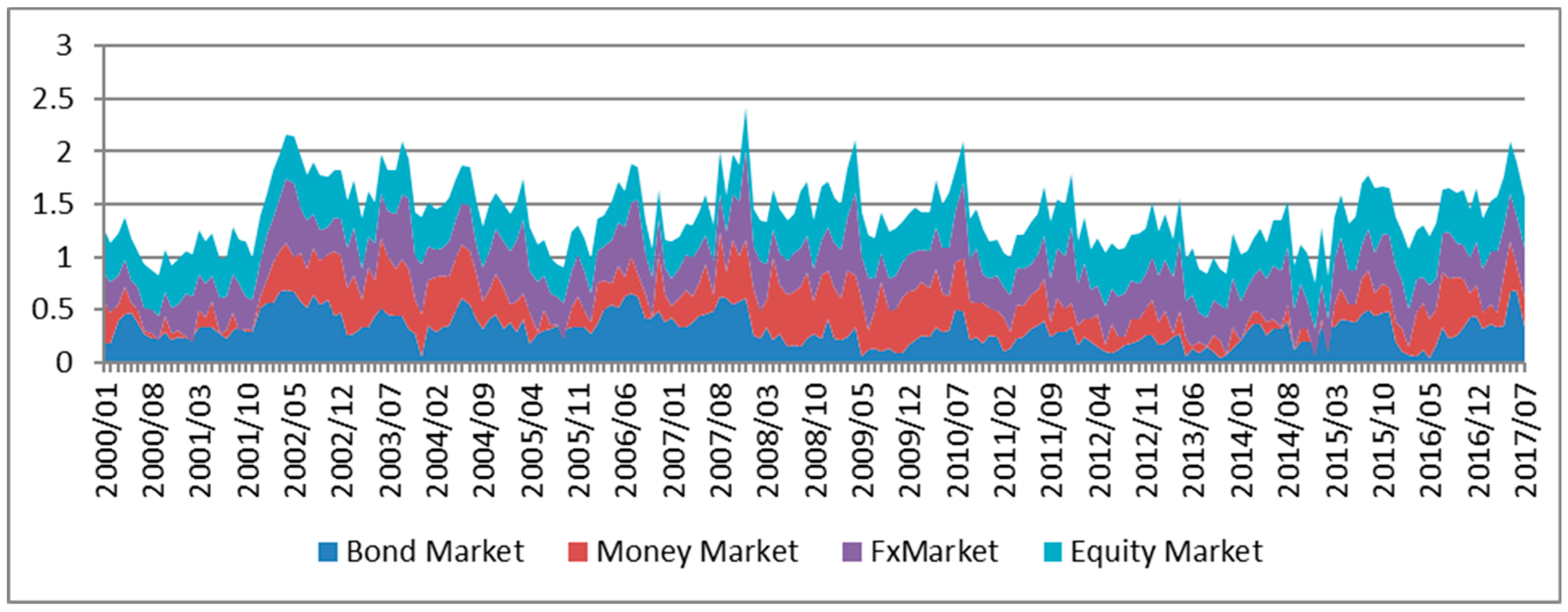
These indicators were grouped into four market segments (Money, bond, equity, and foreign exchange). Each of the raw indicators captures information about the stress level within each market segment. The market segment sub-indices were calculated based on a simple arithmetic average (Figure 1). This implies that each of the raw risk indicators was given equal weight in the sub-index. The indicators for each sub-index captures information about the level of stress in the specific market segment. This also implies that each of the raw liquidity risk indicators was given equal weight in the sub-index.
The sub-index for foreign exchange reached the maximum level during the 2008 global financial crisis.
4.3. Aggregation of Sub-Indices into a Single Composite Index
4.3.1. Variance-Equal Weighting (VEW) Method
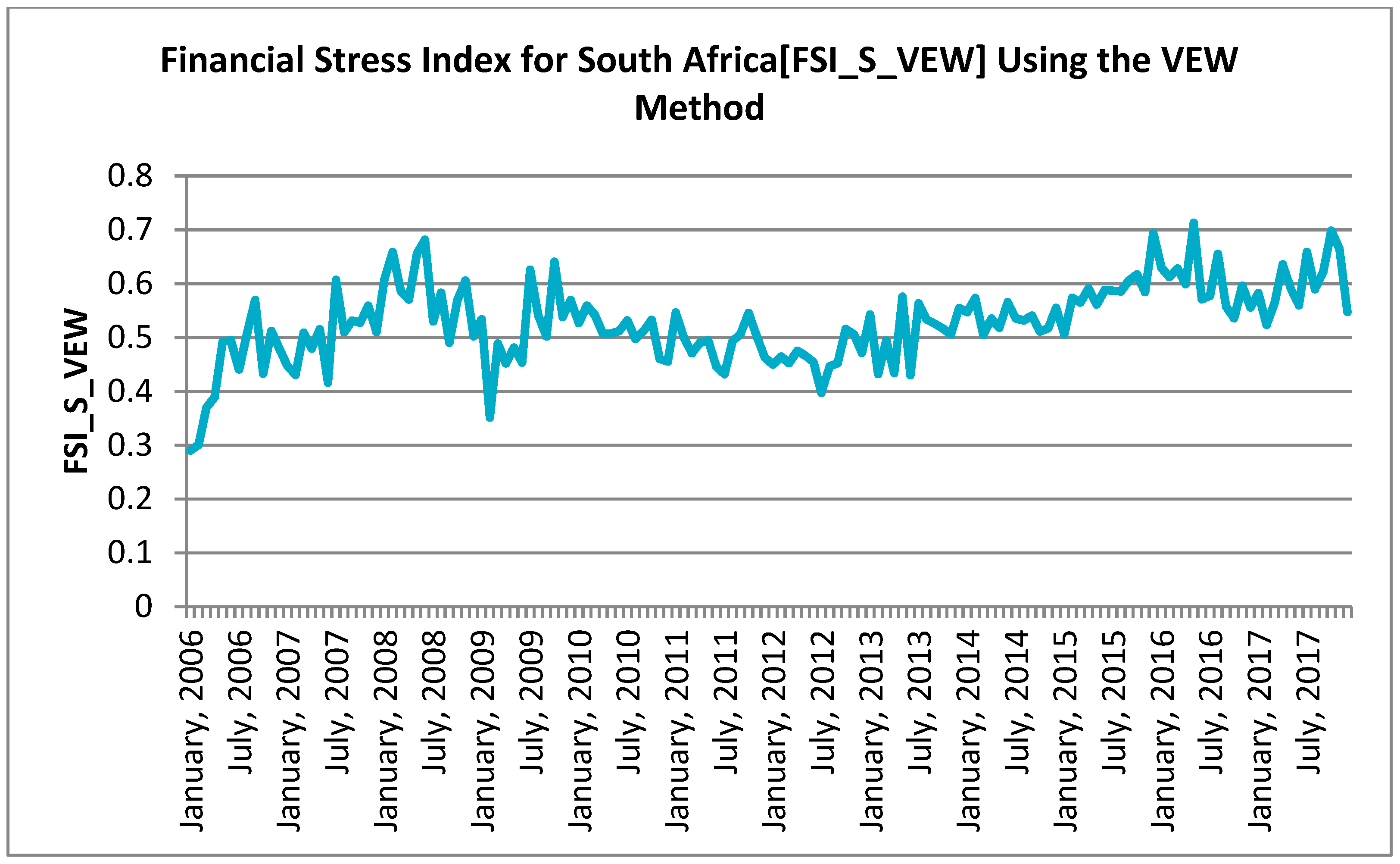
The result of the FSI using the VEW method is presented in Figure 2. This is the most common method used for estimating FSI in previous studies. It is easy to construct and interpret this method compared to other weighing methods. As noted earlier, all the indicators in each market segment were transformed using the empirical standardization method after they are aggregated using the arithmetic mean to derive each market segment sub-indices. The final FSI was then constructed using the arithmetic average of the four sub-indexes. Thus, the index values can be interpreted as the number of standard deviations from the sample mean.
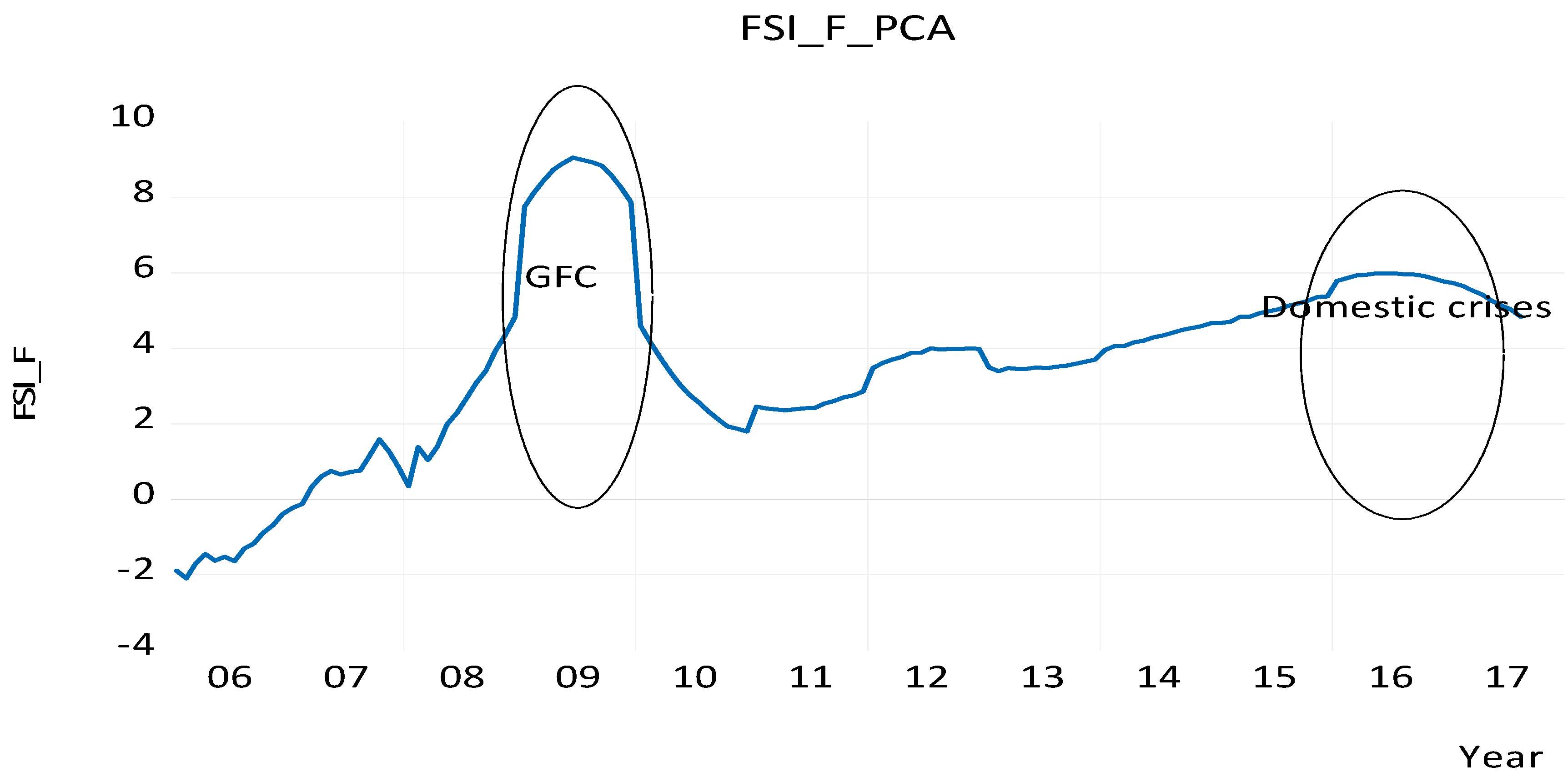
The result as presented in Figure 2 revealed the extreme stress events caused by a global financial crisis and more of domestic crises ranging from a labor crisis, energy crisis and political uncertainty, which started in late 2015 and extended into 2016.
4.3.2. Principal Component Analysis (PCA) Method
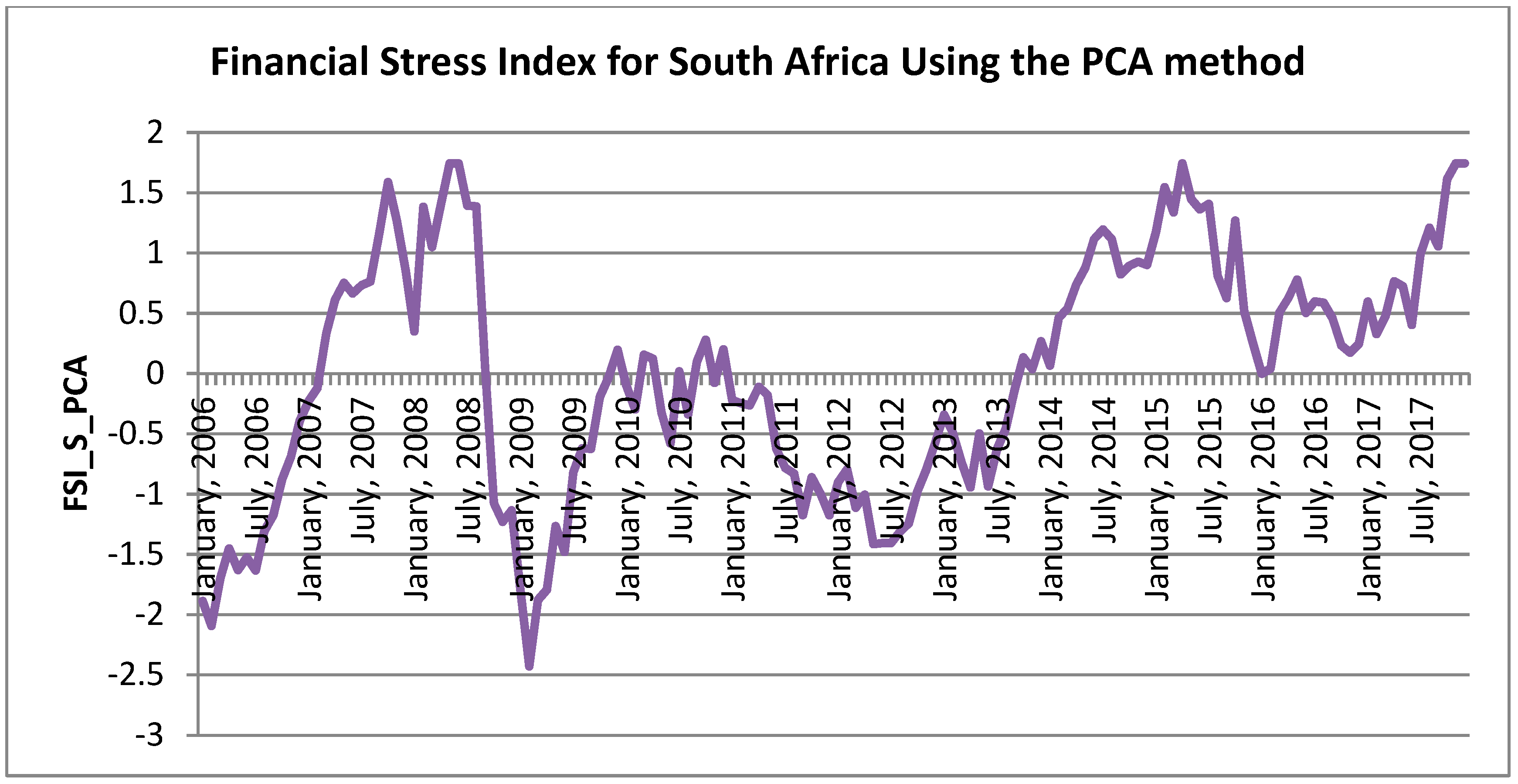
Due to the limitation in the VEW method noted earlier, the FSI was also constructed using the PCA and is presented in Figure 3. Several other studies (Illing and Liu 2006; Hakkio and Keeton 2009; Siņenko et al. 2013; Huotari 2015) have also employed this method for the construction of FSI. For each market category, sub-indexes were then calculated by using the PCA. The PCA takes into account co-movement between stress indicators in each market segment. As noted earlier, the prerequisite for applying PCA is to assess the Kaiser-Meyer-Olkin (KMO) test statistics. In this study, the estimated KMO test statistics of 0.52 was greater than 0.5, this means we could carry out PCA to develop a FSI (See Appendix A). Table 2 presents the eigenvalue and the proportion of the four principal components captured within the market segment sub-indices. However, the first two principal components were used since their eigenvalues were greater than one (1). The Orthogonal rotation is presented in Appendix B. The first principal component (PC) captures the larger proportion of the total variation within the stress indicators. As presented in Table 2, the first PC captures 48 percent of the total variation within the indicators. Logically, the more PC is used for the FSI, the more the total variation that can be captured in the index. Nevertheless, adding more PC to the index also adds noise, which makes it difficult to identify crisis periods. Therefore, the first PC was used to estimate the FSI_S_PCA in line with the study of Levanon et al. (2015).
The principal component (eigenvectors) for the first two components are presented in Table 3. The results show that the coefficient for all the market segment indicators are positive and they represent a one standard deviation change in the respective market segments from the final FSI, since all the indicators are standardized. The coefficients range from a low of 0.43 for the equity market segment to 0.53 for the foreign exchange market segment. The margin is quite small and this implies that all the markets affect the FSI_S_PCA by almost the same proportion, although the foreign exchange market contributes more to the final FSI (Table 3).
4.3.3. Identification of Stress Events
The FSI_S_PCA reflect dynamics in the surge that cause tension within the financial system. As noted earlier, the stress indicators were standardized to values between 0 and 1. This implies that a value of 0, which is the mean of the FSI_S_PCA, would mean that the financial system is experiencing an average risk level. This is therefore adopted as the threshold level above which would suggest extreme conditions or a signal of an impending crisis. The results as presented in Figure 3 revealed previous well-known financial crises. The well-known global financial crisis which began in 2007 as well as the sovereign debt crisis had some impacts on the South African financial system.
The impact of the sub-prime mortgage crisis was then quickly shown to have implications beyond the US. The FSI_S_PCA first signaled an extreme level of stress around August 2007; this was the time when BNP Paribas suspended three investment funds that invested in asset-backed securities linked to the subprime mortgage debts which had become illiquid. Other events happened which led to a rise in the FSI_S_PCA and which reached its maximum level (1.74) around May/June 2008. At this time, global exports were down by 22 percent and Bear Stearns in the US had collapsed (Tooze 2018). By April 2008, the US Treasury and US Federal Reserve Bank had to bail out two financial institutions as the ‘credit freeze’ gripped the country’s financial system. Like a pack of dominoes, most banks with large sub-prime exposures joined the solvency and liquidity scuffle.
As the liquidity situation became more challenging, investors began to withdraw funds from emerging markets in a so-called flight to quality as risk aversion set in. In South Africa, the Johannesburg Securities Exchange all-share index fell from a high of 32,542 on 23 May 2008 to a low of 18,066 on 21 November 2008, but volatility and uncertainty in the market were as worrying as the absolute fall in the index. New listings remained subdued throughout 2009. However, the all-share index then picked up, and it stood at 27,895 at 5 January 2010 (Padayachee 2012). The index increased above the threshold level almost during the entirety of 2008, after which there was a steady decline around February 2009. We also observed a mild increase in stress that was above the threshold of 0 in late 2010 (m4). It later rose in 2014 and reached another peak in 2015 (m4), as well as towards the end of the sample. For the latter part of the FSI_S, domestic factors such as political uncertainty played a role in this trend (Ousting of the former president Jacob Zuma in December 2017).
4.3.4. Forecast Accuracy Evaluation
In this section, the forecasting ability of the FSI_PCA was tested. The Root Mean Square Error (RMSE), Mean Absolute Error (MAE), Theils Inequality Coefficient (TIC), Thiel U2 Coefficient and Symmetric MAPE among others were used and the results are presented in Table 4. For the models forecasting, the in-sample estimation was from 2006m1 to 2008m4, while the out-of-sample forecast was from 2008m5 to 2017m12. All the variables passed the necessary diagnostic test. The forecast was made using the dynamic model.
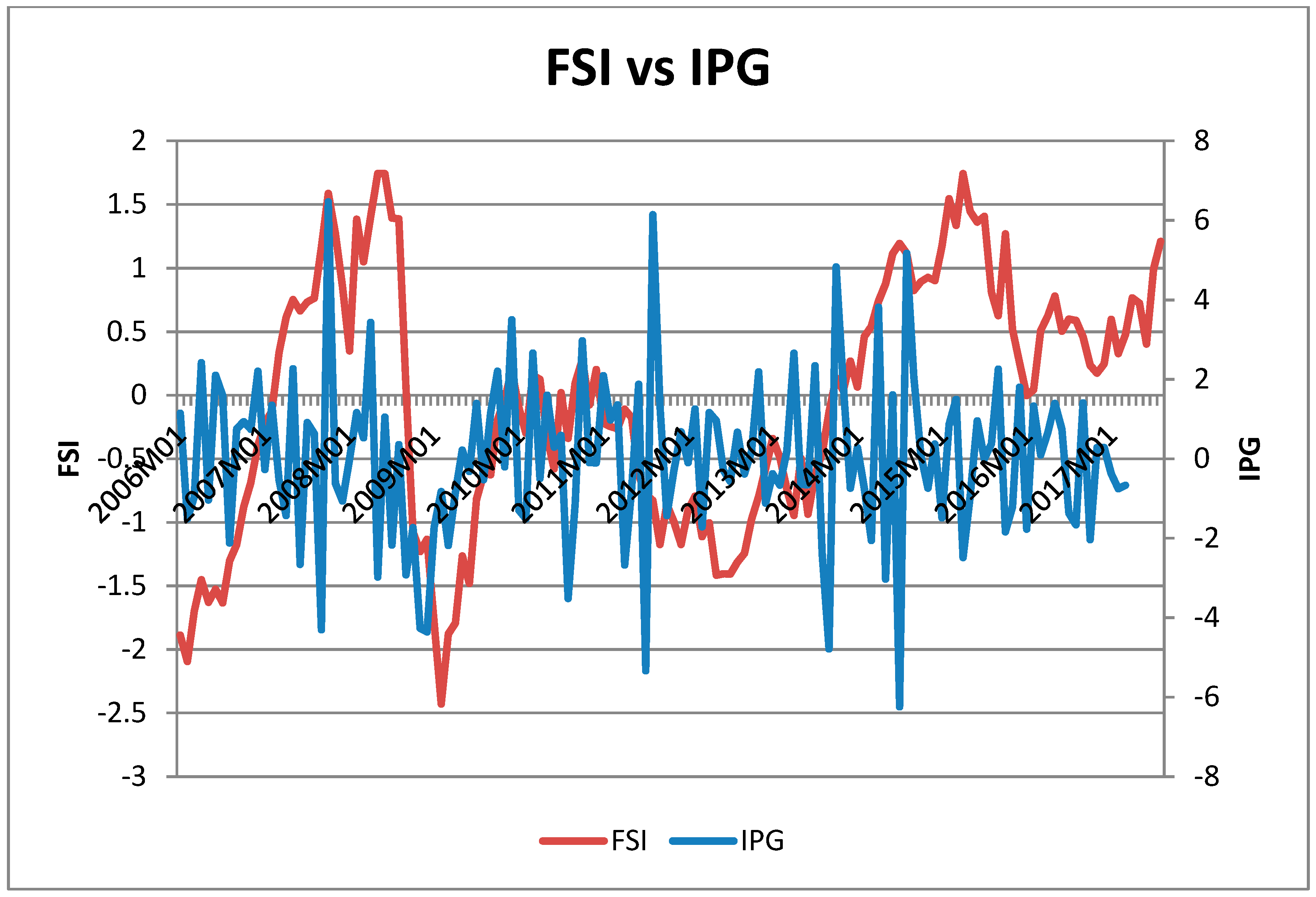
From the results as presented in Table 4, it is clear that the FSI performs very well with regards to its forecasting ability. This is because of the RMSE (5.0166), MAE (4.5585), Theil’s U coefficient (0.8659), U2 (77.4602) and SMAPE (172.5047) of the FSI model. The same goes for the bias, variance and covariance decomposition of the Theil’s coefficient. In Figure 4, the FSI for South Africa using the PCA aggregation method is plotted against the growth rate of industrial production (IPG). It can be seen that periods of high financial stress (2008m5 2015m4) are characterized by low industrial production, though with some time lag as it takes a while for stress to affect industrial output. Also, in the forecasted FSI values plotted in Figure 5, it can be seen that the 2008/09 GFC was picked as well as the domestic crises towards the end of the sample period.
The results as presented in Figure 5 show that both domestic and international shock created uncertainty in the South African financial system. On the international scene, we have the financial crisis while on the domestic scene we have slow growth, a labor crisis and an energy crisis, coupled with political uncertainty.
4.4. FSI and the Real Economy
To avoid spurious regression results, one of the major requirements of time series analysis is to test for stationarity. This study employed the Augmented Dickey-Fuller (ADF) method to test the stationarity of the variables and the result is presented in Table 5. It must be noted that the variables investment (INV) proxied by the gross fixed capital formation and industrial production (IDP) which is the proxy for economic output are in logged form, except for the FSI which is in index form.
The ADF test as presented in Table 5 indicates that the variables FSI, INV and IDP exhibit a unit root problem, which means that they are not stationary at levels. This is because their estimated test statistic values are not more negative than their critical values at the 5 percent level. For stationary of the series to be accomplished, the test for the series was carried out at first difference. The result of the test at first difference shows that all the series are stationary, that is, they are integrated of order one I(1). Having established the order of the integration of the variables of interest, it is important to identify the appropriate lag length for the estimation. To select the lag order of the VAR, the information criteria approach was applied. The sequential modified LR test statistic (each test at 5% level) (LR), Final prediction error (FPE), Akaike information criterion (AIC), Schwarz information criterion (SIC) and Hannan-Quinn information criterion (HQ) lag lengths information criterion was employed to determine the lag length, and we chose 3 lag length for the estimated VAR (See Appendix C).
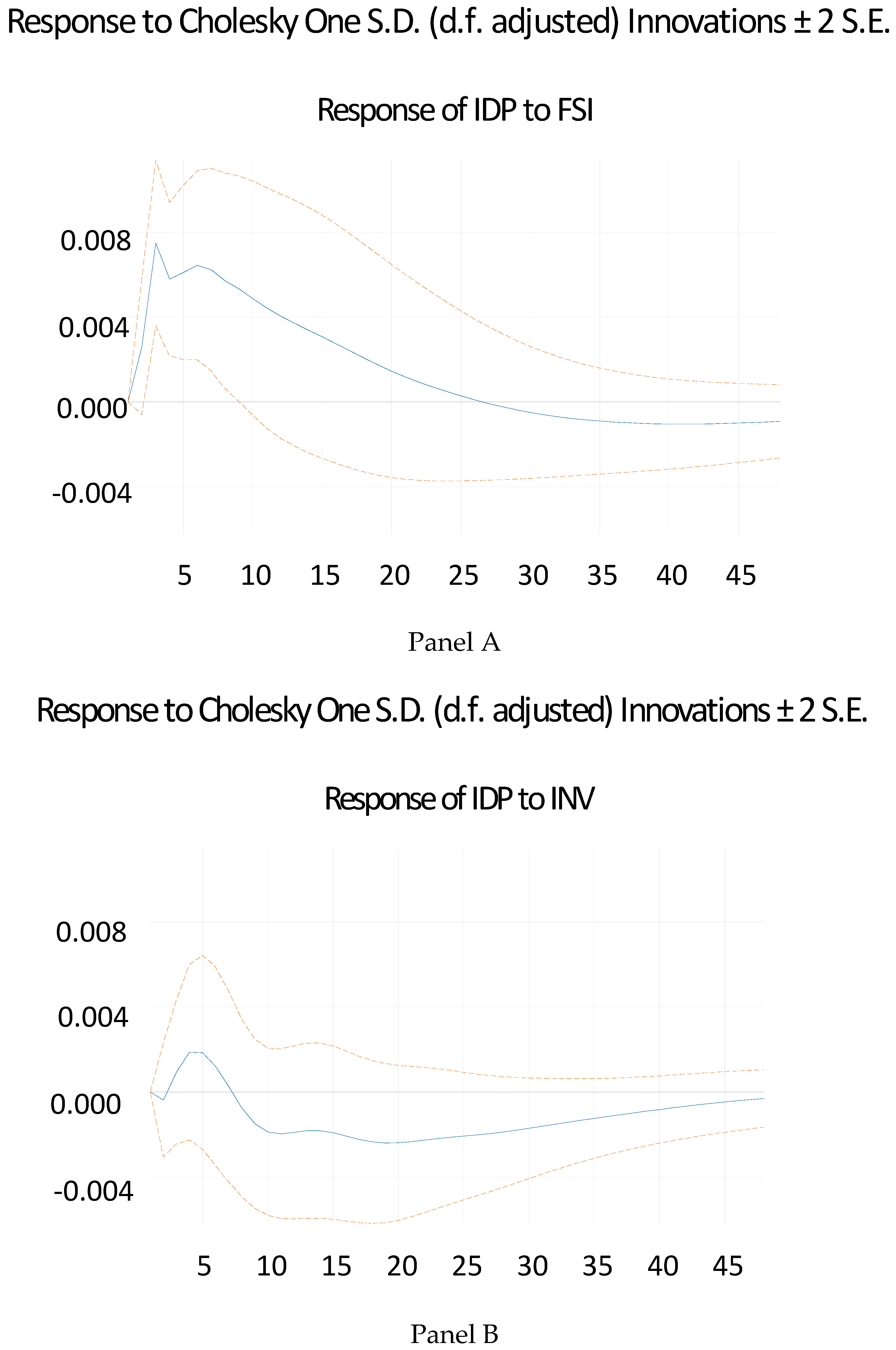
Furthermore, the study employed the Cholesky impulse response to the impact of financial stress on investment and output proxied by industrial production. It must be noted that the impulse response function indicates the effect of one standard deviation shocks to one of the innovations on the adjustment path of the variables. The impulse response function reflecting the direction and magnitude of the linkages between the FSI based on the principal components as the aggregation method and the real economy is presented in Figure 6A,B.
The result of the IRF as shown in panel a of Figure 6 indicates that with a one-unit shock in FSI, IDP first responds positively and thereafter began to fall after 3 months until it becomes negative. It must be noted that the point where the IRF becomes negative corresponds to the peak of the FSI.
This corresponds to the study of Stolbov and Shchepeleva (2016). During this period, domestic output fell significantly. Specifically, the manufacturing sector contracted by 20 percent during the period of the crisis, with the majority of job losses coming from the sector (Coleman 2009). The result, therefore, indicates that though the immediate impact of financial stress is not pronounced, it does have a negative future impact of output. This is similar to the study of Sahoo (2020) in the case of India. In this study, it was revealed that financial stress does harm growth but with a certain time lag. Furthermore, the results indicated in panel b of Figure 6 show that investment falls during financial stress periods but only after about 7 months. The highest decline in investment due to financial shock seems to occur approximately a year into the shock. The result is similar to the study of Malega and Horváth (2017). This, therefore, implies that there should be a concerted effort to stimulate investment and domestic production by relevant stakeholders to mitigate the impact of financial stress.
5. Conclusions
This study contributes to the existing body of knowledge by constructing a financial stress index for South Africa, as well as by examining its effects on the real economy. The construction of the financial stress index is important, as it combines the underlying factors in the various segments of the economy at any given point in time. The FSI is also useful and appropriate as the dependent variable in an early signal warning model. It can further be used to gauge the effectiveness of government measures to mitigate the impact of financial stress. A Financial stress index was constructed for the South African financial system using monthly series for 13 indicators, which were grouped into four (4) sub-indices: the money market, bond market, foreign exchange market, and the real estate market and equity market. The VEW and PCA methods were used in the aggregation of the indicators.
The result indicates that extreme values of FSIs are associated with well-known financial stress cases. It must be noted that the FSI constructed based on PCA provides importance to indicators with higher volatility. The result shows that both the domestic and international shocks created uncertainty in the South African financial system. On the international scene, we have the financial crisis while on the domestic scene we have slow growth, a labor crisis and political uncertainly. Furthermore, it was revealed that financial stress also affected domestic production and investment negatively, though not immediately. A concerted effort to stimulate investment and domestic production by relevant stakeholders is necessary to mitigate the impact of financial stress. This will go a long way to alleviating the impact of the financial stress on industrial production, employment and the economy at large.
Supplementary Materials
The following are available online at https://0-www-mdpi-com.brum.beds.ac.uk/2227-7099/8/4/110/s1, Data used in the research.
Author Contributions
Conceptualization, methodology, software, formal analysis, writing—original draft preparation, writing—review and editing, K.D.I.; writing—review and editing, supervision, D.D.T. All authors have read and agreed to the published version of the manuscript.
Funding
This research received no external funding.
Conflicts of Interest
The authors declare no conflict of interest.
Appendix A. Kaiser-Meyer-Olkin Measure of Sampling Adequacy
| Variable | Kmo |
| Money market | 0.5025 |
| Bond market | 0.5482 |
| Equity market | 0.5448 |
| Foreign exchange market | 0.4895 |
| Overall | 0.5219 |
Appendix B. Orthogonal Rotation
| Principal components/correlation Number of obs | 144 | |||
| Number of comp. | 2 | |||
| Trace | 4 | |||
| Rotation: orthogonal varimax (Kaiser off) Rho | 0.7862 | |||
| Component | Variance | Difference | Proportion | Cumulative |
| Comp1 | 1.60838 | 0.071834 | 0.4021 | 0.4021 |
| Comp2 | 1.53654 | 0.3841 | 0.7862 | |
| Rotated components | ||||
| Variable | Comp1 | Comp2 | Unexplained | |
| Money market | 0.7193 | −0.0454 | 0.1868 | |
| Bond market | 0.0857 | 0.6767 | 0.2452 | |
| Equity market | 0.6853 | 0.043 | 0.2218 | |
| Foreign exchange market | −0.0747 | 0.7336 | 0.2013 | |
| Component rotation matrix | ||||
| Comp1 | Comp2 | |||
| Comp1 | 0.7435 | 0.6688 | ||
| Comp2 | −0.6688 | 0.7435 | ||
Appendix C. VAR Lag Order Selection Criteria

| VAR Lag Order Selection Criteria | ||||||
| Endogenous variables: IDP FSI INV | ||||||
| Exogenous variables: C | ||||||
| Date: 07/14/20 Time: 15:35 | ||||||
| Sample: 2006M01 2017M12 | ||||||
| Included observations: 139 | ||||||
| Lag | LogL | LR | FPE | AIC | SC | HQ |
| 0 | 231.5556 | NA | 7.49 × 10⁻⁹ | −3.288570 | −3.225236 | −3.262832 |
| 1 | 734.8705 | 977.6620 | 6.10 × 10⁻⁹ | −10.40101 | −10.14768 | −10.29807 |
| 2 | 807.1346 | 137.2499 | 2.46 × 10⁻⁹ | −11.31129 | −10.86795 | −11.13113 |
| 3 | 850.8368 | 81.11628 * | 1.49 × 10⁻⁹ * | −11.81060 * | −11.17726 * | −11.55323 * |
| 4 | 855.5381 | 8.523214 | 1.59 × 10⁻⁹ | −11.74875 | −10.92541 | −11.41417 |
| 5 | 863.6863 | 14.42053 | 1.61 × 10⁻⁹ | −11.73649 | −10.72315 | −11.32470 |
* indicates lag order selected by the criterion; LR: sequential modified LR test statistic (each test at 5% level); FPE: Final prediction error; AIC: Akaike information criterion; SC: Schwarz information criterion; HQ: Hannan-Quinn information criterion.
References
- Aklan, Nejla, Mehmet Çinar, and Akay Hülya. 2015. Financial Stress and Economic Activity Relationship in Turkey: Post-2002 Period. Yonetim Ve Ekonomi 22: 567–80. [Google Scholar]
- Alberola, Enrique, Carlos Trucharte, and Juan Luis Vega. 2011. Central Banks And Macroprudential Policy—Some Reflections from the Spanish Experience. Documentos Ocasionales-Banco de España 5: 5–26. [Google Scholar] [CrossRef] [Green Version]
- Balakrishnan, Ravi, Stephan Danninger, Selim Elekdag, and Irina Tytell. 2011. The Transmission Of Financial Stress From Advanced To Emerging Economies. Emerging Markets Finance And Trade 47: 40–68. [Google Scholar]
- Brockmeijer, Jan, Moretti Marina, Osinski Jacek, Blancher Nicholas, Gobat Jeanne, Jassaud Nadege, Lim Cheng Hoon, Loukoianova Elena, Mitra Srobona, Nier Erlend, and et al. 2011. Macro Prudential Policy: An Organizing Framework. IMF, March 14. [Google Scholar]
- Cambón, Mª Isabel, and Leticia Estévez. 2016. A Spanish Financial Market Stress Index (Fmsi). The Spanish Review of Financial Economics 14: 23–41. [Google Scholar]
- Cardarelli, Roberto, Selim Elekdag, and Subir Lall. 2011. Financial Stress And Economic Contractions. Journal of Financial Stability 7: 78–97. [Google Scholar] [CrossRef]
- Central Bank of the Republic of Turkey. 2009. Financial Stability Report; Central Bank of the Republic of Turkey: Novermber 2006. vol. 9. Available online: https://www.tcmb.gov.tr/wps/wcm/connect/726264e3-e640-47f5-9aac-e4c237923b23/fulltext9.pdf?MOD=AJPERES&CACHEID=ROOTWORKSPACE-726264e3-e640-47f5-9aac-e4c237923b23-m3fw7hd (accessed on 10 January 2017).
- Cevik, Emrah Ismail, Sel Dibooglu, and Ali M. Kutan. 2013. Measuring Financial Stress in Transition Economies. Journal of Financial Stability 9: 597–611. [Google Scholar] [CrossRef]
- Coleman, E. 2009. South Africa’s Response to the Global Economic Crisis: Ministerial Briefing. Available online: https://pmg.org.za/committee-meeting/10717/ (accessed on 9 November 2020).
- D’Antonio, Peter. 2008. A View of the U.S. Subprime Crisis. Ema Special Report. Edited by Robert Diclemente and Kermit Schoenholtz. New York: Citigroup Global Markets Inc., pp. 26–28. [Google Scholar]
- Davig, Troy, and Craig Hakkio. 2010. What Is the Effect Of Financial Stress on Economic Activity. Economic Review. Kansas City: Federal Reserve Bank of Kansas City, vol. 95, pp. 35–62. [Google Scholar]
- De Bandt, Olivier, and Philipp Hartmann. 2000. Systemic Risk: A Survey. CEPR Discussion Papers. p. 2634. Available online: https://papers.ssrn.com/sol3/papers.cfm?abstract_id=258430 (accessed on 10 January 2016).
- Ekinci, Aykut. 2013. Financial Stress Index For Turkey. Doğuş Üniversitesi Dergisi 14: 213–29. [Google Scholar] [CrossRef]
- Hakkio, Craig S., and William R. Keeton. 2009. Financial Stress: What Is It, How can It Be Measured, and Why Does It Matter? Economic Review 94: 5–50. [Google Scholar]
- Havránek, Tomáš, Roman Horváth, and Jakub Matějů. 2012. Monetary Transmission and the Financial Sector in the Czech Republic. Economic Change and Restructuring 45: 135–55. [Google Scholar] [CrossRef]
- Holló, Daniel, Manfred Kremer, and Marco Lo Duca. 2012. CISS—A Composite Indicator of Systemic Stress in The Financial System. Available online: https://papers.ssrn.com/sol3/papers.cfm?abstract_id=2018792 (accessed on 10 January 2017).
- Hooper, Peter, Slok Torsten, and Dobridge Christine. 2010. Improving Financial Conditions Bode Well For Growth. Global Economic Perspectives. Frankfurt: Deutsche Bank. [Google Scholar]
- Hotelling, Harold. 1933. Analysis of a Complex of Statistical Variables into Principal Components. Journal of Educational Psychology 24: 417. [Google Scholar] [CrossRef]
- Huotari, Jarkko. 2015. Measuring Financial Stress—A Country Specific Stress Index for Finland. Available online: https://papers.ssrn.com/sol3/papers.cfm?abstract_id=2584378 (accessed on 10 January 2017).
- Iachini, Eleonora, and Stefano Nobili. 2016. Systemic Liquidity Risk And Portfolio Theory: An Application To The Italian Financial Markets. The Spanish Review of Financial Economics 14: 5–14. [Google Scholar] [CrossRef]
- Ilesanmi, Kehinde Damilola, and Devi Datt Tewari. 2019a. Developing a Financial Stress Index for the Nigerian Financial System. African Journal of Business And Economic Research 14: 135–57. [Google Scholar] [CrossRef]
- Ilesanmi, Kehinde Damilola, and Devi Datt Tewari. 2019b. Management of shadow banks for economic and financial stability in South Africa. Cogent Economics & Finance 7: 1–13. [Google Scholar] [CrossRef] [Green Version]
- Illing, Mark, and Ying Liu. 2006. Measuring Financial Stress in a Developed Country: An Application to Canada. Journal of Financial Stability 2: 243–65. [Google Scholar] [CrossRef]
- Islami, Mevlud, and Jeong-Ryeol Kurz-Kim. 2014. A Single Composite Financial Stress Indicator and Its Real Impact in the Euro Area. International Journal of Finance & Economics 19: 204–11. [Google Scholar]
- Kabundi, Alain, and Asithandile Mbelu. 2020. Estimating A Time-Varying Financial Conditions Index for South Africa. Empirical Economics, 1–28. [Google Scholar] [CrossRef]
- Kama, Ukpai, M. Adigun, and Olubukola Adegbe. 2013. Issues and Challenges for the Design and Implementation of Macro-Prudential Policy in Nigeria. Occasional Paper No. 46. Abuja: Central Bank of Nigeria. [Google Scholar]
- Kočišová, Kristína, and Daniel Stavarek. 2015. Banking Stability Index: New Eu Countries after Ten Years of Membership (No. 0024). Available online: http://www.iivopf.cz/images/Working_papers/WPIEBRS_24_Kocisova_Stavarek.pdf (accessed on 10 January 2018).
- Kondratovs, Kirils. 2014. Modelling Financial Stability Index for Latvian Financial System. Regional Formation and Development Studies 3: 118–30. [Google Scholar]
- Levanon, Gad, Jean-Claude Manini, Ataman Ozyildirim, Brian Schaitkin, and Jennelyn Tanchua. 2015. Using Financial Indicators to Predict Turning Points in the Business Cycle: The Case of the Leading Economic Index for the United States. International Journal of Forecasting 31: 426–45. [Google Scholar] [CrossRef]
- Liao, Shuyu, Elvira Sojli, and Wing Wah Tham. 2015. Managing Systemic Risk in The Netherlands. International Review of Economics and Finance 40: 231–45. [Google Scholar] [CrossRef]
- Lütkepohl, H. 2006. Structural vector autoregressive analysis for cointegrated variables. Allgemeines Statistisches Archiv 90: 75–88. [Google Scholar]
- Malega, Ján, and Roman Horváth. 2017. Financial Stress in the Czech Republic: Measurement and Effects on the Real Economy. Prague Economic Papers 26: 257–68. [Google Scholar] [CrossRef] [Green Version]
- Manizha, Sharifova. 2014. Essays on Measuring Systemic Risk. Santa Cruz: University of Califonia Santa Cruz, Available online: http://0-Scholar-Google-Com.brum.beds.ac.uk/Scholar?Hl=En&Btng=Search&Q=Intitle:Electronic+Theses+And+Dissertations+Uc+Santa+Cruz#0 (accessed on 10 January 2017).
- Mundra, Sruti, and Motilal Bicchal. 2020. Evaluating Financial Stress Indicators: Evidence From Indian Data. Journal of Financial Economic Policy. [Google Scholar] [CrossRef]
- Nelson, William R., and Roberto Perli. 2007. Selected Indicators of Financial Stability. Risk Measurement And Systemic Risk 4: 343–72. [Google Scholar]
- Oet, Mikhail V., Ryan Eiben, Timothy Bianco, Dieter Gramlich, and Stephen J. Ong. 2011. The Financial Stress Index: Identification of Systemic Risk Conditions. Working Papers of the Federal Reserve Bank of Cleveland. pp. 11–30. Available online: https://papers.ssrn.com/sol3/papers.cfm?abstract_id=1917727 (accessed on 10 January 2020).
- Padayachee, Vishnu. 2012. Global economic recession: Effects an implications for South Africa at a time of political challenges. Paper presented at the 20th anniversary LSE Department of International Development Conference, September 2011, viewed 23 May 2013. Available online: http://www.lse.ac.uk/internationalDevelopment/20thAnniversaryConference/ImpactoftheGlobalFC.pdf (accessed on 10 November 2020).
- Park, Cyn-Young, and Rogelio V. Mercado Jr. 2014. Determinants of Financial Stress in Emerging Market Economies. Journal of Banking & Finance 45: 199–224. [Google Scholar]
- Pearson, Karl. 1901. Principal Components Analysis. The London, Edinburgh, and Dublin Philosophical Magazine and Journal of Science 6: 559. [Google Scholar] [CrossRef] [Green Version]
- Rosenberg, Michael. 2009. Financial Conditions Watch. Bloomberg, December 3. [Google Scholar]
- Sahoo, Jayantee. 2020. Financial Stress Index, Growth And Price Stability in India: Some Recent Evidence. Transnational Corporations Review, 1–15. [Google Scholar] [CrossRef]
- South African Reserve Bank. 2015. Financial Stability Review, 2nd ed. Pretoria: SARB. [Google Scholar]
- Siņenko, Nadežda, Deniss Titarenko, and Mikus Āriņš. 2013. The Latvian Financial Stress Index As an Important Element of the Financial System Stability Monitoring Framework. Baltic Journal of Economics 13: 87–113. [Google Scholar] [CrossRef]
- Stolbov, Mikhail, and Maria Shchepeleva. 2016. Financial Stress in Emerging Markets: Patterns, Real Effects, and Cross Country Spillovers. Review of Development Finance 6: 71–81. [Google Scholar] [CrossRef] [Green Version]
- Tooze, Adam. 2018. The Forgotten History of the Financial Crisis: What the World Should Have Learned in 2008. Available online: https://www.foreignaffairs.com/articles/world/2018-08-13/forgotten-history-financial-crisis (accessed on 10 March 2019).
- Yellen, Janet L. 2010. Macroprudential Supervision and Monetary Policy in the Post-Crisis World. Business Economics 46: 3–12. [Google Scholar] [CrossRef] [Green Version]
| 1 | |
| 2 | Note: FSI stands for South African financial stress index using the PCA method; IDP for industrial production which was proxied by manufacturing output; INV for investment rate which is proxied by gross fixed capital formation. |
Figure 1.
Sub-indices for the four market indices.

Figure 2.
Financial Stress Index for South Africa Using the VEW Method.

Figure 3.
Financial Stress Index for South Africa Using the PCA Method.

Figure 4.
FSI for South Africa using the PCA and the growth rate of industrial production (IPG).

Figure 5.
FSI forecast (FSI_F) for South Africa using the PCA.

Figure 6.
(A,B) Impulse Response between Financial stress index and the real economy2.
Figure 6.
(A,B) Impulse Response between Financial stress index and the real economy2.

Table 1.
Descriptive Statistics for the South Africa Financial Sector
| Variable N | Nos of Observation | Mean | Std. Dev. | Min | Max |
|---|---|---|---|---|---|
| VIR | 144 | 0.665735 | 0.143452 | 0 | 1 |
| ILS | 144 | 0.180793 | 0.137266 | 0 | 1 |
| ICB | 144 | 0.738199 | 0.101617 | 0 | 1 |
| VBY | 144 | 0.369467 | 0.129358 | 0 | 1 |
| SBS | 144 | 0.583882 | 0.210692 | 0 | 1 |
| VUZ | 144 | 0.44274 | 0.160191 | 0 | 1 |
| VGZ | 144 | 0.530947 | 0.15324 | 0 | 1 |
| VEZ | 144 | 0.510652 | 0.159521 | 0 | 1 |
| MUZ | 144 | 0.493765 | 0.293897 | 0 | 1 |
| MGZ | 144 | 0.577762 | 0.263284 | 0 | 1 |
| MEZ | 144 | 0.591845 | 0.240057 | 0 | 1 |
| VAI | 144 | 0.592538 | 0.157898 | 0 | 1 |
| MAI | 144 | 0.582082 | 0.239655 | 0 | 1 |
| **MMS | 144 | −4.04 × 10⁻⁹ | 1.000002 | −7.26451 | 2.576354 |
| **BMS | 144 | −4.90 × 10⁻⁹ | 1 | −2.77126 | 1.975004 |
| **FXM | 144 | −1.55 × 10⁻⁹ | 1.000002 | −2.46544 | 1.700248 |
| **EMS | 144 | 2.06 × 10⁻⁹ | 1 | −2.42883 | 1.743836 |
| FSI_S_KD | 144 | −2.99 × 10⁻⁹ | 1.000003 | −2.42884 | 1.743845 |
** MMS is the money market sub-index; BMS is the bond market sub-index; FXM is the foreign exchange market sub-index and EMS is the equity market sub-index.
Table 2.
Eigenvalue and Proportion of each Component in the PCA.
| Components | Eigenvalue | Proportion | Cumulative |
|---|---|---|---|
| Component 1 | 1.91296 | 0.4782 | 0.4782 |
| Component 2 | 1.23195 | 0.3080 | 0.7862 |
| Component 3 | 0.500228 | 0.1251 | 0.9113 |
| Component 4 | 0.354856 | 0.0887 | 1.0000 |
Source: Estimation.
Table 3.
Principal components (eigenvectors) for the first two component.
| Market Segment | Component 1 | Component 2 | Unexplained |
|---|---|---|---|
| Money market | 0.5044 | −0.5148 | 0.1868 |
| Bond market | 0.5163 | 0.4458 | 0.2452 |
| Equity market | 0.4350 | −0.4264 | 0.2218 |
| Foreign exchange market | 0.5383 | 0.5953 | 0.2013 |
Source: Estimation.
Table 4.
Forecast model evaluation.
| RMSE | MAE | MAPE | Theil | Theil U2 | Bias | Variance | Covariance | SMAPE | |
|---|---|---|---|---|---|---|---|---|---|
| FSI_F_PCA | 5.0166 | 4.5585 | 4161.045 | 0.8659 | 77.4602 | 0.8257 | 0.0301 | 0.1442 | 172.5047 |
RMSE: Root Mean Square Error; MAE: Mean Absolute Error; MAPE: Mean Absolute Percentage Error; Theil: Theil inequality coefficient; Theil U2 Coefficient; Bias, variance and covariance are the decomposed proportions of the Theil’s Inequality coefficient.
Table 5.
ADF Stationarity Test Result.
| Variables | T Statistic | Critical Value (5%) | Lag Length (Automatic—Based on SIC) | Integrated Order | Restriction |
|---|---|---|---|---|---|
| FSI | −2.388850 | −2.881685 | 0 | I(0) | Constant |
| D(FSI) | −11.73655 | −2.881830 | 0 | I(1) * | Constant |
| INV | −2.092949 | −2.882748 | 0 | I(0) | Constant |
| D(INV) | −3.717822 | −2.883930 | 13 | I(1) * | Constant |
| IDP | −2.104219 | −2.881830 | 1 | I(0) | Constant |
| D(IDP) | −15.46115 | −2.881830 | 0 | I(1) * | Constant |
Source: Estimation * means significant at a 5 percent level.
Publisher’s Note: MDPI stays neutral with regard to jurisdictional claims in published maps and institutional affiliations. |
© 2020 by the authors. Licensee MDPI, Basel, Switzerland. This article is an open access article distributed under the terms and conditions of the Creative Commons Attribution (CC BY) license (http://creativecommons.org/licenses/by/4.0/).
Share and Cite
MDPI and ACS Style
Ilesanmi, K.D.; Tewari, D.D. Financial Stress Index and Economic Activity in South Africa: New Evidence. Economies 2020, 8, 110. https://0-doi-org.brum.beds.ac.uk/10.3390/economies8040110
AMA Style
Ilesanmi KD, Tewari DD. Financial Stress Index and Economic Activity in South Africa: New Evidence. Economies. 2020; 8(4):110. https://0-doi-org.brum.beds.ac.uk/10.3390/economies8040110
Chicago/Turabian StyleIlesanmi, Kehinde Damilola, and Devi Datt Tewari. 2020. "Financial Stress Index and Economic Activity in South Africa: New Evidence" Economies 8, no. 4: 110. https://0-doi-org.brum.beds.ac.uk/10.3390/economies8040110
Note that from the first issue of 2016, this journal uses article numbers instead of page numbers. See further details here.