Decomposing Inequality in Household Consumption Expenditure in Malaysia


School of Mathematical Sciences, Universiti Sains Malaysia, USM Penang 11800, Malaysia
*
Author to whom correspondence should be addressed.
Economies 2020, 8(4), 83; https://0-doi-org.brum.beds.ac.uk/10.3390/economies8040083
Submission received: 5 August 2020
/
Revised: 18 September 2020
/
Accepted: 30 September 2020
/
Published: 14 October 2020
Abstract
:This study aims to examine the sources and determinants of consumption expenditure inequality in Malaysia as well as to quantify their proportional contributions to the total explained inequality using the Household Expenditure Survey (HES) data for the year 2014 collected from the Malaysian Department of Statistics (DOSM). The study applies Field’s regression-based decomposition method to the log-linear regression model of per capita monthly consumption expenditure. It is found that the model explains about 55.2% of the variability in the logged monthly consumption expenditure per capita. The findings suggest that the size of households, education of household heads, and regional variations are the major contributing factors to consumption expenditure inequality in Malaysia, with household size being among the highest. Other household head characteristics, including ethnicity, strata, and citizenship, have small contributions to the total explained inequality. However, sex and age of household heads contributed negatively to inequality and have inequality decreasing effects, with a negative impact on inequality. A large percentage of unexplained inequality is not captured by these factors, which may be attributed to either unobserved household attributes or residuals. The results are important for policy implications and should be taken into account in formulating future policies, especially those aiming to reduce inequality among the population and thus improving living standards and well-being.
1. Introduction
Economic theory defines economic inequality as the unequal distribution of individuals or households’ income or consumption within a certain country and across regions or countries. Inequality, its levels, and its decomposition have received much debate worldwide where the inequality is expressed in terms of income or its components such as wages. However, economists frequently refer to the consumption expenditure to study inequality in living standards rather than income (Meyer and Sullivan 2003; Goodman and Oldfield 2004; Attanasio and Pistaferri 2016). Friedman (1957) exhibited that consumption expenditure is a better proxy measure of households’ welfare and may accurately measure living standards rather than income. Furthermore, Meyer and Sullivan (2006) postulated that the consumption expenditure data provide a better measure of perpetual household income and the poor household’s welfare.
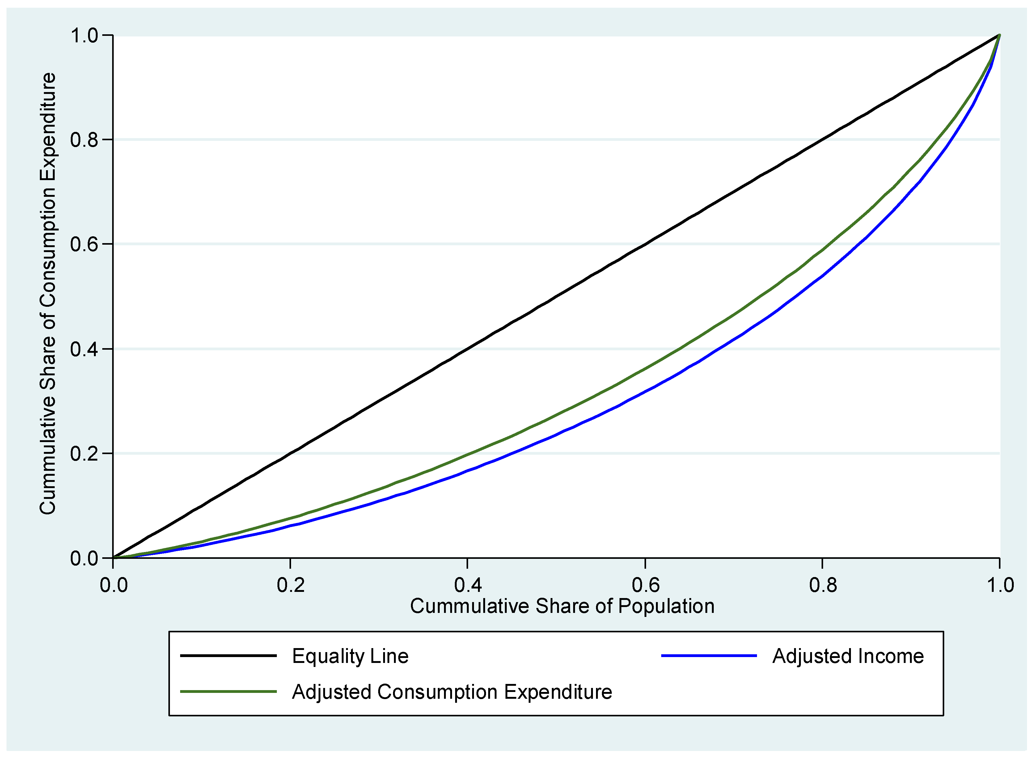
Over the past years, official statistics indicate that Malaysia exhibited a decreasing trend in income inequality, which has been declined from 0.461 in 2002 to 0.399 in 2016 (Safari and Masseran 2019; Malaysian Department of Statistics (DOSM) 2016b). The department of statistics in Malaysia measures income inequality using the Gini coefficient from the Household Income Survey (HIS). However, this may not reflect the actual picture of how the living standard of households is distributed. The HIS may suffer from under-sampling problems that might lead to underestimations of inequality measures, especially in the upper tail of income distribution (Man and NG 2018). Alternatively, the distribution of consumption expenditure plays a vital role in the Malaysian economy in which economic policies are motivated to distribute fundamental resources to all residents equally, which might provide a comprehensive measure of inequality among households rather than income. Malaysian official statistics exhibited an increase in the average monthly household consumption expenditure in Malaysian Ringgits (RM) 4033 in 2016, compared to RM 3578 in 2014, as stated in the Household Expenditure Survey (HES) 2016 report (Malaysian Department of Statistics (DOSM) 2016a). The Gini index based on consumption expenditure data is estimated as 0.330 in 20141, which is comparatively less than the Gini index obtained from income data. Figure 1 shows the Lorenz curves of adjusted income and adjusted consumption expenditure per capita for the year 2014, which confirms that income inequality is higher than consumption expenditure inequality in Malaysia. Considering the prevalence of inequality in Malaysia, there is a need to understand and examine the influential factors of consumption expenditure inequality. To this end, the scopes of the available evidence in Malaysia are mainly descriptive and mostly relied on income rather than consumption expenditure. Besides, the proportionate effects and contributions of various households’ characteristics on the consumption expenditure inequality have not yet been examined in Malaysia, especially those applied the regression-based decomposition method, to the best of the authors’ knowledge. Therefore, it is not obvious to what extent the characteristics of household heads could explain consumption expenditure inequality in Malaysia.
Therefore, this study aims to investigate the determinants or sources of inequality in the distribution of household consumption expenditure in Malaysia. It decomposes the total explained inequality in consumption expenditure components based on Fields’ (2003) decomposition method. Using this approach allows for quantifying the contribution for each factor to consumption expenditure inequality. This study utilizes data of the Household Expenditure Survey (HES) for the year 2014 collected by the DOSM. This study contributes to the existing empirical literature on household consumption expenditure inequality decomposition in various ways. First, it is one of the few studies to examine the contributing factors of consumption expenditure inequality in Malaysia using Fields’ regression-based decomposition approach. Second, the most important findings to emerge from this study reveal that the household size and education of household heads are found to be the major determinants of consumption expenditure inequality in Malaysia. Besides these factors, the state is another important influential factor to the total explained inequality in Malaysia. Meanwhile, strata, ethnicity, and citizenship of household heads make little contributions to the total explained inequality. However, the age and gender of household heads had inequality decreasing effects. Finally, the current study deepens the existing literature in terms of providing complementary and essential information on understanding the models of welfare and household consumption expenditures in Malaysia, which might provide useful and important information on the consumption expenditure distribution dynamics and thus helping decision-making in formulating proper policies aimed to reduce inequality at both household and national levels.
The rest of this study is organized as follows. Section 2 provides a literature review on methodological and empirical related studies. Section 3 describes the data, methodology, and variables used in this paper. Section 4 presents the results and discussions of the empirical findings. The last section concludes the study.
2. Literature Review
The results of various researches across different countries indicate that inequality, either in income or consumption expenditure, is a prevalent phenomenon, which would portend political and social stability (Pieters 2011). For instance, Meyer and Sullivan (2017) illustrated expenditure and income inequalities in the U.S. over the 1963–2014 period. They measured inequality using a 90/10 ratio and showed that the overall income inequality increased over this period, but a small increase was accounted for in overall expenditure inequality. According to Cingano (2014), the gap between rich and poor in most Organisation for Economic Co-operation and Development (OECD) populations exhibited an increase over the past three decades.
As far as inequality is considered as a multi-dimensional and complex phenomenon, different theoretical views have been developed about the potential factors that explain the inequality in the distribution of household income or consumption expenditure at both the micro-level and macro-level. Guidetti and Rehbein (2017) reviewed most of these theories and indicated that each one specifies a potential factor of inequality without excluding the relevance of other theories, and therefore, these theories are not disjoint. At the micro-level, the possible causing factors of inequality could be the share of labor share, the distribution of personal income, redistributive and labor market policies like social security and collective bargaining, education, etc. (Becker 1964; Berg 2015; Rani and Furrer 2016) as well as some other household characteristics including gender and race (Charles-Coll 2011). On the other hand, factors including skill-biased technological change, educational opportunity, globalization, labor market institutions’ changes, taxes, change in political power, institutional factors such as entrepreneurship, and immigration are among the possible determining factors of inequality at the macro-level (Lippmann et al. 2005; Charles-Coll 2011; Dabla-Norris et al. 2015; Rani and Furrer 2016; Aceytuno et al. 2020). For example, Lippmann et al. (2005) indicated that institutional factors such as entrepreneurship could be a determining factor of income inequality rather than a consequence of inequality. However, Aceytuno et al. (2020) found a negative effect of rising inequality on entrepreneurship. Meanwhile, Charles-Coll (2011) distinguished between possible causes of inequality in the distribution of income into endogenous and exogenous factors. The endogenous factors that are likely to impact households’ future income, including their innate ability, preference, personality, charisma, intelligence, and physical characteristics. The exogenous factors include education, educational policy, globalization, income, and dynamics of economic development. The focus of the current study is on examining micro-level related factors.
The decomposition methods of consumption expenditure inequality have been extensively debated in the literature. Most of these methods were reviewed by Heshmati (2006). Two primary different decomposition approaches are found in the literature. The first approach is mainly descriptive, which decomposes inequality by the source of income or by factor components where the contributions of households’ factors are measured relative to the observed inequality (Fei et al. 1978; Pyatt et al. 1980; Shorrocks 1982) and sub-group decomposition where inequality is decomposed into within- and between-groups components (Cowell and Jenkins 1995; Pyatt 1976; Shorrocks 1984). Accordingly, these methods addressed the question of what population subgroups or sources of income contribute to inequality. Nevertheless, this approach was not able to quantify the contributions of household characteristics to inequality. Gray et al. (2003) applied bootstrap methods to decompose Thiel entropy measures of income inequality in Canada during the 1991–1997 period into between-group and within-group components. They used the factors of education, age, sex, and marital status. They found a significant increase in the income distribution of these factors and the level of inequality. Moreover, the level of income inequality between-group components (e.g., for education, age, and marital status factors) was significant, even though the within-group components had the greatest share of rising income inequality. Moreover, Rani and Furrer (2016) indicated that the most determining factor of income inequality in some selected G20 countries2 was the labor income. Meanwhile, benefits and transfers contributed significantly to reducing income inequality. However, this is not the case for those countries with higher unemployment rates.
However, the second approach is based on quantitative analysis methods, which rely on estimating the mean differences of income (Mincer 1958, 1970; Blinder 1973; Oaxaca 1973). This approach was developed later by different scholars, which is commonly known as the regression-based approach (Morduch and Sicular 2002; Wan 2002, 2004; Fields 2003; Bigotta et al. 2015). In this paper, we used the Fields’ (2003) method to decompose consumption expenditure inequality. The benefit of this approach is that it allows quantifying the contribution of each factor to the total explained inequality in addition to its competence to add several variables in the regression model. Furthermore, one may control for nonlinear effects and endogeneity in the model. However, this approach is constrained on the semi-logarithmic regression model and assumes that the intercept has no contribution to the total explained inequality.
It is obvious from the empirical literature that the regression-based decomposition method has been widely used in several studies across diverse economies (Wan 2004; Epo and Baye 2013; Gunatilaka and Chotikapanich 2009; Naschold 2009; Manna and Regoli 2012; Brewer and Wren-Lewis 2016; Rani et al. 2017; Limanli 2017; Tripathi 2017; Nwosu et al. 2018; Mengesha 2019; Ayyash et al. 2020). For example, a study by Rani et al. (2017) applied the extended Fields’ (2003) decomposition approach proposed by Bigotta et al. (2015) to examine the determinants of income inequality in India. The study used consumption expenditure as a proxy measure of income and decomposed inequality separately for rural and urban areas as well as across different categories of employment status. The findings from this study revealed that education was the major contributing factor to income inequality in India (e.g., urban and rural regions). Moreover, the decomposition results from each category of employment status indicated that education was the key determining factor of inequality for salaried and self-employed groups, but the contribution of education for the causal workers’ category was very little. Meanwhile, land size, household size, and regional differences captured by state dummies also significantly contributed to the increased income inequality for self-employed and casual workers groups of employment status. Furthermore, Tripathi (2017) examined factors of inequality in consumption expenditure in urban and rural areas in India using a regression-based decomposition technique for two different periods (2004–2005 and 2011–2012). The results indicated that higher levels of education were major sources of inequality in urban areas, while the household size and land ownership were the most important sources of inequality in rural areas. Meanwhile, income flows from dwelling type, agriculture or casual labor, and higher-secondary educational levels in both areas. However, a negative contribution of regular salaried households was attached to inequality in urban areas over the study period. These findings confirmed the earlier results of Bigotta et al. (2015).
Furthermore, Bourguignon et al. (2008) have used a micro econometric decomposition approach to compare the household incomes’ distributions among the U.S. and Brazil for the year of 1999. They indicated that the educational levels play a significant role in the elucidation of the inequality in the distribution of household income between the two countries. Another study by Epo and Baye (2013) applied the regression-based decomposition technique to examine the determinants of income inequality in Cameroon utilizing data from the Cameroon Household Expenditure Survey for the year 2007 and used per capita household expenditure as a proxy of income. They showed that inequality in Cameroon was explained by educational levels, health, urban locality, size of the household, the portion of active family members, employed in the formal sector, and agricultural land ownership and ranked in the same order. Furthermore, Wicaksono et al. (2017) examined the sources of income inequality in Indonesia utilizing data from the Indonesian Family Life Survey for five different waves over the years 1993, 1997, 2000, 2007, and 2014. They decomposed Gini, Theil L, and Atkinson inequality indices using the regression-based decomposition technique and showed that the inequality in Indonesia was mostly explained by education, work status, and health while age, household size, and rural locality explained a little percentage of the total explained inequality.
A recent study conducted by Limanli (2017) to examine the determinants of income inequality in Turkey using the method of regression-based decomposition, utilized data from the Income Living Condition Survey during the 2006–2014 period. The findings revealed that education and regional differences were found to be the most important determinants of income inequality in Turkey, while household head age, number of unemployed individuals in households, and the health status of each household member had little contribution to inequality. Nwosu et al. (2018) examined the microeconomic determinants of food and non-food expenditure inequality in Nigeria using the regression-based decomposition technique and found that household size, household dwelling and its characteristics, and living in urban/rural areas contributed to food and non-food expenditure inequality.
A study by Zhuang et al. (2019) examined the drivers of income inequality and determine their proportionate contributions to income inequality in rural China. They decomposed inequality using Fields’ (2003) and Wan’s (2002) regression-based decomposition approaches utilizing data from the China Banking Regulatory Commission over the 2006–2010 period. The major contributing factors to income inequality in rural China were employment, industrialization, tertiary sector development, and financial development levels, which explained higher than approximately 80% of the total explained income inequality in rural China.
Moreover, Mengesha (2019) investigated the factors of income inequality in Ethiopia using the regression-based decomposition framework based on expenditure per capita as a proxy measure of income. He found that the age, education, sex, race, occupation, agriculture sector, residency, and marital status of household heads contributed significantly to the explained inequality in Ethiopia. Another study conducted by Ayyash et al. (2020) applied the regression-based decomposition method to investigate the proportional contribution of microeconomic factors to income and consumption inequalities in Palestine using data from the Palestinian Household Expenditure and Consumption Survey for the year 2017. They found that the most important factors of income and consumption inequalities were the region, employment status, and educational level of household heads, while gender, land ownership, and age had little contributions.
Few studies were carried out to investigate inequality and poverty in Malaysia, and none have examined the microeconomic determinants of inequality in consumption expenditure among households. Anand (1983), for instance, provided a comprehensive descriptive analysis of measuring inequality and poverty in Malaysia. Furthermore, the DOSM usually reported inequality measures in terms of the Gini coefficient based on HIS data. A recent study by Safari and Masseran (2019) investigated the changes in income inequality in Malaysia using data from HIS data covering the 2007–2014 period. The study showed that Malaysia had a decline in income inequality over the study period as measured by the Gini, Atkinson, and generalized entropy inequality measures. Our investigations made this study’s contribution valuable and providing a detailed analytical investigation of the distribution of consumption expenditure in Malaysia, which might provide a more accurate measure of inequality in Malaysia.
3. Methodology
3.1. Data Source and Descriptive Statistics
The current study uses data of the Household Expenditure Survey (HES) (2014) was provided by the Malaysian Department of Statistics (DOSM). The main purpose of this survey was to collect information on households’ levels and patterns of consumption expenditure on various types of goods and services. The survey design relied on a probability sampling design, which represents all Malaysian households. The data were collected on a personal interview basis over a period of 12 months during the year 2014, covering both rural and urban areas across all states in Malaysia. The advantage of the HES survey is the high reliability of its data on household consumption expenditure, which is reported twice every five years, covering the twelve main groups of goods and services and updated weights of the Consumer Price Index (CPI). The data also contain some household head characteristics, including household size, education, age, sex, strata, state, ethnicity, citizenship, etc. The dataset consists of 14,838 households, and the Department of Statistics’ sampling weights were used to weigh it.
In the analysis, we decided to use consumption expenditure instead of income because it provides a more precise picture of household and individual living standards, as noted in the introduction. We exclude households with the top 1% and bottom 1% of the distribution of household consumption expenditure to produce more reliable explanations and comparisons across different classifications. These excluded households were detected as outliers in the box-plot of the household consumption expenditure. As a result, we removed 296 households’ observations, and thus the sample size dropped to 14,542 households. Moreover, the analysis takes into account the economies of scale of within-household consumption expenditure and the various costs of household compositions (i.e., children relative to adults) by adjusting the household monthly consumption expenditure using the Oxford equivalence scale (also known as the old OECD equivalence scale).
The Oxford equivalence scale generally relies on the number of family members and their age in which the first member of the family is assigned one point, each further adult is assigned 0.7 points, and every child is assigned 0.5 points. The framework of this equivalence scale is described below:
For certain household , assume that the number of adults is denoted by , and the number of children is denoted by , then the Oxford equivalence scale is calculated using the following formula:
Dividing the household monthly consumption expenditure by , we will get the per capita monthly consumption expenditure (adjusted monthly consumption expenditure).
The descriptive statistics of all variables are shown in Table 1. The average per capita monthly consumption expenditure is RM 1167.7. The average age of the household head is 46.3 years, and the average household size is 4.34 members. The majority of household heads are males (n = 12,358, 84.9%), Malaysian citizens (n = 14,199, 97.6%), Bumiputera ethnicity (n = 9951, 68.5%), and urban dwellers (n = 10,059, 69.2%). Approximately 37.0% of household heads had secondary levels of education (n = 5374) while 2.9% of them had an upper secondary level of education (n = 419).
3.2. Econometric Specification
Consider the following linear regression model
where the consumption expenditure (dependent variable) is denoted by , the intercept is , are the set of independent variables and are their respective coefficients, is the error term, and is the sample size.
First, Equation (1) will be estimated using the ordinary least method (OLS), where the natural logarithm of monthly consumption expenditure is predicted controlling for household head characteristics such as education, region, sex, etc. Second, the factor inequality weight can be calculated, according to the Fields (2003) decomposition approach, using the following formula
where is the estimated coefficient obtained from Equation (1) for the kth predictor, is the covariance between the kth factor and the outcome variable, is the outcome variance. The sign of the factor inequality weight is important in determining the direction of the factor’s effects. Accordingly, an inequality increasing effect of the kth factor is reflected by the positive sign of . However, when its sign is negative exhibits an inequality decreasing effect. Meanwhile, when it is equal to zero, exhibits the kth factor has no impact on inequality.
It should be noted that summing all inequality weights should equal to the R-squared (i.e., coefficient of determination) obtained from the estimated regression model as shown in Equation (3), which is the total explained inequality.
To simplify reading the results, the kth factor proportional contribution relative to the overall explained inequality can be computed as:
Finally, the unexplained inequality percentage is attributed to the error term and symbolized by , where:
Fields’ (2003) decomposition framework applies to any inequality index like the Gini index, the variance of , and generalized entropy indices. In particular, the present paper applied this methodology to the variance of consumption expenditure. However, this technique is limited to the log-linear functional form of the outcome variable, and the intercept has no contribution to total inequality.
3.3. Variables
The multiple linear regression exhibited in Equation (1) in the previous section will be estimated using the OLS method to perform the decomposition analysis. The natural logarithm of monthly consumption expenditure per capita is the dependent variable in this model. Several predictors that may affect the outcome variable are also included in the model. The age of household head in years and the household size, which are entered into the analysis as continuous predictors. Gender dummy was coded 1 if the household heads were men and 0 for females. Ethnic dummy was coded 1 for Bumiputera household heads and 0 for non-Bumiputera ones. The citizenship dummy was coded 1 for Malaysian citizens and 0 for non-citizens. Urban dummy was coded 1 for urban strata and 0 for rural strata. The educational level of household heads was a categorical variable comprised of five categories and defined by four dummies with no certificate of household head as a reference category. Finally, the State of the household head was a categorical variable that represents the 16 Malaysian states. It was entered the analysis as 15 state dummies with W.P. Putrajaya as a reference category.
The final model contained the 25 variables listed in Table 1. However, we mainly decomposed inequality and explained the contribution of eight variables (i.e., household size, age, gender, ethnicity, citizenship, strata, education, and state). Specifically, the contributions of education and state dummies to inequality were explained at the aggregated level by summing the contributions of all their dummies in inequality decomposition.
4. Results and Discussion
The results obtained from the estimated linear regression model are shown in Table 2. Parameter estimates and their standard errors are reported. It is found that all predictors are highly significant and have influenced the consumption expenditure of household heads. The estimated coefficient of gender dummy was statistically significant, showing that, on average, the consumption expenditure per capita of males was 6.9% () higher than their female counterparts. The age of the household had a significant positive but small effect on the average per capita monthly consumption expenditure. That is, as age increased by one year, the average monthly consumption expenditure per capita increased by 0.5%. The results also indicate that the average per capita monthly consumption expenditure significantly declined with a larger household size, by about 11.3%. The ethnicity dummy was statistically significant and negative, meaning that the average per capita monthly consumption expenditure for Bumiputera households was 17.9% lower than their non-Bumiputera counterparts. The estimated coefficient of citizenship dummy was statistically significant and positive, indicating that the average per capita monthly consumption expenditure for Malaysian residents was 38.0% higher than non-Malaysian residents. On average, the adjusted monthly consumption expenditure of urban households was 14.7% higher than their rural counterparts.
Furthermore, all education dummies were statistically significant and had positive signs as compared with the reference category (i.e., no certificate), which indicates that the average monthly consumption expenditure per capita significantly increased with higher educational levels. For example, household heads with a university education spent, on average, 1.2 times that of those not holding any certificate. Finally, all state dummies were statistically significant and negative, indicating that the average per capita consumption expenditure in W.P. Putrajaya was recorded as the top, compared to other states. In other words, people residing in these states were worse off than those residing in W.P. Putrajaya (i.e., reference category). For instance, the average monthly consumption expenditure per capita for households residing in Johor was 22.4% lower than those residing in W.P. Putrajaya. This result was not surprising since most economic activities and infrastructure development are preferred in W.P. Putrajaya.
The regression model was well fitted since it passed all diagnostics tests. This model explains about 55.3% of the overall variability of the logged household monthly consumption expenditure per capita, as indicated by the adjusted R-square value, which is sensible for this type of cross-sectional study because we did not expect to control for all relevant factors to explain the outcome variable. However, less than one-half (e.g., 44.7%) of the variability remains unexplained by this model, which might be explained by other unobserved or not included observed household heads attributes. In other words, this is also might be attributed to the omitted variables effect, such as labor income and dwellings. Therefore, the set of predictors included in our model did not explain much of the difference in the natural logarithm of monthly consumption expenditure per capita. This result is congruent with some previous studies, but it is larger than others (Wan 2004; Gunatilaka and Chotikapanich 2009; Naschold 2009; Manna and Regoli 2012; Brewer and Wren-Lewis 2016; Rani et al. 2017; Limanli 2017; Tripathi 2017; Nwosu et al. 2018; Mengesha 2019; Ayyash et al. 2020). For instance, Rani et al. (2017) decomposed consumption expenditure inequality in India for urban and rural areas separately and found that household attributes explained about 27% to 41% of variations in mean consumption expenditure in rural localities over the study period while it explained about 38% and 46% of such variations in urban localities. Mengesha (2019) showed that the regression model of income explained 34.7% of the variability in the mean annual household expenditure in Ethiopia. Ayyash et al. (2020) found that about 41.6% of the variability in the logged consumption expenditure in Palestine was explained by household characteristics such as gender, region, and education.
Table 3 shows the results of decomposing consumption expenditure inequality in Malaysia. We report the decomposition results based on Equations (2) and (4) in the methodology section. The interpretations of the results are based on results obtained from Equation (4). The contributions of categorical variables with more than two dummies, such as educational levels and states in this study, are aggregated by summing the contributions of their corresponding dummies. The decomposition analysis revealed that household size emerged as the major contributed factor to consumption expenditure inequality in Malaysia, which accounted for 35.26% of the total explained inequality. This result contradicts the findings of Wicaksono et al. (2017), who found that the household size has a small contribution to the total explained income inequality in Indonesia. Education was another dominant contributing factor to inequality, which accounted for 34.57% of the total explained inequality. This was followed by geographical region variations, as controlled by state dummies, which also contributed to inequality and explained about 15.25% of the total explained inequality. These results are congruent with some previous studies that showed that inequality is mostly explained by household size and education (Bigotta et al. 2015; Rani et al. 2017; Tripathi 2017) but partially confirmed with Gunatilaka and Chotikapanich (2009), who showed that the main determinants of inequality in Sri Lanka were education, occupations, and infrastructure while minimal contributions have been attached to regional variations and ethnicity. Moreover, the results are consistent with the results found by Bourguignon et al. (2008), who showed that education mainly explained the income inequality in Brazil and the U.S. Besides, the results were confirmed with the findings of Wicaksono et al. (2017) who indicated that education was the main driver of inequality in Indonesia.
On the other hand, other household demographic characteristics have small relative contributions to inequality in Malaysia. The relative contributions of the ethnicity group and strata are about 7.45% and 6.53%, respectively. Citizenship has very little contribution to the total explained inequality (i.e., 1.61%). However, the age and gender of household heads had negative contributions to consumption expenditure inequality in Malaysia, indicating inequality decreasing effects. A possible explanation of this negative impact may be attributed to bias in the respondent rate, where the majority of respondents had male heads (i.e., 84.9%).
At the disaggregated levels of states, the contribution of each state was different. The major states had inequality decreasing effects, but these effects were very small, while the lower developed states had an inequality increasing effect. This might be attributed to the fact that living standards varied across states. According to the report of Household Expenditure Survey 2016, W.P. Putrajaya reached the peak average household consumption expenditure per month (i.e., RM 6971) in 2016, while the lowest was found in Sabah (i.e., RM 2595), which was below the average national level (i.e., RM 4033; Malaysian Department of Statistics (DOSM) 2016a). At the disaggregated educational levels, household heads’ educational levels made positive contributions to inequality, except for lower secondary and secondary educational levels, which have inequality decreasing effects, but these effects are negligible.
The results from the present study confirm various findings from previous studies, which have investigated the microeconomic drivers of consumption expenditure/income inequality and quantify their contributions to the total explained inequality across different countries using the regression-based decomposition technique (Wan 2004; Gunatilaka and Chotikapanich 2009; Naschold 2009; Manna and Regoli 2012; Bigotta et al. 2015; Brewer and Wren-Lewis 2016; Rani et al. 2017; Limanli 2017; Tripathi 2017; Nwosu et al. 2018; Mengesha 2019; Ayyash et al. 2020). These studies mostly confirmed that education, household size, gender, geographical region, rural/urban localities, employment status, and ethnicity were influential factors contributing to inequality in the distribution of consumption expenditure in various economies. In China, for instance, Wan (2004) showed that township and village enterprises had the highest contribution to regional income inequality besides the size of family, land ownership, and education. In Sri Lanka, Gunatilaka and Chotikapanich (2009) revealed that the change in inequality was largely phrased by different sources, including education, occupation status, and infrastructure, while the effects of spatial factors and ethnicity were very little. In Italy, Manna and Regoli (2012) found that income inequality was mostly explained by the sex of the household head, wealth, and education, while it was less affected by region, work status, and age. In Cameroon, Epo and Baye (2013) indicated that the major contributing factors to inequality were educational levels, health status, urban locality, size of the household, the portion of active family members employed in the formal sector, and agricultural land ownership. In Turkey, Limanli (2017) showed that the age of household head, per capita employment status, per capita health status of household members, education, and region were the deriving factors of income inequality. In Palestine, Ayyash et al. (2020) indicated that income and consumption inequalities were majorly explained by education, region, and employment status, while gender, land ownership, owned dwellers, and locality type have little contributions. Furthermore, the findings from this study confirm the theoretical driving factors of inequality at the micro-level, as discussed by various scholars (Charles-Coll 2011; Berg 2015).
Although the regression-based decomposition analysis yielded various important results, it was subject to some potential limitations. First, Fields’ (2003) decomposition framework is restricted to the semi-logarithmic functional form of income equation (e.g., log-linear) and assumes that there is no contribution that is attached to the intercept term. Second, education of household head provided from the HES data does not directly show different levels of education such as Bachelor, Master, and Doctorate degrees. Since education plays an important role in shaping inequality in Malaysia, further study with more detailed classifications of educational levels of household heads might provide a better understanding of the role of education on inequality. Finally, the R-square is somewhat low, indicating that the variability in the average monthly consumption expenditure per capita is, to some extent, explained by differences in average household characteristics that were included in the model. This could be caused by omitting some important variables such as occupation, work status, labor income, and dwelling.
5. Conclusions
The present study applied the regression-based technique to examine the contributing factors and their proportional contributions to consumption expenditure inequality in Malaysia. All predictors in the linear regression model were highly significant and thus impacted the average per capita monthly consumption expenditure. The findings from the present study revealed that household size and education are the most important contributing factors for inequality in the distribution of consumption expenditure in Malaysia. The current analysis is comparable with various previous results in the literature in that education appeared as the most driving factor for inequality in Malaysia. The region was also considered another important contributing factor to inequality in Malaysia. Moreover, ethnicity, strata, and citizenship had lesser contributions to the total explained inequality. However, the age and sex of household heads had inequality decreasing effects.
Even though we can determine and quantify the contributions of each factor to the total explained inequality using the regression-based decomposition approach, a large portion of unexplained inequality is not captured by the factors included in this study, which may be attributed to the other unobserved household characteristics and residuals. Some other household characteristics and policy variables may be added to the regression model to examine their role in shaping the distribution of consumption expenditure in Malaysia. We believe that including some household characteristics, including labor income, work status, occupational distribution, and industrial sectors, would improve the results and could likely provide more reliable insights on the contributing sources of inequality in consumption expenditure distribution. However, such variables are not well addressed in the HES data, which might be considered as one limitation of our analysis.
The results suggest important policy implications and interventions that may enforce to diminish inequality in household consumption expenditure. Consequently, policies targeting to reduce consumption expenditure inequality should have multi-dimensional strategies of improving variations in all household characteristics. For example, such policies that target managing the size of households in terms of narrowing the dependency ratio and enhancing education for household heads and members, besides reducing regional and ethnic differences, might lead to inclusive living standards and well-being improvements.
Finally, further work is needed to address regional and racial inequalities in the distribution of household consumption expenditure in Malaysia. Furthermore, further analysis is needed to investigate the change in the distribution of consumption expenditure over time and examine the potential factors contributing to either the increase or decrease in inequality.
Author Contributions
The authors contributed equally to this work. The authors are grateful to the anonymous reviewers for their suggestions in improving the manuscript. All authors have read and agreed to the published version of the manuscript.
Funding
This research did not receive any specific grant from funding agencies in the public, commercial, or not-for-profit sectors.
Acknowledgments
The authors would like to acknowledge the Department of Statistics, Malaysia, for providing access to the data used in the present study.
Conflicts of Interest
The authors declare no conflict of interest.
References
- Aceytuno, María-Teresa, Celia Sánchez-López, and Manuela A. de Paz-Báñez. 2020. Rising Inequality and Entrepreneurship during Economic Downturn: An Analysis of Opportunity and Necessity Entrepreneurship in Spain. Sustainability 12: 4540. [Google Scholar] [CrossRef]
- Anand, Sudhir. 1983. Inequality and Poverty in Malaysia: Measurement and Decomposition. Washington: World Bank, Oxford: Oxford Unversity Press. [Google Scholar]
- Attanasio, Orazio P., and Luigi Pistaferri. 2016. Consumption inequality. Journal of Economic Perspectives 30: 3–28. [Google Scholar] [CrossRef] [Green Version]
- Ayyash, Mohsen, Siok Kun Sek, and Tareq Sadeq. 2020. Income and Consumption Inequalities in Palestine: A Regression-Based Decomposition Approach. STATISTIKA 100: 70–86. [Google Scholar]
- Becker, Gary. 1964. Human Capital. New York: National Bureau of Economic Research. [Google Scholar]
- Berg, Janine. 2015. Labour Markets, Institutions and Inequality: Building Just Societies in the 21st Century. Cheltenham: Edward Elgar Publishing, Geneva: ILO. [Google Scholar]
- Bigotta, Maurizio, Jaya Krishnakumar, and Uma Rani. 2015. Further results on the regression-based approach to inequality decomposition with evidence from India. Empirical Economic 48: 1233–66. [Google Scholar] [CrossRef]
- Blinder, Alan Stuart. 1973. Wage discrimination: Reduced form and structural estimates. Journal of Human Resources 8: 436–55. [Google Scholar] [CrossRef]
- Bourguignon, François, Francisco HG Ferreira, and Phillippe G. Leite. 2008. Beyond Oaxaca–Blinder: Accounting for Differences in Household Income Distributions. Journal of Economic Inequality 6: 1569–721. [Google Scholar] [CrossRef]
- Brewer, Mike, and Liam Wren-Lewis. 2016. Accounting for changes in income inequality: Decomposition analyses for the UK, 1978–2008. Oxford Bulletin of Economics and Statistics 78: 289–322. [Google Scholar] [CrossRef] [Green Version]
- Charles-Coll, Jorge A. 2011. Understanding income inequality: Concept, causes and measurement. International Journal of Economics and Management Sciences 1: 17–28. [Google Scholar]
- Cingano, Federico. 2014. Trends in Income Inequality and Its Impact on Economic Growth. OECD Social, Employment and Migration Working Papers No. 163. Paris: OECD Publishing. [Google Scholar]
- Cowell, Frank, and Stephen P. Jenkins. 1995. How much inequality can we explain? A methodology and an application to the USA. Economic Journal 105: 421–30. [Google Scholar] [CrossRef]
- Dabla-Norris, Era, Kalpana Kochhar, Nujin Suphaphiphat, Frantisek Ricka, and Evridiki Tsounta. 2015. Causes and Consequences of Income Inequality: A Global Perspective. IMF Staff Discussion Note 15/13. Washington, DC: International Monetary Fund. [Google Scholar]
- DOSM, Department of Statistics, Malaysia. 2016a. Report on Household Expenditure Survey 2016. Putrajaya: DOSM. [Google Scholar]
- DOSM, Department of Statistics, Malaysia. 2016b. Household Income and Basic Amenities Survey 2016. Putrajaya: DOSM. [Google Scholar]
- Epo, Boniface Ngah, and Francis Menjo Baye. 2013. Determinants of inequality in Cameroon: A regression-based decomposition analysis. Botswana Journal of Economics 11: 2–20. [Google Scholar]
- Fei, John CH, Gustav Ranis, and Shirley W. Y. Kuo. 1978. Growth and the family distribution of income by factor components. Quarterly Journal of Economics 92: 17–53. [Google Scholar] [CrossRef]
- Fields, Gary S. 2003. Accounting for income inequality and its change: A new method, with application to the distribution of earnings in the United States. Research in Labor Economics 22: 1–38. [Google Scholar]
- Friedman, Milton A. 1957. Theory of the Consumption Function. Cambridge: National Bureau of Economic Research, Inc. [Google Scholar]
- Goodman, Alissa, and Zoë Oldfield. 2004. Permanent Differences? Income and Expenditure Inequality in the 1990s and 2000s (No. R66). London: Institute of Fiscal Studies (IFS). [Google Scholar]
- Gray, David, Jeffrey A. Mills, and Sourushe Zandvakili. 2003. Statistical analysis of inequality with decompositions: The Canadian experience. Empirical Economics 28: 291–302. [Google Scholar] [CrossRef]
- Guidetti, Giovanni, and Boike Rehbein. 2017. 1 Theoretical approaches to inequality in economics and sociology. In Inequality in Economics and Sociology: New Perspectives. Abingdon-on-Thames: Routledge. [Google Scholar]
- Gunatilaka, Ramani, and Duangkamon Chotikapanich. 2009. Accounting for Sri Lanka’s Expenditure Inequality 1980–2002: Regression Based Decomposition Approaches. Review of Income and Wealth 55: 882–906. [Google Scholar] [CrossRef]
- Heshmati, Almas. 2006. A Review of Decomposition of Income Inequality. IZA Discussion Paper no. 1221. Bonn: IZA. [Google Scholar]
- Household Expenditure Survey (HES). 2014. [Microdataset]. Department of Statistics, Malaysia. [Google Scholar]
- Limanli, Ömer. 2017. Accounting for Income Inequality in Turkey: Regression Based Decomposition Approach. Journal of Academic Researches and Studies 9: 137–46. [Google Scholar]
- Lippmann, Stephen, Amy Davis, and Howard E. Aldrich. 2005. Entrepreneurship and inequality. Research in the Sociology of Work 15: 3–31. [Google Scholar]
- Man, Tankar, and Allen NG. 2018. MORE OR LESS EQUAL? Accounting for Missing Top and Bottom Incomes in Measurement of Income Inequality in Malaysia. Technical Notes 1/18. Kuala Lumpur: Khazanah Research Institute. [Google Scholar]
- Manna, Rosalba, and Andrea Regoli. 2012. Regression-based approaches for the decomposition of income inequality in Italy, 1998–2008. Rivista di statistica ufficiale 14: 5–18. [Google Scholar]
- Mengesha, Gizachew. 2019. Determinant of Income Inequality in Ethiopia: Regression Based Inequality Decomposition. Management 5: 42–50. [Google Scholar] [CrossRef] [Green Version]
- Meyer, Bruce D., and James X. Sullivan. 2003. Measuring the Well-Being of the Poor Using Income and Consumption. Journal of Human Resources 38: 1180–220. [Google Scholar] [CrossRef] [Green Version]
- Meyer, Bruce D., and James X. Sullivan. 2006. Consumption, Income, and Material Well-Being after Welfare Reform. NBER Working Paper 11976. Cambridge: National Bureau of Economic Research. [Google Scholar]
- Meyer, Bruce D., and James X. Sullivan. 2017. Consumption and Income Inequality in the U.S. Since the 1960s. Available online: https://voxeu.org/article/consumption-and-income-inequality-us-1960s (accessed on 15 January 2018).
- Mincer, Jacob. 1958. Investment in Human Capital and Personal Income Distribution. Journal of Political Economy 66: 281–302. [Google Scholar] [CrossRef]
- Mincer, Jacob. 1970. The Distribution of Labour Incomes: A Survey with the Special Reference to the Human Capital Approach. Journal of Economic Literature 8: 1–26. [Google Scholar]
- Morduch, Jonathan, and Terry Sicular. 2002. Rethinking inequality decomposition, with evidence from rural China. Economic Journal 112: 93–106. [Google Scholar] [CrossRef]
- Naschold, Felix. 2009. Microeconomic determinants of income inequality in rural Pakistan. The Journal of Development Studies 45: 746–68. [Google Scholar] [CrossRef]
- Nwosu, Emmanuel O., Obed Ojonta, and Anthony Orji. 2018. Household consumption expenditure and inequality: Evidence from Nigerian data. International Journal of Development Issues 17: 266–87. [Google Scholar] [CrossRef]
- Oaxaca, Ronald. 1973. Male–female wage differentials in urban labor markets. International Economic Review 14: 693–709. [Google Scholar] [CrossRef]
- Pieters, Janneke. 2011. Education and household inequality change: A decomposition analysis for India. Journal of Development Studies 47: 1909–24. [Google Scholar] [CrossRef]
- Pyatt, Graham, Chau-Nan Chen, and John Fei. 1980. The Distribution of Income by Factor Components. The Quarterly Journal of Economics 95: 451–73. [Google Scholar] [CrossRef]
- Pyatt, Graham. 1976. On the interpretation and disaggregation of Gini coefficients. Economic Journal 86: 243–55. [Google Scholar] [CrossRef]
- Rani, Uma, and Marianne Furrer. 2016. Decomposing Income Inequality into Factor Income Components: Evidence from Selected G20 Countries. (No. 994930893002676). International Labour Organization Research Paper no. 15. Geneva: International Labour Office. [Google Scholar]
- Rani, Uma, Jaya Krishnakumar, and Maurizio Bigotta. 2017. Accounting for income inequality: Empirical evidence from India. Indian Economic Review 52: 193–229. [Google Scholar] [CrossRef]
- Safari, Muhammad Aslam Mohd, and Nurulkamal Masseran. 2019. Measuring Income Inequality in Malaysia Based on household Income Survey. Journal of Quality Measurement and Analysis 15: 59–75. [Google Scholar]
- Shorrocks, Anthony F. 1982. Inequality decomposition by factor components. Econometrica 50: 193–211. [Google Scholar] [CrossRef] [Green Version]
- Shorrocks, Anthony F. 1984. Inequality decomposition by population subgroups. Econometrica 52: 1369–85. [Google Scholar] [CrossRef]
- Tripathi, Sabyasachi. 2017. Source of Inequality in Consumption Expenditure in India: A Regression-Based Inequality Decomposition Analysis. Journal of Income Distribution 26: 1–34. [Google Scholar]
- Wan, Guang Hua. 2002. Regression-Based Inequality Decomposition: Pitfalls and a Solution Procedure. WIDER Working Paper Series 101. Helsinki: World Institute for Development Economics Research (UNU-WIDER). [Google Scholar]
- Wan, Guanghua. 2004. Accounting for Income Inequality in Rural China: A Regression Based Approach. Journal of Comparative Economics 32: 348–63. [Google Scholar] [CrossRef]
- Wicaksono, Eko, Hidayat Amir, and Anda Nugroho. 2017. The Sources of Income Inequality in Indonesia: A Regression-Based Inequality Decomposition (No. 667). ADBI Working Paper. Tokyo: ADBI. [Google Scholar]
- Zhuang, Delin, Wai Choi Lee, Tsun Se Cheong, Huaqing Wu, and Baoyu Peng. 2019. Revisiting income inequality in rural China: A decomposition by regression approach. Journal of the Asia Pacific Economy 24: 452–67. [Google Scholar] [CrossRef]
| 1 | The Gini index is computed by authors’ calculations based on adjusted consumption expenditure, 2014. |
| 2 | The selected countries are: Italy, Mexico, the Republic of Korea, Spain, U.K., USA, France, Argentina, Brazil, China, India, South Africa, and Turkey. |
Figure 1.
Lorenz Curves for Adjusted Income and Adjusted Consumption Expenditure in Malaysia, 2014.


Table 1.
Descriptive statistics of the adjusted sample (n = 14,542).
| Continuous Variables | Mean | SD |
|---|---|---|
| Monthly consumption expenditure (in RM) | 3578.0 | 2432.4 |
| Per capita monthly consumption expenditure (in RM) | 1167.7 | 807.8 |
| Ln(per capita monthly consumption expenditure) | 6.88 | 0.59 |
| Age (in years) | 46.30 | 12.9 |
| Household size | 4.34 | 2.0 |
| Dichotomous Variables | No. of Obs. | % |
| Gender (female ref.) | 12,358 | 84.9 |
| Ethnic (Non-Bumiputera ref.) | 9951 | 68.5 |
| Citizenship (Non-citizen ref.) | 14,199 | 97.6 |
| Urban (rural ref.) | 10,059 | 69.2 |
| Education dummies (no certificate ref.) | ||
| No certificate | 3552 | 24.4 |
| University | 1483 | 10.2 |
| Diploma/Certificate | 1574 | 10.8 |
| Upper secondary | 419 | 2.9 |
| Secondary | 5374 | 37.0 |
| Lower secondary | 2140 | 14.7 |
| States dummies (Wilayah Persekutuan (W.P.) Putrajaya ref.) | ||
| Johor | 1285 | 8.8 |
| Kedah | 914 | 6.3 |
| Kelantan | 894 | 6.2 |
| Melaka | 457 | 3.1 |
| Negeri Sembilan | 552 | 3.8 |
| Pahang | 745 | 5.1 |
| Pulau Pinang | 884 | 6.1 |
| Perak | 1094 | 7.5 |
| Perlis | 292 | 2.0 |
| Selangor | 1620 | 11.2 |
| Terengganu | 682 | 4.7 |
| Sabah | 1816 | 12.5 |
| Sarawak | 2140 | 14.7 |
| W.P. Kuala Lumpur | 946 | 6.5 |
| W.P. Labuan | 130 | 0.9 |
| W.P. Putrajaya | 91 | 0.6 |
MR = Malaysian Ringgits.
Table 2.
Regression results.
| Variables | Coefficient | Standard Errors |
|---|---|---|
| Gender (female ref.) | 0.067 *** | 0.0094 |
| Age | 0.005 *** | 0.0003 |
| Household size | −0.120 *** | 0.002 |
| Ethnic (Non-Bumiputera ref.) | −0.197 *** | 0.008 |
| Citizenship (Non-citizen ref.) | 0.322 *** | 0.024 |
| Urban (rural ref.) | 0.137 *** | 0.008 |
| Education dummies (no certificate ref.) | ||
| Uinversity | 0.787 *** | 0.014 |
| Diploma/Certificate | 0.541 *** | 0.013 |
| Upper secondary | 0.433 *** | 0.021 |
| Secondary | 0.274 *** | 0.010 |
| Lower secondary | 0.127 *** | 0.011 |
| States (W.P. Putrajaya ref.) | ||
| Johor | −0.253 *** | 0.043 |
| Kedah | −0.481 *** | 0.044 |
| Kelantan | −0.512 *** | 0.044 |
| Melaka | −0.299 *** | 0.046 |
| Negeri Sembilan | −0.379 *** | 0.045 |
| Pahang | −0.356 *** | 0.044 |
| Pulau Pinang | −0.406 *** | 0.044 |
| Perak | −0.485 *** | 0.043 |
| Perlis | −0.529 *** | 0.048 |
| Selangor | −0.216 *** | 0.043 |
| Terengganu | −0.383 *** | 0.045 |
| Sabah | −0.517 *** | 0.043 |
| Sarawak | −0.409 *** | 0.043 |
| W.P. Kuala Lumpur | −0.101 ** | 0.044 |
| W.P. Labuan | −0.238 *** | 0.054 |
| Constant | 6.959 *** | 0.050 |
| R-squared | 0.553 | |
| Adjusted R-squared | 0.552 |
*** p < 0.01, ** p < 0.05. Source: Own calculations based on Household Expenditure Survey (HES) (2014) data.
Table 3.
Decomposition results of the estimated model.
| Components | ||
|---|---|---|
| Gender | −0.06 | −0.11 |
| Age | −0.30 | −0.54 |
| Household size | 19.49 | 35.26 |
| Ethnic | 4.12 | 7.45 |
| Citizenship | 0.89 | 1.61 |
| Urban | 3.61 | 6.53 |
| Education (Aggregated) | 19.11 | 34.57 |
| University | 14.28 | 25.83 |
| Diploma/Certificate | 5.68 | 10.27 |
| Upper secondary | 0.46 | 0.83 |
| Secondary | −0.33 | −0.59 |
| Lower secondary | −0.98 | −1.77 |
| States (Aggregated) | 8.42 | 15.25 |
| Johor | −0.97 | −1.75 |
| Kedah | 1.17 | 2.12 |
| Kelantan | 2.80 | 5.07 |
| Melaka | −0.32 | −0.58 |
| Negeri Sembilan | −0.16 | −0.29 |
| Pahang | 0.22 | 0.39 |
| Pulau Pinang | −1.10 | −1.99 |
| Perak | 0.71 | 1.28 |
| Perlis | 0.64 | 1.16 |
| Selangor | −2.02 | −3.65 |
| Terengganu | 0.65 | 1.18 |
| Sabah | 5.81 | 10.51 |
| Sarawak | 2.10 | 3.80 |
| W.P. Kuala Lumpur | −1.08 | −1.95 |
| W.P. Labuan | −0.03 | −0.05 |
| Total explained inequality | 55.30 | 100 |
| Residuals | 44.70 | ---- |
Source: Own calculations based on the Household Expenditure Survey (HES) (2014) data.
Publisher’s Note: MDPI stays neutral with regard to jurisdictional claims in published maps and institutional affiliations. |
© 2020 by the authors. Licensee MDPI, Basel, Switzerland. This article is an open access article distributed under the terms and conditions of the Creative Commons Attribution (CC BY) license (http://creativecommons.org/licenses/by/4.0/).
Share and Cite
MDPI and ACS Style
Ayyash, M.; Sek, S.K. Decomposing Inequality in Household Consumption Expenditure in Malaysia. Economies 2020, 8, 83. https://0-doi-org.brum.beds.ac.uk/10.3390/economies8040083
AMA Style
Ayyash M, Sek SK. Decomposing Inequality in Household Consumption Expenditure in Malaysia. Economies. 2020; 8(4):83. https://0-doi-org.brum.beds.ac.uk/10.3390/economies8040083
Chicago/Turabian StyleAyyash, Mohsen, and Siok Kun Sek. 2020. "Decomposing Inequality in Household Consumption Expenditure in Malaysia" Economies 8, no. 4: 83. https://0-doi-org.brum.beds.ac.uk/10.3390/economies8040083
Note that from the first issue of 2016, this journal uses article numbers instead of page numbers. See further details here.