A Markov-Switching Model of Inflation in Bolivia

Abstract

The Bolivian inflation process is analyzed utilizing a time-varying univariate and multivariate Markov-switching model (TMS). With monthly data and, beginning in the late 1930s, inflation is accurately described by a univariate TMS. The intercept for the high-inflation regime is significantly higher than for the low-inflation regime and the actual inflation rate mirrors the smoothing probabilities of the Markov process. Additionally, the predicted duration of each regime closely fits the periods when the country experienced low and inordinate high inflation rates. From a long-run perspective and utilizing a multivariate TMS, the results generally fall in line with what the quantity theory of money predicts. In the high-inflation regime, money growth increases inflation (almost) one-for-one, as classical economics contends. From a short-run perspective and in the high-inflation regime, inflation is almost exclusively explained by a negative output gap. In the low-inflation regime, lagged inflation is the most important determinant of inflation, in line with price stickiness expectations. Partitioning the sources of inflation demonstrate that, from a long-run perspective and in the high inflation regime, differences in inflation are mostly explained by GDP growth; in the low-inflation regime, money growth and velocity growth are the principal factors explaining the variance of inflation. From a short-run perspective, the output gap explains almost all regression variance in the high-inflation regime, and past inflation does the same during times of low inflation, though in both cases the R² is low which precludes making definite statements about the sources of variability in inflation.

1. Introduction

Models of inflation have typically specified the inflation process as a function of a wide set of macroeconomic and policy-related variables, often involving complicated dynamic structures. Since the 1990s, recognizing that structural changes are key in understanding time series variables, Markov-switching models have become ubiquitous in analyzing processes, such as inflation, that may be subject to occasional, discrete shifts over time. In this paper and for a period starting in the late 1930s, I conduct time-varying, univariate and multivariate analysis of inflation in Bolivia utilizing this methodology.

Bolivia seems the ideal setting for analyzing the process of inflation. In the last seven decades, it has experienced two episodes of severe inflation—the first between approximately 1953–1957; the last one between 1982–1985—and though it has experienced relative price stability since early in 1986, the prospects of once again experiencing significant price variability have not gone away. Specific issues that are explored here concern whether inflation in this country follows distinct paths over time; whether Milton Friedman (1963)’s assertion that inflation is always and everywhere a monetary phenomenon is true; and whether inflation might be explained from long- and short-run perspectives.

The theoretical underpinnings of inflation are well known. The monetarist theory of inflation—espoused by classical and monetarist economists—asserts that money supply growth is the cause of inflation. Keynesian economics argues that in the short run inflation might be caused by factors other than money growth, particularly those that may generate continuous demand shocks in an economy. Even though the objective of this paper does not include a formal testing of the competing theories on inflation, the Bolivian case does represent an interesting case that sheds light on the process of inflation. The novelty of this work lies in the utilization of Markov-switching models to determine the causes of inflation in the short and long run in a country accustomed to great price volatility.

A summary of principal findings is this: inflation does not follow a linear stationary process; rather, it follows a nonlinear stationary process over time. In practical terms, this assertion implies that inflation is subject to discrete shifts between at least two states (also referred to as “regimes”), a high-inflation state, and a low-inflation state. Furthermore, when the principal determinants of inflation are analyzed in these two different regimes, there is evidence that in the high-inflation regime and from a long-run perspective, inflation is explained by growth in the broad measure of money supply (M2), velocity of M2, and real GDP; when the same exercise is done for the low-inflation regime, only growths in M2 and velocity impact inflation. From a short-run perspective and in the high-inflation regime, a negative output gap explains almost all variations in price; in the low-inflation regime; however, the principal determinant of inflation is lagged inflation, a proxy for inflation expectations.

There are three important contributions that this paper makes to the literature. First, to my knowledge, this is the first time that inflation in Bolivia is analyzed using a time-varying, Markov-switching model encompassing the period 1937–2020. Especially in countries, such as Bolivia, that have experienced hyperinflation more than once in their recent history, the utilization of Markov-switching models is fitting, as the inflationary process in those settings does not follow a linear process, but rather, changes, often brusquely, within short time intervals. Analyzing inflation as a non-linear process subject to regime changes is the principal justification for the utilization of a Markov-switching model in an economy that has experienced wild price fluctuations over time. Second, the determinants of inflation in the high-inflation and low-inflation regimes are analyzed from both long and short-run perspectives. Finally, the total variance in inflation is partitioned to determine the principal sources of variation in the dependent variable.

The rest of the paper is organized as follows: a brief literature review is provided in Section 2; Section 3 presents the Markov-Switching regime model; Section 4 introduces the data and the empirical results, and Section 5 concludes.

2. Literature Review

Although the Markovian switching mechanism was first considered by Goldfeld and Quandt (1973), Markov-Switching models began to be widely utilized after Hamilton’s (1989) article on the analysis of nonstationary time series and structural changes in the parameters of an autoregressive process. It has been used to analyze nonlinear variables in many cross-sections of economics—and other sciences—being particularly ubiquitous in macroeconomics and finance. Engel (1994); Aït-Sahalia (1996); Driffill and Sola (1998); Campbell and Cochrane (1999); Maheu and McCurdy (2002); Acharya and Pedersen (2005); Rapach and Wohar (2005); Alexander and Kaeck (2008); Di Persio and Vettori (2014); Hamilton (2005, 2016); Ma et al. (2017); Fink et al. (2017); and Cabrieto et al. (2018) are a few of the articles where this methodology has been used to analyze the comportment of different macroeconomic and financial variables.

The utilization of Markov-Switching models in articles specific to inflation is also wide, with many focusing on the relationship between inflation and inflation uncertainty. Kim (1993a); Simon (1996); Bidarkota (2001); Moroney (2002); Binner et al. (2006); Amisano and Fagan (2013); Davig and Doh (2014); and Aye et al. (2016), are representative works in this area.

Several authors have also focused on the welfare costs of inflation. Lucas (2000) estimates that, in the US and for the period 1900–1994, the gain from reducing the inflation rate from 10 percent to zero is equivalent to an increase in real income of slightly less than one percent. Dai and Serletis (2019) use the Markov-switching approach to account for instabilities in the long-run money demand function and compute the welfare cost of inflation in the United States; they find that the welfare cost of inflation based on statistically significant estimates of the money demand function declined significantly (by close to 50%) after the 1980s. Penha Cysne and Turchick (2010) analyze the bias in estimating welfare costs of inflation when interest-bearing deposits are disregarded. Finally, though by no means exhaustively, Ascari et al. (2018) find that increasing trend inflation from 2 to 4 percent generates a consumption-equivalent welfare loss of about 4 percent. The findings presented here are a natural extension of those studies that emphasize the welfare costs of inflation. By concentrating on the principal determinants of inflation in different regimes and from long- and short-run perspectives, this paper highlights the factors policymakers should concentrate on to diminish the welfare costs of inflation.

On the explicit case of inflation in Bolivia there are a few articles that focus exclusively on this country, but none, to my knowledge, analyze inflation as a nonlinear process. Morales (1987) provides the more vivid qualitative description of the hyperinflation episode in the 1980s, but his analysis falls short of presenting convincing empirical evidence on the causes of it; Sachs (1986) also describes the 1980s hyperinflation crisis, emphasizing the stabilization efforts that were implemented to control further price hikes. As was the case with Morales (1987), Sachs’s analysis is mostly qualitative, though he does run a regression linking monthly inflation rates with a one-month lag of inflation and changes in the black-market exchange rate and official exchange rate—both with respect to the US Dollar—and finds that the black-market exchange rate has a statistically significant impact on inflation. More recent studies include Bojanic (2013), estimating a GARCH-M model of inflation and investigating its linkages with measures of inflation uncertainty; Guerson (2015), who explores inflation dynamics and concludes that the monetary policy framework has contributed to the stabilization of inflation, with effective transmission through the bank lending channel; and Montero Kuscevic et al. (2018), analyzing the effects of inflation and inflation volatility on GDP per capita.

The preceding review makes clear there is a gap in the literature concerning the analysis of the process of inflation in Bolivia, particularly for periods before 1980. Furthermore, available studies fail to account inflation as a nonlinear stationary process. This is a significant shortcoming in an economy that has experienced at least two hyperinflation episodes since the 1950s, hence the timeliness of the present study that captures the significant disruptions and—oftentimes—wild price fluctuations the country has experienced for most of its modern history.

3. Time-Varying Parameter Model with Markov-Switching Heteroscedasticity

Following Kim’s (1993b) exposition, and assuming that there is indeed regime shifting in the inflation process, the dynamics of inflation in Bolivia can be analyzed utilizing a Markov-switching model that allows for conditional and unconditional heteroscedasticity. A key assumption of this type of model is that the stochastic trend and the stationary (autoregressive) component are subject to regime switching. The basic equations for the model are the folloing (the long-run specification for inflation—presented in Section 4—is utilized to describe the Markov-switching process):

$${\pi }_{t = {\beta }_{0t} + {\beta }_{1t}\%\Delta M{2}_t + {\beta }_{2t}\%\Delta Ve{l}_t + {\beta }_{3t}\%\Delta rGD{P}_t + {ϵ}_t}$$

(1)

where π_t denotes the level of inflation at time t; %ΔM2 denotes the growth rate in M2; %ΔVel represents the growth rate in the velocity of M2, and %ΔrGDP represents the growth rate in real GDP.

Let:

$${\beta }_{it} = {\beta }_{it-1}+{\omega }_{it},$$

and assume

$${ϵ}_t~\left(0,{\sigma }_{\epsilon }^2\right),$$

$${\omega }_{it}~\left(0, {\sigma }_{\omega i}^2\right), i= 0, 1, 2, 3$$

In vector notation and adding heteroscedastic disturbances,

$${\pi }_t = {\beta }_t{X}_t+{ϵ}_t$$

(2)

$${\beta }_{t }= {\beta }_{t-1}+{\omega }_t$$

$${\omega }_t~\left(0, Q\right)$$

$${ϵ}_t~\left(0,h_t\right)$$

$$h_t = {\sigma }_0^2+\left({\sigma }_1^2-{\sigma }_0^2\right)S_t,$$

Suppose there are two regimes that describe the inflation process: a high-inflation regime and a normal, or low-inflation regime, i.e., s_i,t ʘ{1,2}. The effects of the regressors on inflation could vary among regimes. If it is assumed that regime selection is governed by a first-order Markov-switching process, then, given past regimes, the probability of regime s_i,t occurring is given by $P\left(s_{i,t}|s_{i,t-1},s_{i,t-2},\dots ,s_{i,t-k}\right) = P(s_{i,t}|s_{i,t-1})$. The time-varying Markov-switching model assumes that the transition probabilities from one regime to the other depend on transition variables z at year t − k, so that $P\left(s_{i,t}|s_{i,t-1}\right) = P(s_{i,t}|s_{i,t-1},z_{i,t-k})$. Thus, the transition probabilities are defined as follows:

$$\begin{gathered} p_{11}\left(z_{i,t-k}\right) = \frac{\exp \left({\beta }_0+{\beta }_{i1}{z}_{i,t-k}\right)}{1+\exp \left({\beta }_0+{\beta }_i{z}_{i,t-k}\right)}, \\ p_{22}\left(z_{i,t-k}\right) = \frac{\exp \left({\beta }_0+{\beta }_{i2}{z}_{i,t-k}\right)}{1+\exp \left({\beta }_0+{\beta }_2{z}_{i,t-k}\right)}, \end{gathered}$$

$$p_{12}\left(z_{i,t-k}\right) = 1-p_{11}\left(z_{i,t-k}\right), p_{21}\left(z_{i,t-k}\right) = 1-p_{22}\left(z_{i,t-k}\right)$$

where p_ij is the probability of moving from regime i to regime j conditional on the transition variables (Diebold et al. 1994; Filardo 1994; Kim et al. 2008). If β_i1 is positive (negative), a positive change in z decreases (increases) the likelihood of a transition from regime 1 to regime 2. The meaning of β_i2 can be interpreted in the same way. The one-lag value of the growth rate in M2 was selected as the transition variable z to examine its effect on regime shifts of the inflation process.

With the transition probabilities defined above, Equation (2) is estimated using the maximum likelihood method. Define Ω_i,t = (X_i,t, z_i,t−k) as the vector of observed independent variables and transition variables up to year t and Ψ_i,t = (π_i,t, π_i,t−1, …, π_i,1) as the vector of past information contained in π. Denoting the vector of parameters to be estimated by ϑ, the conditional log likelihood for all observations in the panel can be expressed as:

$$LL\left(\vartheta \right) = {{{\displaystyle \sum }}^{ }}_{i=1}^N{{{\displaystyle \sum }}^{ }}_{t=1}^{T}lnf\left({\pi }_{i,t}|{\Omega }_{i,t},{\Psi }_{i,t-1};\vartheta \right)$$

where

$$\begin{array}{l}f({\pi }_{it}|{\Omega }_{i,t},{\Psi }_{i,t-1};\vartheta )={\displaystyle {{\displaystyle \sum }}_{j=1,2}{\displaystyle {{\displaystyle \sum }}_{i=1,2}f({\pi }_i{}_{,t},s_{i,t}=j,s_{i,t-1}=i,|{\Omega }_{i,t},{\Psi }_{i,t-1};\vartheta )}}\\ ={\displaystyle {\sum }_{j=1,2}f({\pi }_i{}_{,t}|s_{i,t}=j,{\Omega }_{i,t},{\Psi }_{i,t-1};\vartheta )}x{\displaystyle {\sum }_{i=1,2}P(s_{i,t}=j|s_{i,t-1}=i,z_{i,t-k})P(s_{i,t-1}=i|{\Omega }_{i,t},{\Psi }_{i,t-1};\vartheta )}\end{array}$$

(3)

in which

$$P\left(s_{i,t}=j|s_{i,t-1}=i,z_{i,t-k}\right)=p_{ij}\left(z_{i,t-k}\right),$$

$$P\left(s_{i,t}=i|{\Omega }_{i,t+1},{\Psi }_t;\vartheta \right)=\frac{f({\pi }_{i,t}|s_{i,t}=i,{\Omega }_{i,t},{\Psi }_{i,t-1};\vartheta .P(s_{i,t-1}=i|{\Omega }_{i,t},{\Psi }_{i,t-1};\vartheta )}{{{{\displaystyle \sum }}^{ }}_{i}f\left({\pi }_{i,t}|s_{i,t}=i,{\Omega }_{i,t},{\Psi }_{i,t-1};\vartheta \right).P(s_{i,t-1}=i|{\Omega }_{i,t},{\Psi }_{i,t-1};\vartheta )}$$

and

$$f\left({\pi }_{i,t}|s_{i,t}=j,{\Omega }_{i,t},{\Psi }_{i,t-1};\vartheta \right)=\frac{1}{\sqrt{2{\pi }_n{\sigma }_s^2}}\exp \left(-\frac{{({\pi }_{i,t}-p_s{ϵ}_{i,t-1}-{\pi }_{i,t}^{\prime }{\delta }_s)}^2}{2{\sigma }_s^2}\right)$$

By recursively computing the above equations, ϑ can be obtained by maximizing LL(ϑ) (the probability distribution of ML estimates is logarithmically concave).

4. Data and Empirical Results

The principal sources of data are Bojanic (2019), where a monthly consumer price index is provided for the period January 1937–January 2020 (The index is constructed by linking different consumer price indices that the Central Bank of Bolivia produced starting in 1937; its base month is January 2015. Further details on the construction of the index are provided in Bojanic (2019, pp. 15–17.); Central Bank of Bolivia for yearly data on M2, expressed in Bolivianos and covering the period 1940–2019 (https://www.bcb.gob.bo/?q=pub_boletin-estadistico, accessed on 3 July 2020); and the World Bank for real output and covering the period 1960–2018; real GDP figures are expressed in constant 2010 US Dollars (https://data.worldbank.org/indicator/NY.GDP.MKTP.KD?locations=BO, accessed on 3 July 2020). Inflation rates, velocity of M2, and potential output were obtained from standard manipulations of available data.

The variables described above were tested for the presence of unit roots and in all cases, the null hypothesis of a unit root was rejected, hence ensuring stationarity in all variables of interest. An initial assessment of the comportment of these variables is reported in

Table 1. Summary Statistics.

Period	Monthly Inflation Rate (%)		Yearly Inflation Rate (%)		Yearly M2 Growth Rate (%)		Yearly Growth Real GDP (%)
	Mean	St. dev	Mean	St. dev	Mean	St. dev	Mean	St. dev
1937–1939	2.24	4.04	27.43	4.82	-	-	-	-
1940–1949	1.18	1.86	17.25	10.87	19.56	14.76	-	-
1950–1959	4.10	9.15	64.44	60.19	70.30	63.01	-	-
1950–1956	5.69	10.30	72.26	63.11	89.51	72.24	-	-
1957–1959	0.39	3.53	46.19	16.41	55.49	31.53	-	-
1960–1969	0.48	1.61	6.10	2.89	7.18	15.65	3.20	5.98
1970–1979	1.42	3.61	15.91	18.63	26.99	12.40	4.03	2.83
1980–1989	11.99	23.42	1383.07	3662.61	923.19	2240.06	−0.44	2.79
1980–1986	16.59	26.72	1969.28	4334.25	1319.25	2629.94	−1.93	1.69
1987–1989	1.26	1.28	15.25	0.71	−0.94	26.44	3.05	0.68
1990–1999	0.76	0.87	10.42	5.69	17.08	10.10	3.99	1.61
2000–2009	0.40	0.66	5.06	3.80	28.19	22.16	3.69	1.36
2010–2019	0.34	0.47	4.22	2.47	11.95	10.98	4.92	0.87
Source of data: Central Bank of Bolivia
Real GDP figures only available from 1960 to 2018

, where summary statistics by decade are provided for key indicators. Appendix C reports pairwise correlation coefficients, covariances, and unit root tests for all relevant variables.

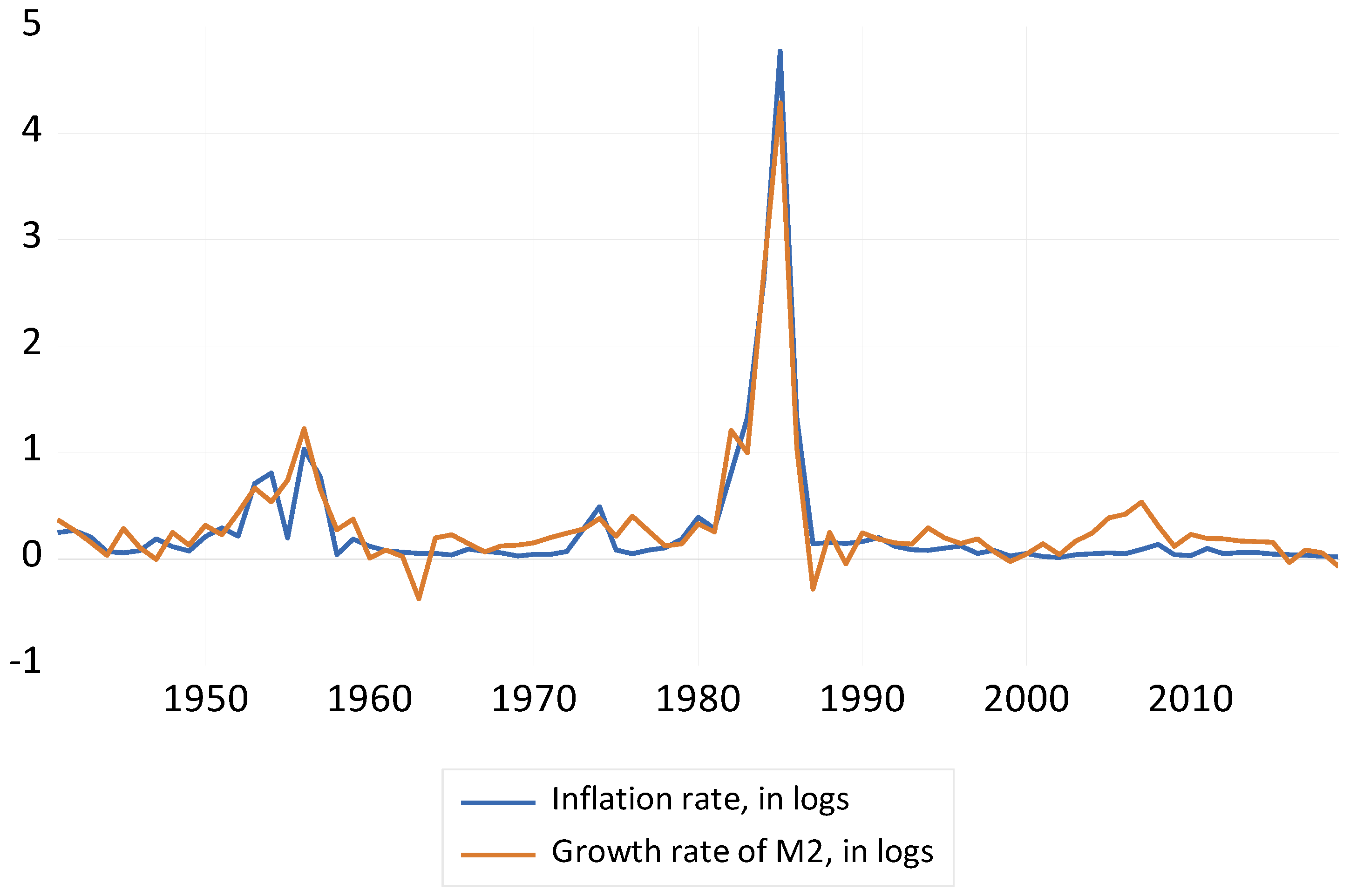
An immediate observation is that there is a visible positive correlation between inflation and the growth rate in M2—the correlation coefficient is +0.97—highlighting that, in Bolivia, these two variables go hand in hand, particularly during those periods where inflation is high. (The spike in inflation rates observed between 2007 and 2008 and 2010 and 2011 were the result of price increases in agricultural products in foreign markets. An appreciation of the Boliviano and contractionary monetary policies decreased inflation rates to target levels. Between 2013 and 2015, even though growth in GDP was high, the inflation rate decreased substantially.) Figure 1 corroborates this initial finding and shows that these two variables move very much in unison.

It is also noteworthy that inflation and real GDP growth are negatively correlated—the correlation coefficient is −0.38—but this negative relationship is not as visible if the hyperinflation years are excluded from the analysis. A preliminary conclusion from the decade-to-decade behavior of these variables is that there seem to be periods where the positive (negative) correlation between inflation and the growth rate in M2 (real GDP growth) is more visible, hence the necessity to analyze the relationship between these variables separating the high-inflation periods from the low-inflation ones.

4.1. Univariate Time-Varying Markov-Switching Model of Inflation

The process of inflation is first analyzed utilizing a time-varying univariate Markov-Switching model (TMS). Monthly inflation data have been available since 1937, hence the time-period covered is January 1937 through January 2020. The equation specification consists of a two-state Markov-switching model, with a single switching mean regressor C (the intercept) and four non-switching AR terms. The error variance is assumed to be common across the regimes and there are two probability regressors, the constant C and a one-period lag of the dependent variable since the model assumes time-varying regime transition probabilities. The inflation rate is expressed in natural logs. (Appendix A and Appendix B report results for the same specification when the inflation rate is expressed in percentages and when it is expressed as first differences of the natural log of the price level, respectively. The pattern of results is similar to the ones reported here.)

Table 2. Time-Varying Univariate Markov-Switching Model for Monthly Inflation.

	Regime 1—High Inflation		Regime 2—Low Inflation
	Coefficient	St. Error	Coefficient	St. Error
Switching Regressor
Constant	0.287 ***	0.011	0.015 *	0.008
# of Observations: 991
Log-Likelihood: 1830.549
Monthly Inflation Rate Expressed in Natural Logs
Probability Regressors: C, Inflationt−1, in Natural Logs
Four Non-Switching AR Regressors Included in Specification; not Shown in Table

* p < 0.1; ** p < 0.05; *** p < 0.01.

reports summarized results for regime 1 (high inflation) and regime 2 (low inflation).

As expected, the coefficient for C in regime 1 is significantly higher than in regime 2, implying that the expected mean value of inflation in the high inflation regime is higher than in the low inflation regime. Both coefficients are statistically significant, though at different levels of significance.

Table 3. Time-Varying Transition Probabilities and Expected Durations of Regime 1 and Regime 2.

Transition Probabilities: P(i, k) = P(s(t) = k | s(t−1) = i) (row = i/column = j)
		1	2
Mean	1	0.707	0.293
	2	0.021	0.979
		1	2
Std. Dev	1	0.047	0.047
	2	0.088	0.088
Expected Durations:
		1	2
Mean		3.46 months	139.00 months
Std. Dev.		0.354	557.451

presents the transition probability matrix and the expected duration of each regime.

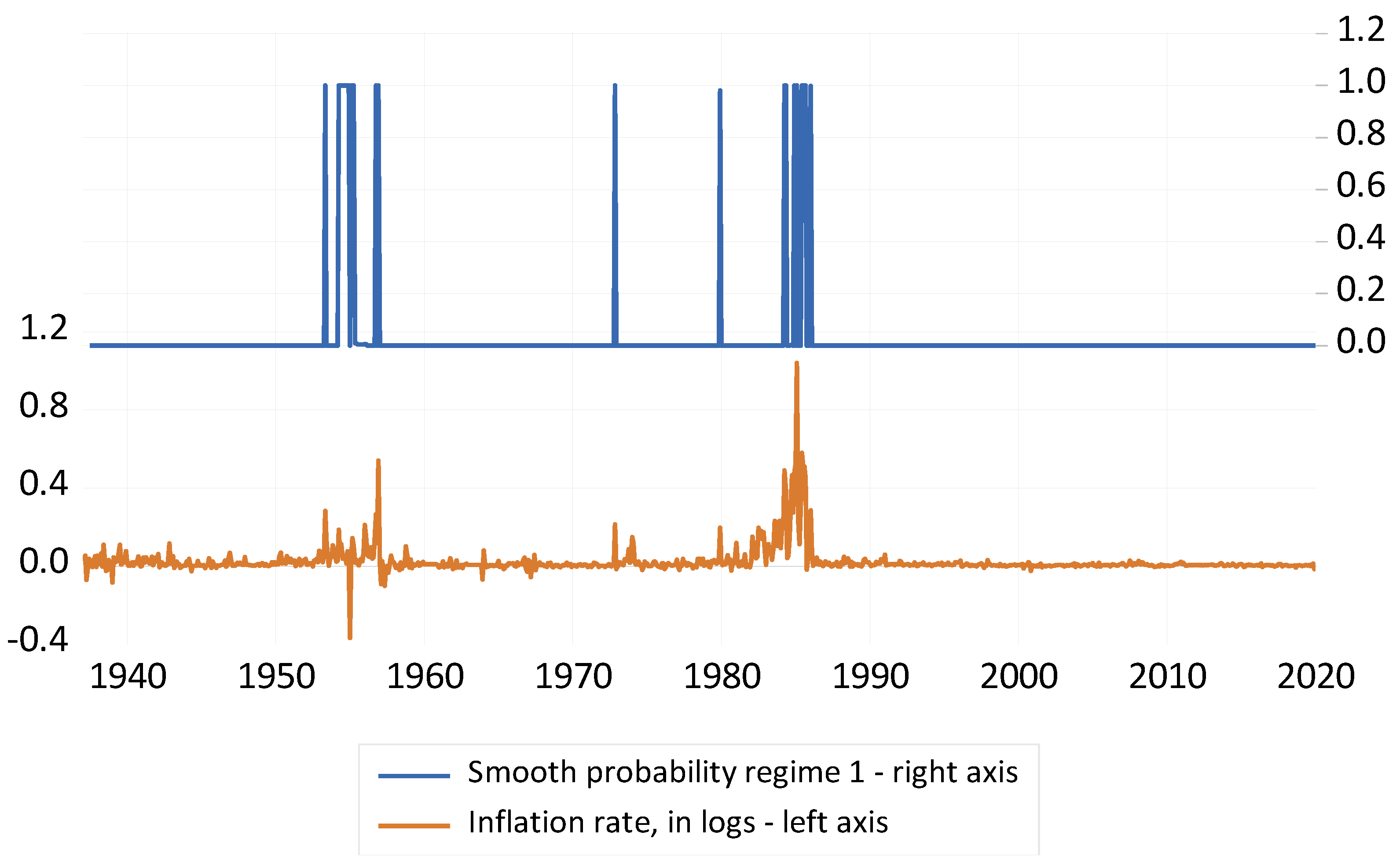
The results indicate that there is considerable state dependence in the transition probabilities, with a relatively higher probability of remaining in the low inflation regime (0.98 for the low inflation regime, 0.71 for the high inflation regime). The corresponding expected duration of each regime are 3.46 months (high inflation) and 139 months (low inflation). A visual summary of these findings is shown in Figure 2, where the smoothing probability of regime 1 (high inflation) is graphed along with the actual inflation rate. (Smoothed estimates for the regime probabilities in each period use the information set in the final period, in contrast to filtered estimates which employ only contemporaneous information. As Kim (1994) shows, using information about future realizations of the dependent variable improves the estimates of being in regime m in period t because the Markov transition probabilities link together the likelihood of the observed data in different periods.)

As is evident from Figure 2, the obtained probabilities reflect the comportment of the inflation rate. The high inflation regime (regime 1) nearly coincides with those months where the country experienced its highest inflation rates hence the close fit between what is predicted in the model and the actual evolution of prices during the entire period of interest. (The correlation coefficient between the smoothing probability of the high inflation regime and the monthly inflation rate (in logs) is +0.68).

4.2. Long Run, Multivariate Time-Varying Markov-Switching Model of Inflation

Utilizing yearly data for the period 1960–2018, the analysis of inflation from a long-run perspective is done by estimating a version of the quantity theory of money. Specifically, the standard quantity equation expressed in logs and in first differences is (Equation (4) is more appropriately defined as the equation of exchange. If it is assumed that the change in velocity is a random variable uncorrelated with money and real GDP growth, then the equation of exchange becomes the quantity theory of money):

$$\Delta m_t+\Delta v_t=\Delta p_t+\Delta y_t$$

(4)

where m is M2, v is velocity, p the price level, and y output. This can be rearranged as:

$$\Delta p_t=\Delta m_t+\Delta v_t-\Delta y_t$$

(5)

If it is assumed that in the long run both the money market and goods market are in equilibrium and that the trend of money velocity changes over time (Even though changes in the trend of money velocity are well documented—see, for instance, Bordon and Jonung (2004)—this might especially be true in Bolivia, where periods of severe price instability are not uncommon and where the unit of account has changed twice (in 1962 and in 1986) since the early 1960s. Velocity was estimated as follows: V = (nominal GDP)/M2, where both GDP and M2 are expressed in Bolivianos.) Then, framed as an unrestricted regression, the quantity theory becomes:

$${\pi }_t=C+{\beta }_1{X}_t+{\beta }_2{W}_t+{\beta }_3{Z}_t+{\epsilon }_t$$

(6)

where π_t represents yearly inflation; X_t, W_t, and Z_t represent growth rates in M2, velocity, and real GDP, respectively; and ε_t is a disturbance term with ${\epsilon }_t~\left(0,{\sigma }^2\right)$.

Equation (6) is estimated utilizing a two-state TMS model with four switching regressors (C and the growth rates, in natural logs, of M2, velocity, and real output) and one non-switching AR term. There are two probability regressors, the constant C and a one-period lag of the growth rate in M2. The latter is included so that the period t data for the regressor corresponds to the values influencing the transitions for t − 1 to t. The inflation rate is also expressed in natural logs.

Table 4. Time-Varying, Long-Run Multivariate Markov-Switching Model for Yearly Inflation.

	Regime 1—High Inflation		Regime 2—Low Inflation
	Coefficient	St. Error	Coefficient	St. Error
Switching Regressors
Constant	0.035	0.031	−0.038 ***	0.012
Growth Rate M2	1.026 ***	0.032	0.958 ***	0.010
Growth Rate Velocity	1.033 ***	0.154	1.026 ***	0.035
Growth Rate Real GDP	−1.786 ***	0.347	−0.025	0.245
R2	0.99		0.99
# of Observations: 57
Log-Likelihood: 102.885
All variables expressed in natural logs
Dependent variable: inflation rate
Probability regressors: C, (growth rate M2)t−1, in natural logs
One non-switching AR regressor included in specification; not shown in table

* p < 0.1; ** p < 0.05; *** p < 0.01.

reports summarized results for the high inflation and low inflation regimes.

The results for both regimes generally fall in line with what the quantity theory of money predicts. Money growth and velocity growth increase, and GDP growth reduces, inflation. Moreover, in the high inflation case, the coefficient for money growth is 1.026, which very much reflects the prediction of the theory that money growth increases inflation one-for-one. In the low-inflation regime, the coefficient is still positive but below 1, which is unsurprising since M2 includes a much broader range of assets than M1. In other words, in countries experiencing hyperinflation and negative real interest rates—as was the case in Bolivia between 1983–1986—people have an incentive to hold most M2 assets as currency (M1) to be spent promptly to minimize the inflation tax. If real interest rates are positive, however—as is presumably the case when inflation is low—the inflation tax would be minimized by holding the minimum feasible portion of M2 as currency for transactions, causing β₁ to be smaller than 1.

Real GDP growth is negative in both regimes but is statistically significant only in the high inflation case. Additionally, the coefficient, −1.786, is significantly smaller than the quantity theory prediction that β₃ = −1.0, a result that might partially be explained by the well-known challenges of measuring accurate output figures in countries similar to Bolivia. (See, for instance, Loayza (1997) work on the challenges faced by Latin American nations in measuring the size of the informal sector and its impact to growth and development.)

Table 5. Time-Varying Transition Probabilities and Expected Durations of Regime 1 and Regime 2.

Transition Probabilities: P(i, k) = P(s(t) = k | s(t−1) = i) (row = i/column = j)
		1	2
Mean	1	0.480	0.520
	2	0.368	0.632
Std. Dev	1	0.081	0.081
	2	0.296	0.296
Expected durations:
Mean		1.95 years	33.06 years
Std. Dev.		0.213	159.948

presents the transition probability matrix and the expected duration of each regime.

The results are similar to those obtained with the univariate TMS model. There is significant state dependence in the transition probabilities and there is a relatively higher probability of being in the low inflation regime (0.63 vs. 0.48 in the high inflation regime). Moreover, the expected durations of each regime are 1.95 years and 33.06 years for the high and low inflation regimes, respectively. These predictions are roughly in line with what happened to inflation during the 1960–2018 period: there were two years (1984 and 1985) where yearly inflation rates were above 1000 percent, and there were 38 years where inflation rates were below 10 percent. In the remaining 19 years, inflation rates exceeded 10 percent and fluctuated significantly, rising above 100 percent in 1982, 1983, and 1986.

Figure 3 shows the smoothing probability of regime 1 (high inflation) and the inflation rate.

As depicted in Figure 3, the obtained probabilities do not fit the actual evolution of the inflation rate as closely as the empirical findings suggest. (The correlation coefficient between the smoothing probability of the high inflation regime and the yearly inflation rate (in logs) is +0.11.) However, given the more volatile nature of inflation during the late 1960s, 1970s, the high-inflation 1980s, and the period after 2008, when inflation rates once again reach the two-digit mark, the observed pattern of behavior of the smoothing probabilities is unsurprising.

4.3. Short-Run, Multivariate Time-Varying Markov-Switching Model of Inflation

The standard expression for the short-run aggregate supply curve is:

$${\pi }_t={\pi }^e+\gamma \left(Y_t-Y^p\right)+{\epsilon }^{\pi }$$

(7)

where π_t is inflation at time t; π^e represents expected inflation; γ is a sensitivity factor; Y_t is output; Y^p stands for potential output (potential output was estimated utilizing the Hodrick–Prescott filter); and ε^π represents price shocks. The difference between Y_t and Y^p is referred to as the output gap and hence γ reflects how sensitive inflation is to fluctuations in the output gap.

If it is assumed that expectations are adaptive, then an appropriate indicator for expected inflation is past inflation. Additionally, if it is assumed that the country did not experience any significant price shocks, the short-run expression for inflation is:

$${\pi }_t={\pi }_{t-1}+\gamma \left(Y_t-Y^p\right)$$

(8)

where π_t−1 represents inflation in the previous period.

Formulated in regression form, Equation (8) becomes:

$${\pi }_t=C+{\beta }_1{X}_t+{\beta }_2{W}_t+{\epsilon }_t$$

(9)

and π_t represents yearly inflation; X_t stands for inflation in the previous period; W_t is the output gap; and ε_t is a disturbance term with ${\epsilon }_t~\left(0,{\sigma }^2\right)$.

Equation (9) is also estimated utilizing a two-state TMS model with three switching regressors (C, the log of inflation in the previous period, and the difference between the log of real GDP and the log of potential GDP) and one non-switching AR term. There are two probability regressors, the constant C and inflation in the previous period. Lagged inflation is included so that the period t data for the regressor corresponds to the values influencing the transitions for t − 1 to t. The dependent variable is also expressed in natural logs.

Table 6. Time-Varying, Short-Run Multivariate Markov-Switching Model for Yearly Inflation.

	Regime 1—High Inflation		Regime 2—Low Inflation
	Coefficient	St. Error	Coefficient	St. Error
Switching Regressors
Constant	0.786 **	0.371	0.048 ***	0.010
Previous Inflation (πt−1)	0.191	0.202	0.300 ***	0.099
Ouput Gap (Y − Yp)	−26.769 **	11.023	0.195	0.174
R2	0.33		0.01
# of Observations: 58
Log-Likelihood: 70.029
All variables expressed in natural logs
Dependent variable: inflation rate
Probability regressors: C, (previous inflation)t−1, in natural logs
One non-switching AR regressor included in specification; not shown in table

* p < 0.1; ** p < 0.05; *** p < 0.01.

reports summarized results for the high inflation and low inflation regimes.

The results indicate that in the high-inflation regime the most important determinant of inflation is a negative output gap, which occurs when actual output falls below potential output. Likewise, previous inflation does not have a statistically significant impact on current inflation, though β₁ does have the expected positive sign. In contrast, in the low-inflation regime, previous inflation is the most important predictor of current inflation—β₁ is positive and statistically significant—and the (positive) output gap does not seem to exert any influence. These results fit nicely with New Keynesian theory: during times of low inflation, nominal variables are sticky and hence current inflation depends on previous values of inflation. However, when prices no longer provide any useful information—as is the case during times of hyperinflation—past inflation plays no role in affecting current inflation. (The constant in regime 1 is significantly higher than in regime 2 and may, in part, justify why a negative output gap is the main determinant of inflation in the high-inflation regime. The constant prevents overall bias by forcing the residual mean to equal zero but may also capture the exclusion of relevant variables from the regression model. In the short run and during periods of high inflation, the standard expression for the short-run aggregate supply curve (Equation (8)) may include additional factors not considered here. Additionally, since specifications 7–9 aim to understand the principal variables that affect changes in the price level in the short run, perhaps a more appropriate indicator of inflation would be one where monthly changes in the price level are considered, rather than the yearly changes utilized here. Unfortunately, even though monthly inflation rates have been available since the late 1930s, there is no reliable monthly data on real GDP, which would be needed to estimate Equation (9). Not utilizing monthly data may also partly explain why inflation expectations do not play a more prominent role in the high-inflation regime.)

Table 7. Time-Varying Transition Probabilities and Expected Durations of Regime 1 and Regime 2.

Transition Probabilities: P(i, k) = P(s(t) = k | s(t−1) = i) (row = i/column = j)
		1	2
Mean	1	0.344	0.656
	2	0.183	0.817
Std. Dev	1	0.140	0.140
	2	0.340	0.340
Expected durations:
Mean		4.43 years	58.07 years
Std. Dev.		20.913	52.272

presents the transition probability matrix and the expected duration of each regime.

The results are consistent with previous findings. As was the case with univariate TMS and long-run multivariate TMS, there is significant state dependence on the transition probabilities, with a greater probability of being in the low-inflation regime (0.82) than in the high-inflation regime (0.34). The expected duration of each regime is 4.43 years and 58.07 years for the high and low inflation regimes, respectively, roughly resembling the pattern of behavior observed with the long run multivariate TMS model.

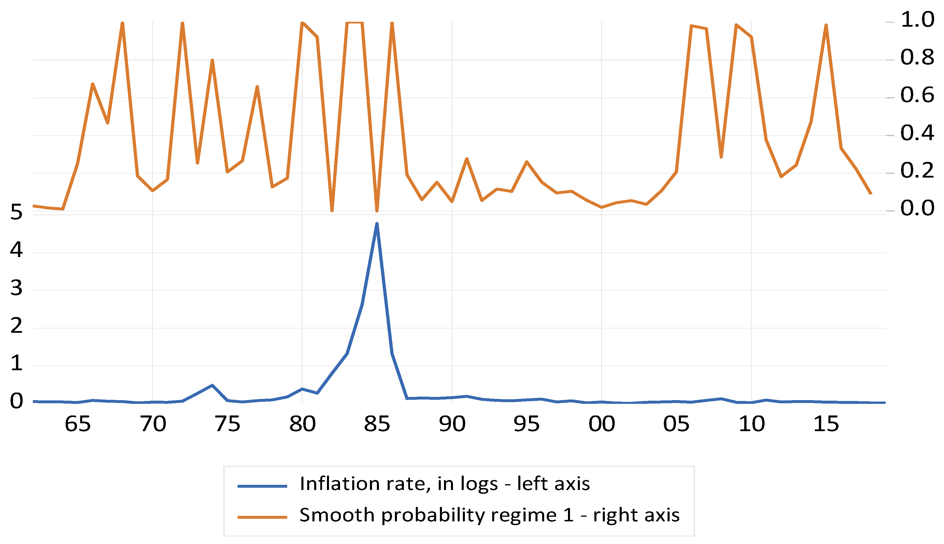
Figure 4 shows the smoothing probability of regime 1 (high inflation) and the inflation rate.

As depicted in Figure 4, the obtained probabilities closely fit the actual evolution of the inflation rate. (The correlation coefficient between the smoothing probability of the high inflation regime and the yearly inflation rate (in logs) is +0.68.) Years when there is a spike in inflation are echoed with rising smoothing probabilities, giving confidence that the empirical findings reflect fluctuations in the price level analyzed from a short-run perspective.

4.4. Partitioning the Sources of Inflation in the Long and Short-Run

Other things equal, the long-run multivariate TMS states that rapid money growth and velocity growth stimulate inflation, and real GDP growth mitigates it. Likewise, the short-run multivariate TMS contends that past inflation and the output gap determine inflation. However, what is the relative importance of each one of these variables in explaining inflation? Commonality analysis—a brief review is provided in Nathans et al. (2012)—is a method of decomposing the R² in a multiple regression analysis into the proportion of explained variance of the dependent variable associated with each independent variable.

For the long run multivariate TMS, the variance in the inflation rate explained by Equation (6) can be partitioned as:

$$V_{\pi }={\beta }_1^2{V}_x+{\beta }_2^2{V}_w+{\beta }_3^2{V}_z+2{\beta }_1{\beta }_2{V}_{xw}+2{\beta }_1{\beta }_3{V}_{xz}+2{\beta }_2{\beta }_3{V}_{wz}$$

(10)

where V_x, V_w, and V_z are the sample variances in X, W, and Z; V_xw is the sample covariance between X and W; V_xz is the sample covariance between X and Z; V_wz is the sample covariance between W and Z. The covariances between all combinations of the three variables are quite small, so the influences of money, velocity, and real GDP growth are nearly separate and additive. Substituting the regression coefficients from Table 4 and the sample variances V_x = 3.610; V_w = 17.510; V_z = 39.549; and covariances V_xw = 3.4 × 10⁻⁴; V_xz = 5.3 × 10⁻⁴; V_wz = 3.0 × 10⁻³, the explained regression variance for the high-inflation regime is:

V_π = 3.797 + 18.675 + 126.100 − 3.5 × 10⁻⁴ − 9.8 × 10⁻⁴ − 5.5 × 10⁻³ = 148.57

3.797 Explained by money growth; 18.675 Explained by velocity growth; 126.100 Explained by real GDP growth; 3.5 × 10⁻⁴ Explained jointly by money growth and velocity growth; 9.8 × 10⁻⁴ Explained jointly by money growth and real GDP growth; 5.5 × 10⁻³ Explained jointly by velocity growth and real GDP growth.

Likewise, the explained regression variance for the low-inflation regime is:

V_π = 1.023 + 4.174 + 0.017 − 1.2 × 10⁻⁴ − 1.4 × 10⁻⁵ − 8.5 × 10⁻⁶ = 5.21

In both cases, the covariances contribute almost nothing to explained regression variance. In the high-inflation regime, growth in real GDP contributes 126.10/148.57 = 0.849, or 84.9 percent of explained regression variance. Money growth contributes 3.797/148.57 = 0.026, or 2.6 percent, and velocity growth contributes 18.675/148.57 = 0.126, or 12.6 percent. In the low-inflation regime, the relative contributions of money growth, velocity growth, and real GDP growth are 19.64 percent, 80.12 percent, and 0.33 percent, respectively. Since the R² in both regimes is 0.99, the large differences in inflation are explained mostly by GDP growth in the high-inflation regime and by money growth and velocity growth in the low-inflation regime.

For the short run multivariate TMS, the variance in the inflation rate explained by Equation (9) can be partitioned as:

$$V_{\pi }={\beta }_1^2{V}_x+{\beta }_2^2{V}_w+2{\beta }_1{\beta }_2{V}_{xw}$$

(11)

where, as before, V_x and V_w are the sample variances in X and W, and V_xw is the sample covariance between X and W. The latter is quite small, so the influences of past inflation and the output gap are nearly separate and additive. Substituting the regression coefficients from Table 6 and the sample variances V_x = 23.469; V_w = 1278.638; and covariance V_xw = 0.417, the explained regression variance for the high-inflation regime is:

V_π = 0.856 + 916232.480 − 4.260 = 916229.076

Past inflation and the covariance of past inflation and the output gap contribute almost nothing to explained regression variance, but the variance explained by the output gap is enormous. Ignoring the others, the output gap explains 916,232.480/916,229.076 ≈ 1.0 or 100 percent of explained regression variance. Even though the R² is only 0.33, differences in inflation are explained almost entirely by differences in the output gap.

The explained regression variance for the low-inflation regime is:

V_π = 1.035 + 0.763 − 7.2 × 10⁻⁵ = 1.797

Past inflation contributes 1.035/1.797 = 0.576, or 57.6 percent of explained regression variance; the output gap contributes 0.763/1.797 = 0.424, or 42.4 percent; and the contribution of the covariance is nearly inexistent. With an R² of only 0.01, these results are taken with caution and no conclusions are drawn regarding the causes for differences in inflation in this regime.

5. Conclusions

Utilizing a time-varying univariate and multivariate Markov-switching model (TMS), the inflation process in Bolivia is described starting in the late 1930s. Having experienced at least two episodes of severe inflation in the 1950s and the 1980s, Bolivia stands alone as a country where a Markov process might very well be the right approach to analyze inflation.

The principal findings are these: with monthly data, the inflation process starting in 1937 is accurately described by a univariate TMS. The intercept for the high-inflation regime is significantly higher than for the low-inflation regime and the actual inflation rate mirrors the smoothing probabilities of the Markov process. Additionally, the predicted duration of each regime closely fits the periods when the country experienced low and inordinate high inflation rates.

From a long-run perspective and utilizing a multivariate TMS, the results generally fall in line with what the quantity theory of money predicts. In the high-inflation regime, money growth increases inflation (almost) one-for-one, as classical economics contends. Moreover, velocity growth increases, and real GDP growth decreases inflation, in accordance with expectations. In the low-inflation regime, both money growth and velocity are also positive and statistically significant, but real GDP growth is not, though it still has the predicted negative sign. The general conclusion is that inflation is a monetary phenomenon both in the high and low-inflation regimes, but the predictive power of how changes in the money supply affect inflation is clearer and closer to expectations in the high-inflation case. (There is a caveat to this conclusion. Even though growth in the money supply is a key determinant of inflation in both regimes, when the R² is decomposed to analyze the proportion of explained variance of the dependent variable associated with each independent variable, money growth is not the most important variable explaining inflation in either the high- or low-inflation regime.) The predicted expected duration of each regime is also aligned with the actual periods when the country experienced high and low inflation rates.

From a short-run perspective and utilizing a multivariate TMS, the findings indicate that in the high-inflation regime, inflation is almost exclusively explained by a negative output gap, though there is some indication that other factors might be at play. In the low-inflation regime, lagged inflation is the most important determinant of inflation, in line with price stickiness expectations. Unsurprisingly, in the high-inflation regime, lagged inflation is statistically insignificant, showing that, when prices no longer provide useful information, past price fluctuations play no role in affecting current inflation. Graphical analysis of smoothing probabilities and actual inflation rate demonstrate the accuracy of the empirical estimates and the predicted expected duration of both regimes align with the actual evolution of prices during the period of interest.

Partitioning the sources of inflation demonstrate that, from a long-run perspective and in the high inflation regime, differences in inflation are mostly explained by GDP growth; likewise, in the low-inflation regime, money growth and velocity growth are the principal factors explaining the variance of inflation. From a short-run perspective, the output gap explains almost all regression variance in the high-inflation regime, and past inflation does the same during times of low inflation, though in both cases the R² is low, which precludes making definite statements about the sources of variability in inflation.

An important conclusion is that, in countries such as Bolivia, that have experienced significant price fluctuations, inflation is best analyzed with models that allow for changes in the parameters affecting it over a set of different unobserved states. The results are likely to incorporate specific features of each state and hence generate more reliable estimates of the factors that affect inflation over time.

The principal policy implication concerns control of the money supply. Since it has been determined that from a long-run perspective the growth rate in M2 is a principal determinant of inflation both in high- and low inflation regimes, then it is up to the Bolivian Central Bank to make sure that the money supply does not grow out of hand. Further, and from a short-run perspective, restricting the growth in the money supply may also dampen inflationary expectations, which has been found to be an important determinant of inflation in the low-inflation regime.

References

- Acharya, Viral V., and Lasse Heje Pedersen. 2005. Asset Pricing with Liquidity Risk. Journal of Financial Economics 77: 375–410. [Google Scholar] [CrossRef] [Green Version]
- Aït-Sahalia, Yacine. 1996. Testing Continuous-Time Models of the Spot Interest Rate. Review of Financial Studies 9: 385–426. [Google Scholar] [CrossRef]
- Alexander, Carol, and Andreas Kaeck. 2008. Regime Dependent Determinants of Credit Default Swap Spreads. Journal of Banking and Finance 32: 1008–21. [Google Scholar] [CrossRef]
- Amisano, Gianni, and Gabriel Fagan. 2013. Money Growth and Inflation: A Regime Switching Approach. Journal of International Money and Finance 33: 118–45. [Google Scholar] [CrossRef] [Green Version]
- Ascari, Guido, Louis Phaneuf, and Eric R. Sims. 2018. On the Welfare and Cyclical Implications of Moderate Trend Inflation. Journal of Monetary Economics 99: 56–71. [Google Scholar] [CrossRef] [Green Version]
- Aye, Goodness C., Tsangyao Chang, and Rangan Gupta. 2016. Is Gold an Inflation-Hedge? Evidence from an Interrupted Markov-Switching Cointegration Model. Resources Policy 48: 77–84. [Google Scholar] [CrossRef] [Green Version]
- Bidarkota, Prasad V. 2001. Alternative Regime Switching Models for Forecasting Inflation. Journal of Forecasting 20: 21–35. [Google Scholar] [CrossRef]
- Binner, Jane M., C. Thomas Elger, Birger Nilsson, and Jonathan A. Tepper. 2006. Predictable Non-Linearities in US Inflation. Economics Letters 93: 323–28. [Google Scholar] [CrossRef] [Green Version]
- Bojanic, Antonio N. 2013. Inflación e Incertidumbre Inflacionaria en Bolivia. El Trimestre Económico 80: 401–26. [Google Scholar] [CrossRef] [Green Version]
- Bojanic, Antonio N. 2019. Evolution of the Bolivian Economy, 2nd ed. Dubuque: Kendall Hunt Publishing Company. [Google Scholar]
- Bordon, Michael D., and Lars Jonung. 2004. Demand for Money: An Analysis of the Long-Run Behavior of the Velocity of Circulation. Piscataway: Transaction Publishers. [Google Scholar]
- Cabrieto, Jedelyn, Janne Adolf, Francis Tuerlinckx, Peter Kuppens, and Eva Ceulemans. 2018. Detecting Long-Lived Autodependency Changes in a Multivariate System Via Change Point Detection and Regime Switching Models. Scientific Reports 8: 15637. [Google Scholar] [CrossRef] [PubMed]
- Campbell, John, and John Cochrane. 1999. By Force of Habit: A Consumption-Based Explanation of Aggregate Stock Market Behavior. Journal of Political Economy 107: 205–51. [Google Scholar] [CrossRef]
- Dai, Wei, and Apostolos Serletis. 2019. On the Markov Switching Welfare Cost of Inflation. Journal of Economic Dynamics and Control 108: 103748. [Google Scholar] [CrossRef] [Green Version]
- Davig, Troy, and Taeyoung Doh. 2014. Monetary Policy Regime Shifts and Inflation Persistence. Review of Economics and Statistics 96: 862–75. [Google Scholar] [CrossRef] [Green Version]
- Di Persio, Luca, and Samuele Vettori. 2014. Markov Switching Model Analysis of Implied Volatility for Market Indexes with Applications to S&P 500 and DAX. Journal of Mathematics 2014: 753852. [Google Scholar] [CrossRef]
- Diebold, Francis X., Joon-Haeng Lee, and Gretchen C. Weinbach. 1994. Regime Switching with Time-Varying Transition Probabilities. In Nonstationary Time Series Analysis and Cointegration. Edited by Colin Hargreaves. Oxford: Oxford University Press, pp. 283–302. [Google Scholar]
- Driffill, John, and Martin Sola. 1998. Intrinsic Bubbles and Regime-Switching. Journal of Monetary Economics 42: 353–73. [Google Scholar] [CrossRef]
- Engel, Charles. 1994. Can the Markov Switching Model Forecast Exchange Rates? Journal of International Economics 36: 151–65. [Google Scholar] [CrossRef] [Green Version]
- Filardo, Andrew J. 1994. Business-Cycle Phases and Their Transitional Dynamics. Journal of Business & Economic Statistics 12: 299–308. [Google Scholar]
- Fink, Holger, Yulia Klimova, Claudia Czado, and Jakob Stöber. 2017. Regime Switching Vine Copula Models for Global Equity and Volatility Indices. Econometrics 5: 3. [Google Scholar] [CrossRef] [Green Version]
- Friedman, Milton. 1963. Inflation: Causes and Consequences, Collected Works of Milton Friedman Project Records, Hoover Institution Archives. Available online: https://miltonfriedman.hoover.org/objects/57545 (accessed on 3 July 2020).
- Goldfeld, Stephen M., and Richard E. Quandt. 1973. A Markov Model for Switching Regressions. Journal of Econometrics 1: 3–15. [Google Scholar] [CrossRef]
- Guerson, Alejandro. 2015. Inflation Dynamics and Monetary Policy in Bolivia, IMF Working Paper WP/15/266. Available online: https://ssrn.com/abstract=2733575 (accessed on 3 July 2020).
- Hamilton, James D. 1989. A New Approach to the Economic Analysis of Nonstationary Time Series and the Business Cycle. Econometrica 57: 357–84. [Google Scholar] [CrossRef]
- Hamilton, James D. 2005. What’s Real about the Business Cycle? Federal Reserve Bank of St. Louis Review 87: 435–52. [Google Scholar]
- Hamilton, James D. 2016. Macroeconomic Regimes and Regime Shifts. In Handbook of Macroeconomics. Edited by Harald Uhlig and John Taylor. Amsterdam: Elsevier, vol. 2A, pp. 163–201. [Google Scholar]
- Kim, Chang-Jin, Jeremy Piger, and Richard Startz. 2008. Estimation of Markov Regime-Switching Regression Models with Endogenous Switching. Journal of Econometrics 143: 263–73. [Google Scholar] [CrossRef] [Green Version]
- Kim, Chang-Jin. 1993a. Unobserved-Component Time Series Models with Markov-Switching Heteroscedasticity: Changes in Regime and the Link between Inflation Rates and Inflation Uncertainty. Journal of Business & Economics Statistics 11: 341–49. [Google Scholar]
- Kim, Chang-Jin. 1993b. Sources of Monetary Growth Uncertainty and Economic Activity: The Time-Varying-Parameter Model with Heteroskedastic Disturbances. The Review of Economics and Statistics 75: 483–92. [Google Scholar] [CrossRef]
- Kim, Chang-Jin. 1994. Dynamic Linear Models with Markov-Switching. Journal of Econometrics 60: 1–22. [Google Scholar] [CrossRef]
- Loayza, Norman A. 1997. The Economics of the Informal Sector: A Simple Model and Some Empirical Evidence from Latin America (English). Policy, Research Working Paper, No. WPS 1727. Washington: World Bank Group, Available online: http://documents.worldbank.org/curated/en/685181468743710751/The-economics-of-the-informal-sector-a-simple-model-and-some-empirical-evidence-from-Latin-America (accessed on 3 July 2020).
- Lucas, Robert E. 2000. Inflation and Welfare. Econometrica 68: 247–74. [Google Scholar] [CrossRef]
- Ma, Feng, M. I. M. Wahab, Dengshi Huang, and Weiju Xu. 2017. Forecasting the Realized Volatility of the Oil Futures Market: A Regime Switching Approach. Energy Economics 67: 136–45. [Google Scholar] [CrossRef]
- Maheu, John M., and Thomas H. McCurdy. 2002. Nonlinear Features of Realized FX Volatility. Review of Economics and Statistics 84: 668–81. [Google Scholar] [CrossRef]
- Montero Kuscevic, Casto Martín, Marco Antonio del Río Rivera, and J. Sebastian Leguizamon. 2018. Inflation Volatility and Economic Growth in Bolivia: A Regional Analysis. Macroeconomics and Finance in Emerging Market Economies 11: 36–46. [Google Scholar] [CrossRef]
- Morales, Juan Antonio. 1987. Inflation Stabilization in Bolivia, Documento de Trabajo No. 06/87. La Paz: Universidad Católica Boliviana, Instituto de Investigaciones Socio-Económicas (IISEC). [Google Scholar]
- Moroney, John R. 2002. Money Growth, Output Growth, and Inflation: Estimation of a Modern Quantity Theory. Southern Economic Journal 69: 398–413. [Google Scholar] [CrossRef]
- Nathans, Laura L., Frederick L. Oswald, and Kim Nimon. 2012. Interpreting Multiple Linear Regression: A Guidebook of Variable Importance. Practical Assessment, Research, and Evaluation 17: 9. [Google Scholar] [CrossRef]
- Penha Cysne, Rubens, and Davis Turchick. 2010. Welfare Costs of Inflation when Interest-Bearing Deposits are Disregarded: A Calculation of the Bias. Journal of Economic Dynamics and Control 34: 1015–30. [Google Scholar] [CrossRef]
- Rapach, David E., and Mark E. Wohar. 2005. In-Sample vs. Out-of-Sample Tests of Stock Return Predictability in the Context of Data Mining. Journal of Empirical Finance 13: 231–47. [Google Scholar] [CrossRef]
- Sachs, Jeffrey. 1986. The Bolivian Hyperinflation and Stabilization. NBER Discussion Paper Series No. 2073. Cambridge: NBER. [Google Scholar]
- Simon, John. 1996. A Markov-Switching Model of Inflation in Australia. RBA Research Discussion Papers, rdp9611. Sydney: Reserve Bank of Australia. [Google Scholar]
Figure 1.
Yearly Inflation Rate and Growth Rate of M2, 1941–2019. Sources: Central Bank of Bolivia; Bojanic (2019).
Figure 2.
Smoothing Probability of Regime 1 (high inflation) and Monthly Inflation Rate.
Figure 3.
Long Run, Smoothing Probability of Regime 1 and Yearly Inflation Rate.
Figure 4.
Short Run, Smoothing Probability of Regime 1 and Yearly Inflation Rate.