1. Introduction
Over the past decade, integrated volatility and jumps in asset pricing have attracted particular attention in the literature of finance, and their importance is prominent (
Brownlees et al. 2020;
Buncic and Gisler 2017). As per the efficient market hypothesis (EMH), the stock market responds to the arrival of new information, leading to changes in returns and volatility of the stock market prices (
Duangin et al. 2018). However, sometimes there are abnormal movements or large discontinuous changes in stock prices, which are infrequent but large; these extreme movements are known as jumps, associated with the arrival of unexpected new information (
Ferriani and Zoi 2020;
Jiang and Zhu 2017;
Sun and Gao 2020). Accordingly to
Bajgrowicz et al. (
2016), jumps are related to macroeconomic news, prescheduled company-specific announcements, and news reports that included a variety of unscheduled and uncategorized events. The vast majority of news does not cause price jumps, but it may give rise to a market reaction in the form of bursts of volatility.
Merton (
1976) first introduced price jumps in his seminal paper, starting an extensive strand of literature in asset pricing and financial econometrics. Jumps identification has profound implications in risk management, asset pricing, valuation of derivatives, and portfolio allocation (
Aït-Sahalia 2004;
Bajgrowicz et al. 2016;
Brownlees et al. 2020;
Odusami 2021;
Zhang et al. 2020).
Odusami (
2021) stated that it is essential to include jumps in financial models for managing the risk in the portfolio because jumps bring movements in asset prices; therefore, risk premia should be accounting for jumps along with continuous sample path variance. This study has observed asymmetry in the distribution of jumps, with a higher magnitude of negative jumps than positive jumps. The implication of their study is that jump risk is non-diversifiable. Therefore, when pricing assets, investors should account for risk premia, and when selecting policy weights in their portfolios, they should consider the determinants of jump risks.
Zhang et al. (
2020) documented that in China, most of the listed companies are owned by the state and a limited portion of shares are available for trading in the stock market. Therefore, the Chinese stock market is highly susceptible to speculation. Furthermore, due to the increasing role of domestic and foreign institutions, stock market movements are still primarily driven by noise traders; that is, retail investors. Therefore, more jumps could be expected in emerging markets such as the Chinese stock market than in the developed stock markets.
The importance of jumps is illustrated in some early studies, including by
Aït-Sahalia (
2004),
Aït-Sahalia and Hurd (
2015),
Amaya and Vasquez (
2011),
Nguyen et al. (
2019),
Buncic and Gisler (
2017),
Carr and Wu (
2003),
Duangin et al. (
2018),
Dutta et al. (
2020),
Eraker et al. (
2003),
Ferriani and Zoi (
2020),
Jiang and Oomen (
2008),
Jiang and Yao (
2013),
Jiang and Zhu (
2017),
Pan (
2002), and
Wright and Zhou (
2009).
Pan (
2002) shows evidence that investors demand a higher risk premium for taking the risk associated with price jumps.
Eraker et al. (
2003) found strong evidence for jumps in returns and jumps in volatility. Jumps in the volatility model significantly increase implied volatility in the money and out of the money options than models having only jumps in returns.
Carr and Wu (
2003) state that to understand asset price behavior, it is necessary to determine whether the best model is based on a purely continuous process, a pure jump process, or a combination of both of these two processes.
Aït-Sahalia (
2004) comments that jumps play an important role in asset returns, diminishing marginal returns, currencies, and interest rates. Moreover, the decomposition of total risk into Brownian and jump components is very useful for portfolio allocation and risk management.
Jiang and Oomen (
2008) document that jumps are an essential component of financial asset price dynamics. The arrival of unanticipated news or liquidity shocks often results in substantial and instantaneous revisions in the valuation of financial securities.
Wright and Zhou (
2009) explained that there is significant evidence of predictability in excess returns on various assets, and some of the predictability may be attributed to time-variation in the distribution of jump risk. They observed that jump risk measures could accurately predict future excess returns of the bond. Furthermore, the coefficient on the jump means it is statistically significant, implying that including jumps can increase the predictability of bond risk premia. The analysis has shown that root mean square prediction error can be reduced to 40% by including the jump mean in the model.
Amaya and Vasquez (
2011) suggest that positive jumps have a different effect on the future price of stocks than negative jumps. Positive jumps increase the prices of securities, and thus, a risk-averse investor prefers a positive over a negative jump. Therefore, stocks with negative jumps should earn a premium compared to stocks with positive jumps.
Jiang and Yao (
2013) stated that small and illiquid stocks have higher jump returns and the value premium is accounted for by the jumps.
Jiang and Zhu (
2017) using jumps as a proxy of informational shocks relaxed the requirements of planned event dates; therefore, they are not strictly related to events that are announced publicly. Jumps carry information that is beyond specific planned corporate events and bring large discontinued changes in the prices.
Corradi et al. (
2018) argued that considering the jump behavior improves the conditional variance forecasts of returns.
Ferriani and Zoi (
2020) noted that during phlegmatic market conditions, the relative contribution of jumps to total price variance is higher than during times of stress.
Dutta et al. (
2020) tested the presence of jumps in OVX and explored their role to predict crude oil price volatility. According to the findings, OVX has a jump behavior that varies over time. They warrant investors, policymakers, and academics accounting for the presence of jumps to develop more accurate asset pricing models and volatility prediction methods.
Baker et al. (
2020) explored the possible explanations for the stock market’s unusual reaction to the COVID-19 pandemic. Previous pandemics had a very mild impact on the US stock market, whereas the COVID-19 pandemic has had a much more substantial impact on the stock market than previous pandemics such as the Spanish flu. The evidence suggests that government restrictions on commercial activity and voluntary social distancing, operating with powerful effects in a service-oriented economy, are the primary reasons that the US stock market reacted so strongly to COVID-19 than to the previous pandemic.
Sharif et al. (
2020) examined the relationship between COVID-19, oil price volatility shock, the stock market, geopolitical risk, and economic policy uncertainty using the coherence wavelet method and wavelet-based Granger causality tests. It is found from the analysis that COVID-19 and oil price shocks have an impact on geopolitical risk levels, economic policy uncertainty, and stock market volatility over low-frequency bands.
Apergis and Apergis (
2020) analyzed the impact of the COVID-19 pandemic on the returns and volatility of the Chinese stock market. For COVID-19, they used two proxies: the total confirmed cases and the total daily deaths. The analysis shows that COVID-19, as measured by two different proxies, has a significant negative impact on stock returns; however, when total deaths are used as a proxy, the negative impact on stock returns is more pronounced. COVID-19, on the other hand, has a positive and statistically significant effect on the volatility. The findings are important for understanding the stock market implications of the COVID-19 pandemic.
Uddin et al. (
2021) studied the impact of the COVID-19 pandemic on stock market volatility to see if economic strength could help mitigate the negative effects of the global pandemic. According to the findings, country-level economic characteristics and factors help to mitigate the volatility caused by the pandemic. Based on economic factors, policymakers may devise policies to combat stock market volatility and avoid financial crises in the future. Empirical results of
Kostrzewski and Kostrzewska (
2021) indicate that a model with a time-varying jump intensity and a jump prediction mechanism is useful in forecasting.
A comprehensive study is needed to cover the existing gap in the literature related to the jump studies. As stated by
Kongsilp and Mateus (
2017), most existing studies on jump behavior are based on the developed market, whereas
Zhang et al. (
2020) stated that there are very few studies on jump behavior in the emerging market. We have conducted this study to cover the gap; first, by identifying jumps in Asian developed and emerging markets and to compare both markets. Second, to study asymmetric behaviour of positive and negative jumps in returns of Asian developed and emerging markets and to compare both markets. Third, to study asymmetric behavior of positive and negative jumps in integrated volatility of Asian emerging and developed markets and to compare their results.
This study aims to examine whether jumps matter in equity market returns and integrated volatility in the context of Asian developed and emerging equity markets.
The contribution of this paper is as follows. First, we apply the swap variance (SwV) test developed by
Jiang and Oomen (
2008) to identify monthly jumps in Asian developed markets and Asian emerging markets. The SwV test is similar in purpose to the bi-power variation (BPV) test developed by
Barndorff-Nielsen and Shephard (
2006) but with different logic and properties. The BPV test identifies jumps by comparing RV to a jump robust variance measure. In contrast, the SwV test identifies jumps by comparing RV to a jump-sensitive variance measure involving higher-order moments of returns, making it more powerful in many circumstances. Moreover, the SwV jump test explicitly considers market microstructure noise and can be applied to daily data (
Jiang and Oomen 2008;
Jiang and Zhu 2017). Second, we examine the role of positive jumps and negative jumps in equity returns individually and collectively. Third, we identify the role of positive and negative jumps in integrated volatility separately and jointly. The study further provides insight into the varying dynamics of jumps in developed and emerging markets of Asia. The findings in our study provide insights to academics, practitioners, and policymakers on the asymmetric effect of jumps in equity market returns and integrated volatility in the context of developed and emerging markets.
The rest of the paper is organized as follows.
Section 2 is a methodological review of the swap variance jump,
Section 3 explains the theory,
Section 4 describes the data and methodology,
Section 5 provides empirical results and findings,
Section 6 discusses the results with previous studies, whereas
Section 7 concludes the study and provides future directions.
2. Methodological Review of Swap Variance Jump
Andersen et al. (
2001,
2003b) proposed realized volatility (RV). RV is a model-free and error-free estimator of integrated volatility in the absence of noise and jumps.
Barndorff-Nielsen and Shephard (
2003) extended RV and introduced a generalized form of realized volatility known as realized power variation (RPV). Based on RPV,
Barndorff-Nielsen and Shephard (
2004) introduce realized bi-power variation (BPV), which is a partial generalization of quadratic variation. BPV has the same robustness property as RPV. However, BPV also estimates the integrated variance in stochastic volatility models. In this way, BPV provides a model-free and consistent alternative to realized variance.
Barndorff-Nielsen and Shephard (
2004) also introduced the generalized form of bi-power variation called tri-power variation (TPV). BPV was an unbiased estimator of integrated volatility in the presence of jumps, but it is subject to an upward bias in a finite sample. TPV is more efficient than BPV but also more vulnerable to market microstructure noise of high-frequency data.
Eraker et al. (
2003) developed a likelihood-based estimation method and analyzed jumps in returns and jumps in volatility in the S&P 500 and Nasdaq 100 index. Empirics shows strong evidence for jumps in returns and jumps in volatility.
Andersen et al. (
2003a) developed a non-parametric technique to measure continuous sample path variation and discontinuous (the jump part) of a quadratic variation process separately. It was found that the jump component is less persistent than the continuous sample path. The coefficient of the jump component is highly significant in daily, weekly, and quarterly forecast horizons. This study shows that financial asset allocation, risk management, and derivatives pricing can be improved by separating the model for continuous and jump components.
Carr and Wu (
2003) argued that it is essential to know whether it is the best model by using a purely continuous model, a pure jump process, or a combination of both of these two processes to understand asset prices’ behavior. They developed a method to differentiate between these processes. They examined these processes using market prices of at-the-money (ATM) and out-of-the-money (OTM) options as the option maturity date approaches the valuation date. The speed of convergence varies across these possibilities when ATM and OTM options prices converge to zero as the maturity date approaches zero. They identified the type of asset price process by examining the convergence speed of the option prices. In a continuous process, there are low chances that the underlying asset prices will jump by a large amount over a short time interval. So there is a small possibility that the OTM option will move in the money. Whereas, in the jump process, there are high chances that the underlying asset prices can jump into the money in a short period. The behavior of these two types of processes is different for option prices in the short term because these two processes are difficult to distinguish from a discretely sampled path.
Johannes (
2004) explores the statistical and economic role of jumps in continuous-time interest rate models. The results show that jumps are substantial both economically and statistically. Statistically, the presence of jumps means that models of diffusion are misspecified. Diffusion models ignore jumps and are incorrectly specified because the tail behavior of interest rate changes cannot be accurately captured. To quantify the statistical role of jumps in interest rates, he proposed and estimated a non-parametric jump-diffusion model.
Aït-Sahalia (
2004) uses maximum likelihood statistical-based methods to disentangle volatility from jumps accurately. He decomposes total noise into a continuous Brownian part and a discontinuous jump part. The Levy process is the sum of three independent Levy processes, which are a continuous component (Brownian motion), a component of big jumps in the form of a compound Poisson process with jump size larger than one, and a component of small jumps in the form of a pure martingale jump with jump size smaller than one. In this paper, Aït-Sahalia separated the Brownian component from the big jumps component and disentangled the Brownian component from the small jumps components.
Barndorff-Nielsen and Shephard (
2004) concluded that the probability limit of the bi-power estimator does not change by adding jumps to the SV model, meaning that realized variance can be combined with realized bi-power variation to estimate the quadratic variation of the jump component (the difference between realized variance and realized bi-power variation). This method separates quadratic variation into its continuous and jump components.
Barndorff-Nielsen and Shephard (
2006) propose two tests of jumps identification. One is the difference, and the second measure is the ratio of realized BPV and realized quadratic variation. They build the jump test on the idea of bi-power variation (BPV) provided by
Barndorff-Nielsen and Shephard (
2004) and
Back (
1991) that the sum of squared returns, a measure of variations in asset prices, is based on the quadratic variation process.
Lee and Mykland (
2008) proposed a jump detection technique and conducted an empirical study on US equity markets. It found that more frequent jumps are observed in individual equity returns, and their size is larger than the index returns. In individual stocks, jumps are associated with company-specific news, i.e., scheduled earnings announcements and unscheduled news. Therefore, with earnings announcements, other firm-specific news is to be incorporated for option pricing. Whereas in the index, jumps occur because of general market news, i.e., Federal Open Market Committee (FOMC) meetings and macroeconomic reports. Therefore, general market news is to be incorporated for index options.
Jiang and Oomen (
2008) established a non-parametric test to identify jumps in stock prices, known as the swap-variance (SwV) approach. They built their test from the concept of
Neuberger’s (
1994) variance swap replication strategy—a short position in the log contract plus a continuously rebalanced long position in the swap contract. The profit/loss of such a replication strategy will accumulate to an amount proportional to the variance realized (RV) and, as such, allows the swap contract to be perfectly replicated. Such a strategy fails, though, with jumps, and the realized jumps fully determine the replication error. The accumulated difference between simple returns and log returns is calculated—a quantity called “swap variance”—and compared to RV.
The difference will be indistinguishable from zero when jumps are absent, but when jumps are present, it will reflect the variance swap replication error, which in turn, lends its power to detect jumps. This test is similar in purpose to
Barndorff-Nielsen and Shephard’s (
2006) bi-power variation test, but with different underlying logic and properties. By contrasting RV to a jump robust variance measure, the BPV test identifies jumps. By comparing RV to a jump-sensitive variance measure involving higher-order moments of return, the SwV test identifies jumps, making it more powerful in many circumstances. They conducted extensive simulations to examine the performance of the SwV test and compared their results with the bi-power variation test. The results indicate that the SwV jump test performs well and is a useful addition to the bi-power variation test.
5. Empirical Analysis
Table 1 shows the number of months in which jumps have been identified. In the developed markets, it is observed that the Hang Seng index has the maximum number of jumps. The jumps have been identified in 71 months out of 229 months being studied, including 43 positive jumps and 28 negative jumps. Furthermore, the minimum number of jumps in the developed markets are identified in NZX50, which are in 56 months out of a total of 229 months. In these 56 months, 33 months have positive jumps, whereas 23 months have negative jumps.
In the emerging markets, the maximum number of jumps are identified in the CSE All index, which has jumps in 100 months with 63 positive jumps and 37 negative jumps. However, the minimum number of jumps is 63 for the Nifty50 index, including 40 positive jumps and 23 negative jumps.
It is concluded from
Table 1 that, on average, the developed markets have fewer jumps as compared with the emerging markets. Similarly, positive and negative jumps also arise more frequently in the emerging markets in comparison with the developed markets. Furthermore, on average, the tendency of a larger number of positive jumps relative to negative jumps occurs in both developed and emerging markets.
The possible justifications of the occurrence of more jumps in the emerging markets relative to the developed markets could be the riskier and more volatile nature of the emerging markets due to political instability, poor corporate governance, thin structure of the markets, lack of liquidity, high inflation rate, deflation or currency devaluations, interest rate risk, and high cross-border cash flows. All these factors hurt the economy and make the stock markets highly volatile, which leads to an increase in the tendency of jumps.
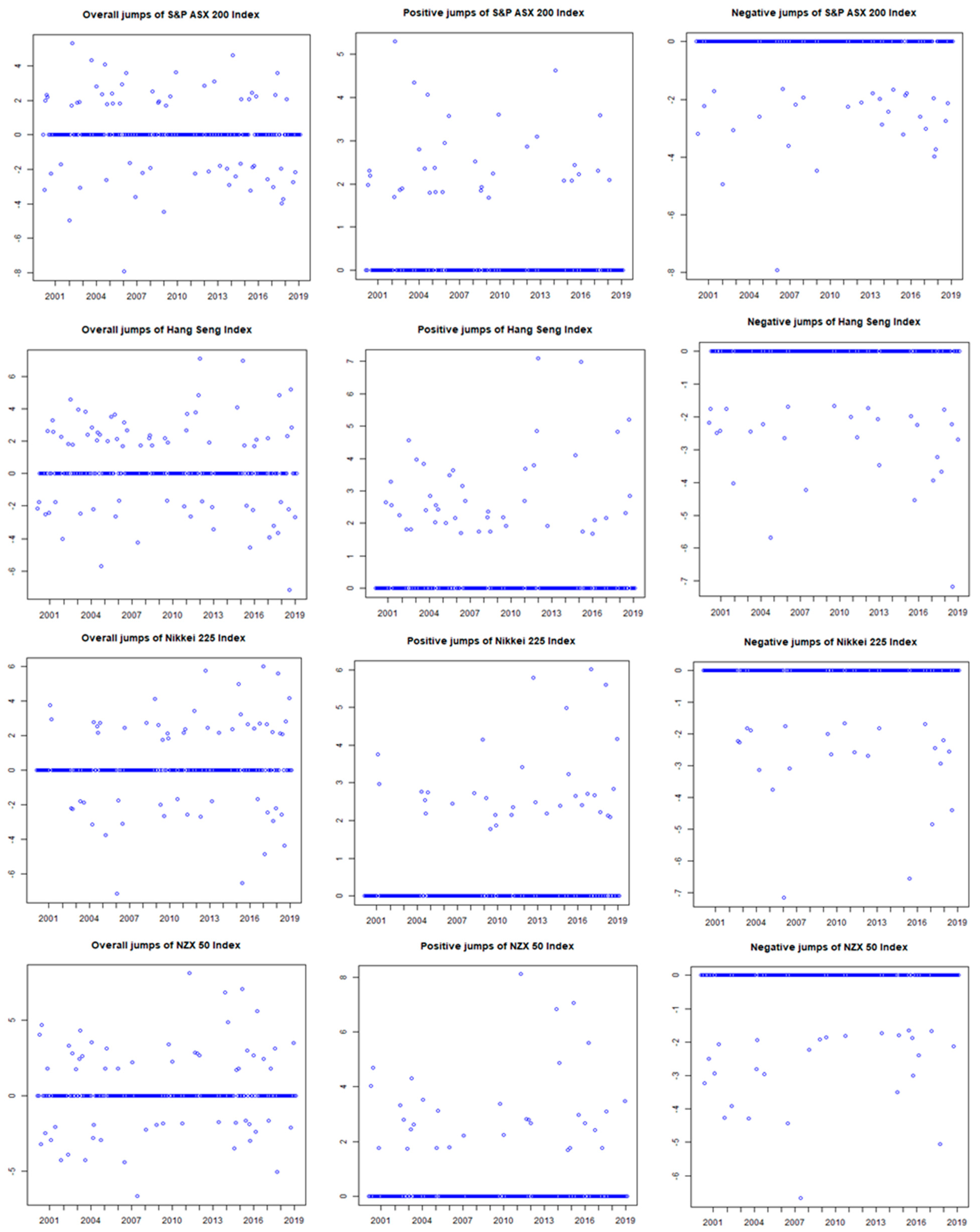
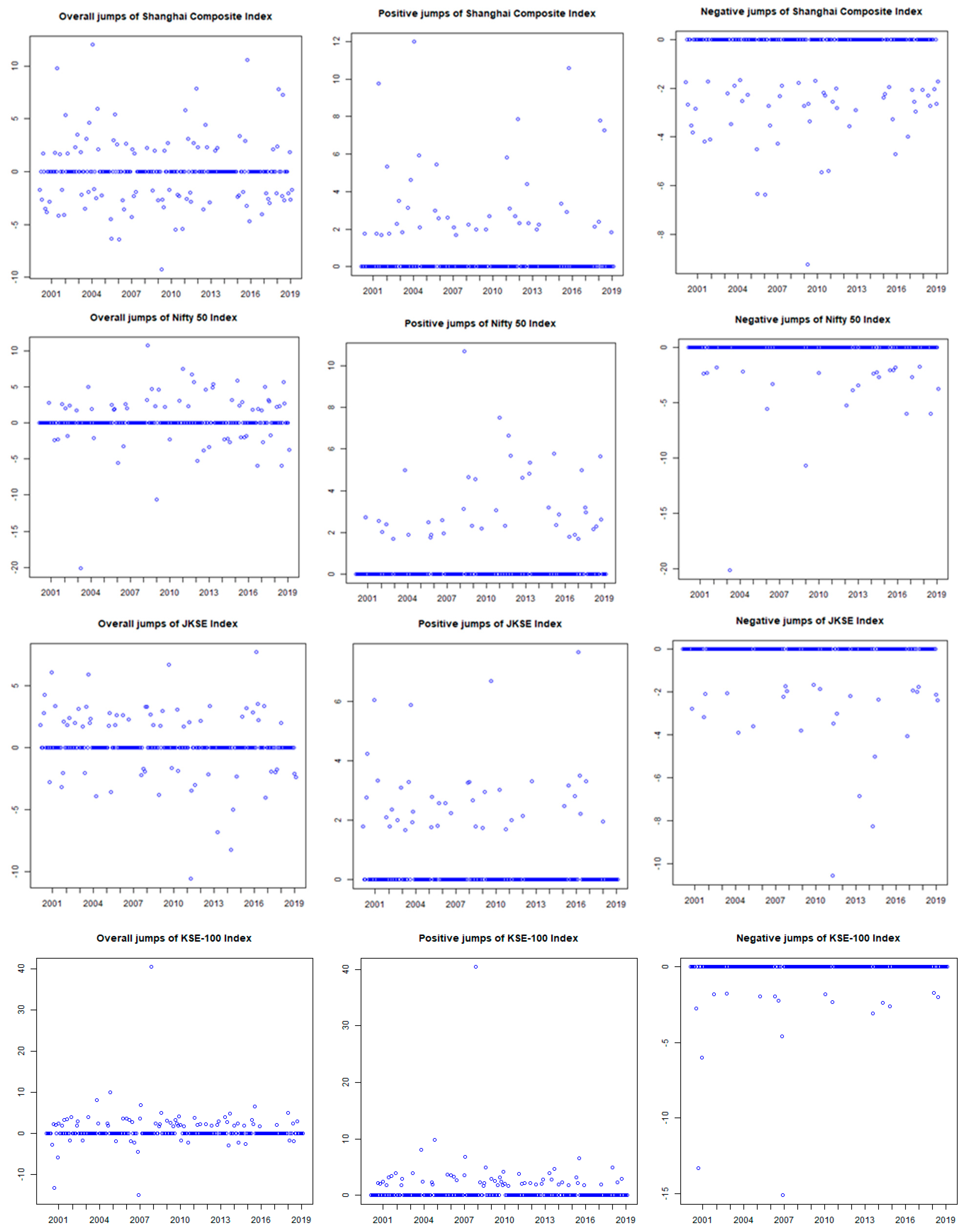
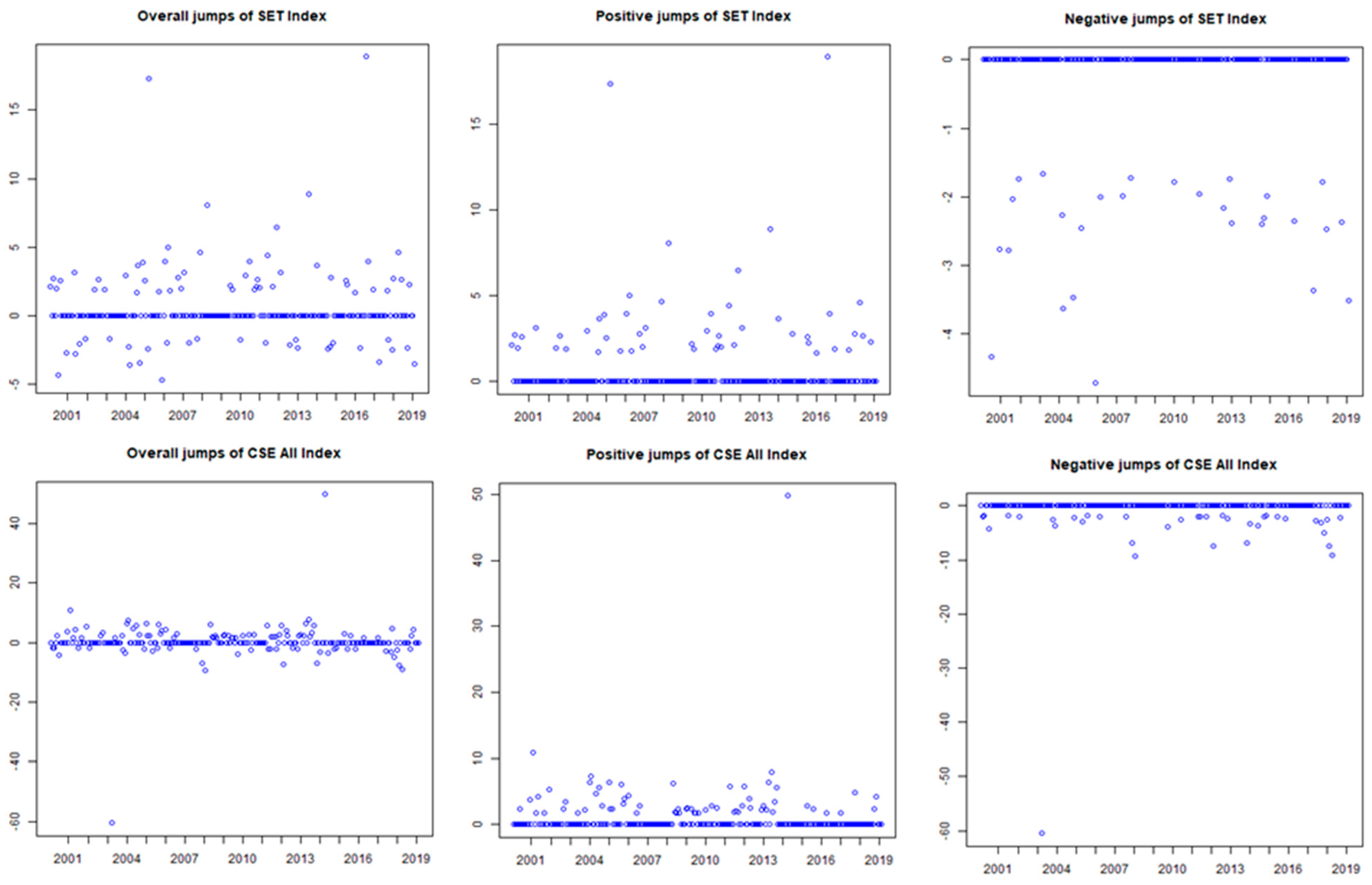
The number of months with jumps, as identified in
Table 1, is exhibited in the scatter plot (
Figure 1), showing the total number of jumps, positive jumps, and negative jumps for all equity markets in the sample period from February 2001 to February 2020. It is reflected in
Table 1 that the magnitude of some jumps is big whereas small for others. We set a cutoff point of +3 standard deviation and −3 standard deviation to distinguish small or average size jumps from big jumps. A jump with a magnitude greater than +3 standard deviation is considered a big positive jump. A jump with a magnitude between zero and +3 is considered a positive small or average size jump. Similarly, a jump with a magnitude less than −3 standard deviation is considered a big negative jump. A jump with a magnitude between zero and −3 is considered a negative average size or small jump.
It is observed from
Figure 1 that in the context of developed markets, on average, the magnitude of big negative jumps is larger than the magnitude of big positive jumps. The same pattern is also observed for emerging markets as well. However, this pattern is much higher in emerging markets as compared with developed markets.
When considering small size jumps, we do not observe much of a difference in the magnitude of negative and positive jumps in the context of developed markets. However, on average, the magnitude of small negative jumps is slightly on the higher side of the small positive jumps in emerging markets.
This means that investors considered negative information more deeply than positive information. However, the depth of feeling is on the higher side in emerging markets. It may be due to the lack of confidence of investors in the information that may cause overreaction to negative information.
Table 2 presents descriptive statistics of continuous returns (r), returns during jump periods (Jr), returns during positive jump periods (Pjr), and returns during negative jump periods (Njr) for all of the equity markets.
Table 2 shows in developed markets, the NZX50 has earned higher continuous returns per month with minimum spread indicated by standard deviation, minimum, and maximum values followed by the S&P ASX 200, so these markets are the most attractive for risk-averse investors. In comparison, the Nikkei225 has the lowest monthly continuous returns, followed by the Hang Seng with maximum spread indicated by standard deviation, minimum, and maximum values. Therefore, these markets are more volatile. For average returns during jump periods and average returns during positive jump periods, the Hang Seng and the Nikkei225 have the highest average returns per month, with maximum spread shown by standard deviation, minimum, and maximum values. Therefore, these markets are the most attractive markets for risk-taking investors. Whereas the NZX50 and the S&P ASX 200 have the lowest returns during jump periods and lowest returns during positive jump periods with maximum spread indicated by standard deviation, minimum, and maximum values. It is observed from
Table 2 that more volatile markets tend to earn larger jumps-based returns relative to less volatile markets. Furthermore, returns during positive jump periods are higher for a more volatile market than less volatile markets. Therefore, forecasting positive jumps plays an essential role for investors to earn larger returns. However, returns of more volatile markets like the Hang Seng and Nikkei225 are also more affected during negative jump periods relative to less volatile markets like the NZX50 and S&P ASX. It is worth noting that among volatile markets, a market having low returns is much more vulnerable to negative jumps.
In emerging markets, the KSE-100, Shanghai composite, and SET index are more volatile markets (as measured by the standard deviation of continuous returns) relative to others. The Shanghai Composite has the lowest continuous return, and the KSE-100 has the largest continuous return per month. In emerging markets, returns during jump periods behave differently as compared with developed markets. In the context of emerging markets, a market with average volatility and average continuous return earns the highest return during positive jump periods. Its returns are the least vulnerable during negative jump periods, i.e., the Nifty50 index. However, highly volatile markets tend to earn high returns during positive jump periods, i.e., the Shanghai Composite and KSE-100. However, highly volatile markets with high continuous returns are less vulnerable to negative jumps, i.e., the KSE-100. In contrast, highly volatile markets with the lowest continuous returns are highly vulnerable to negative jumps, i.e., the Shanghai composite.
The results of
Table 2 provide important insights to the investors in developed and emerging markets to earn the highest returns during jump periods. Investors can earn the highest returns during jump periods by investing in more volatile markets in developed markets. Investors in emerging markets can earn the highest returns during jump periods by investing in averagely volatile markets.
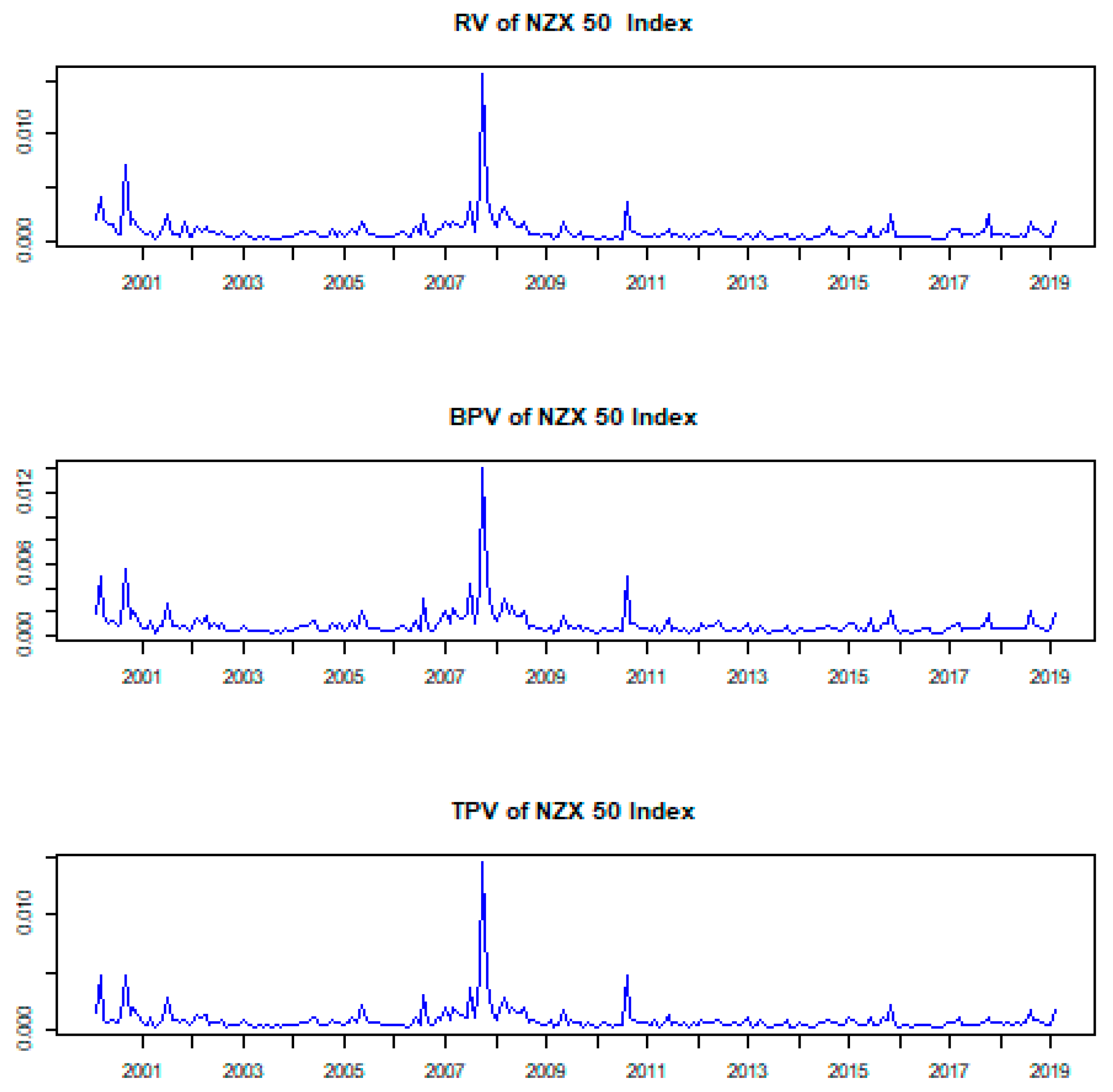
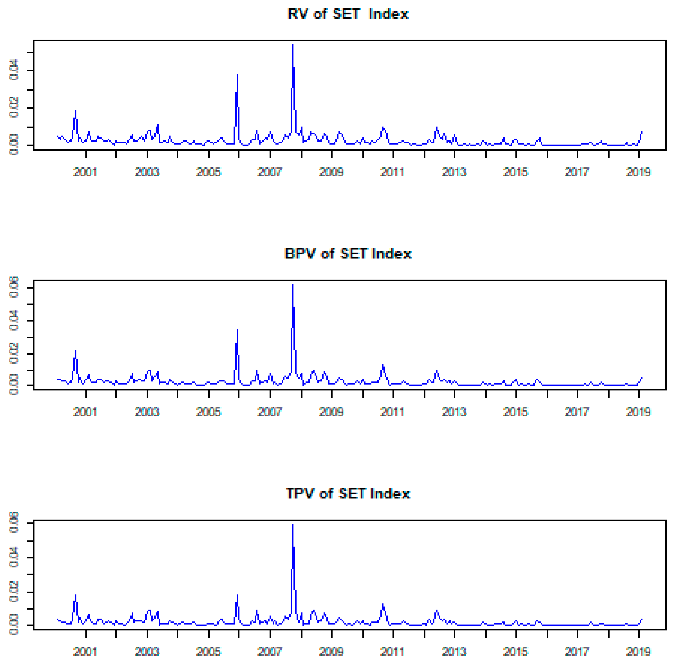
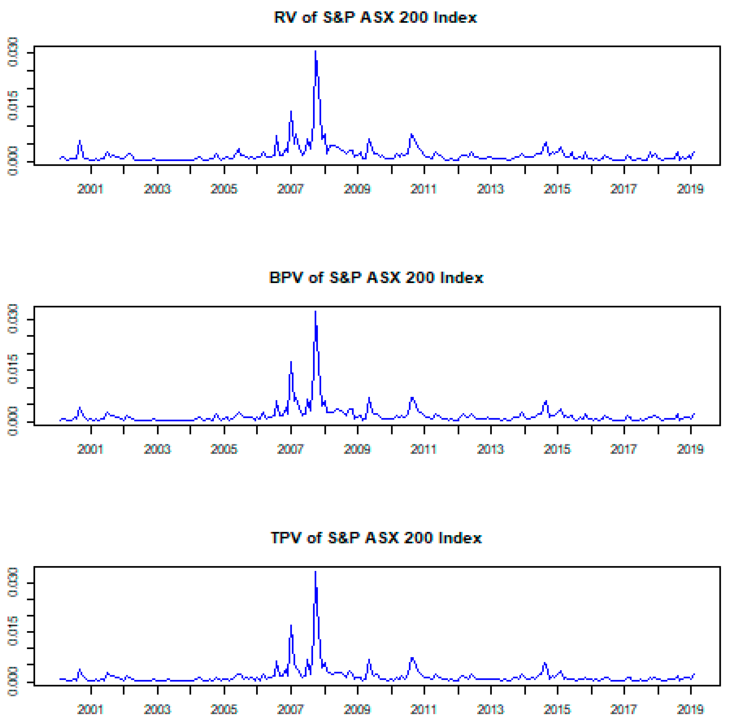
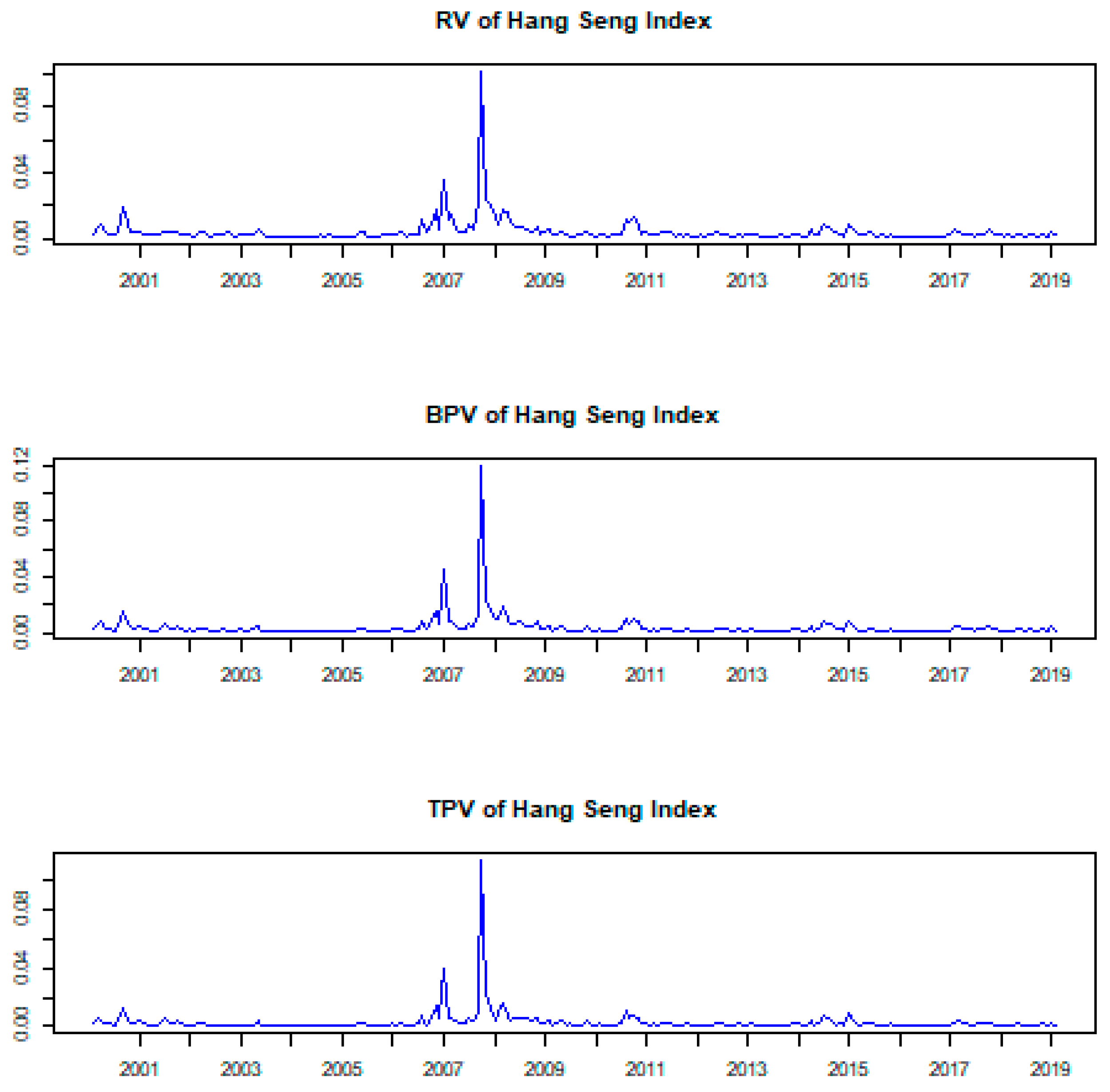
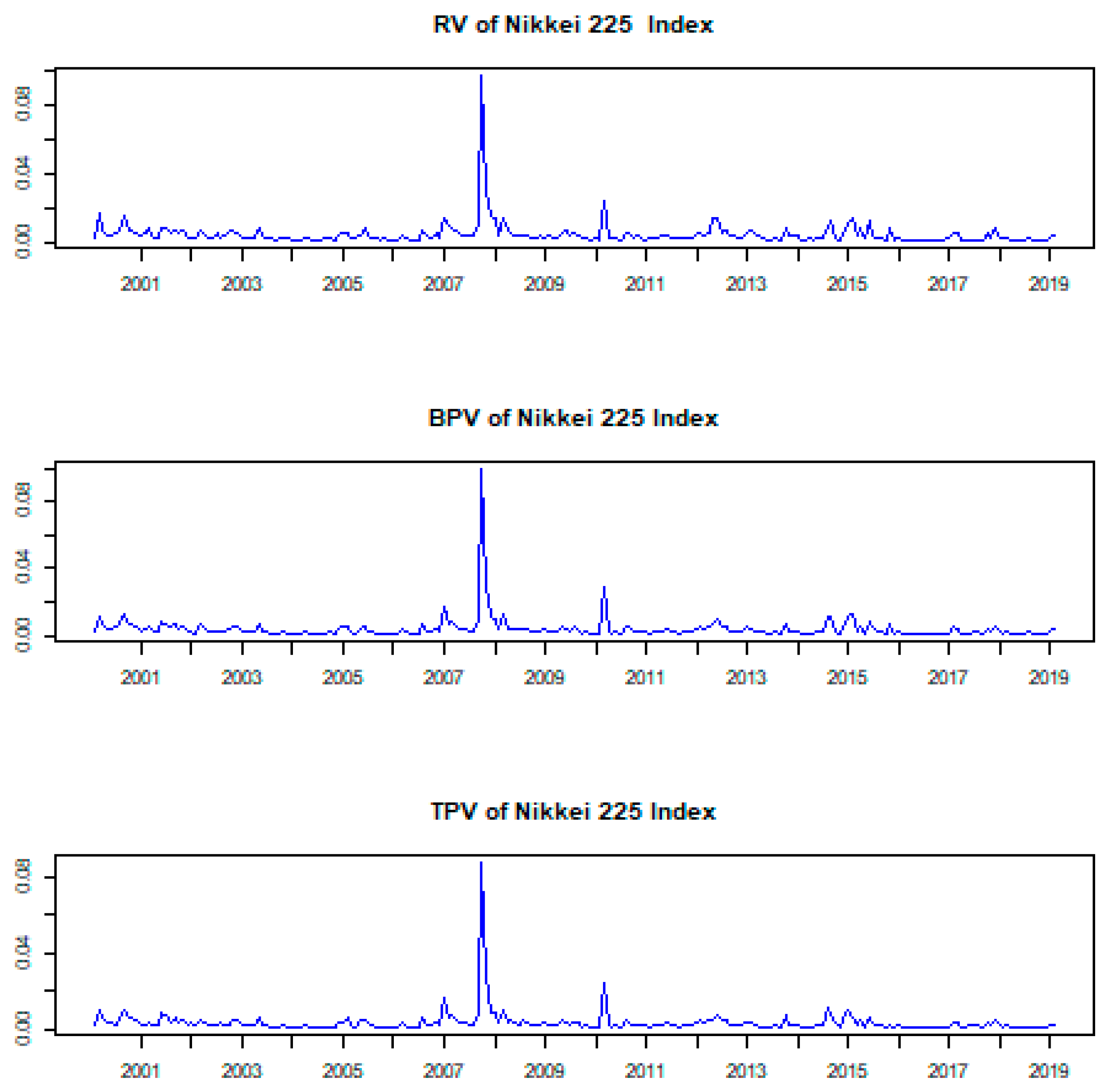
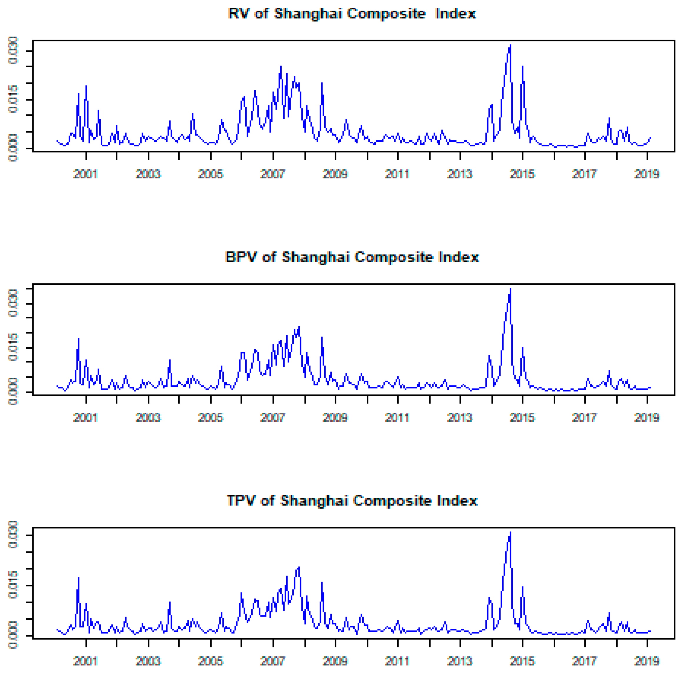
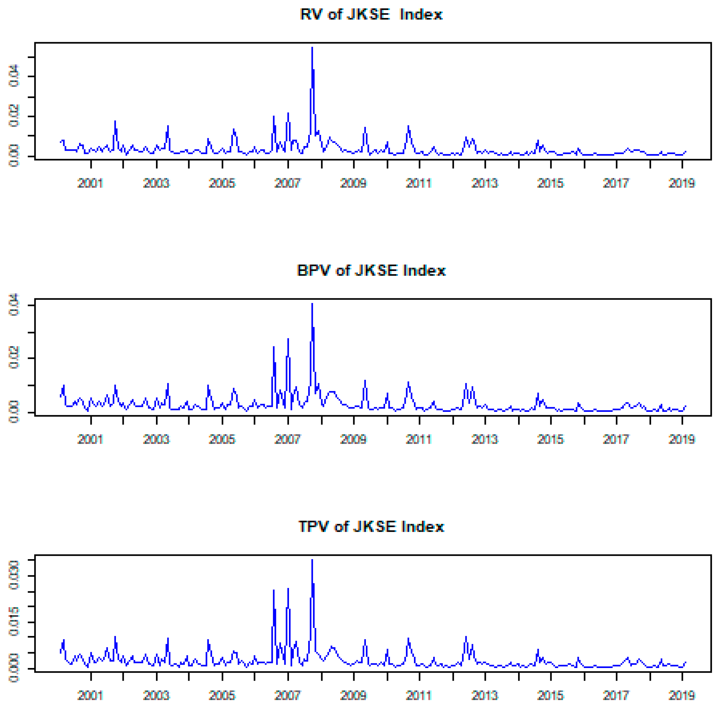
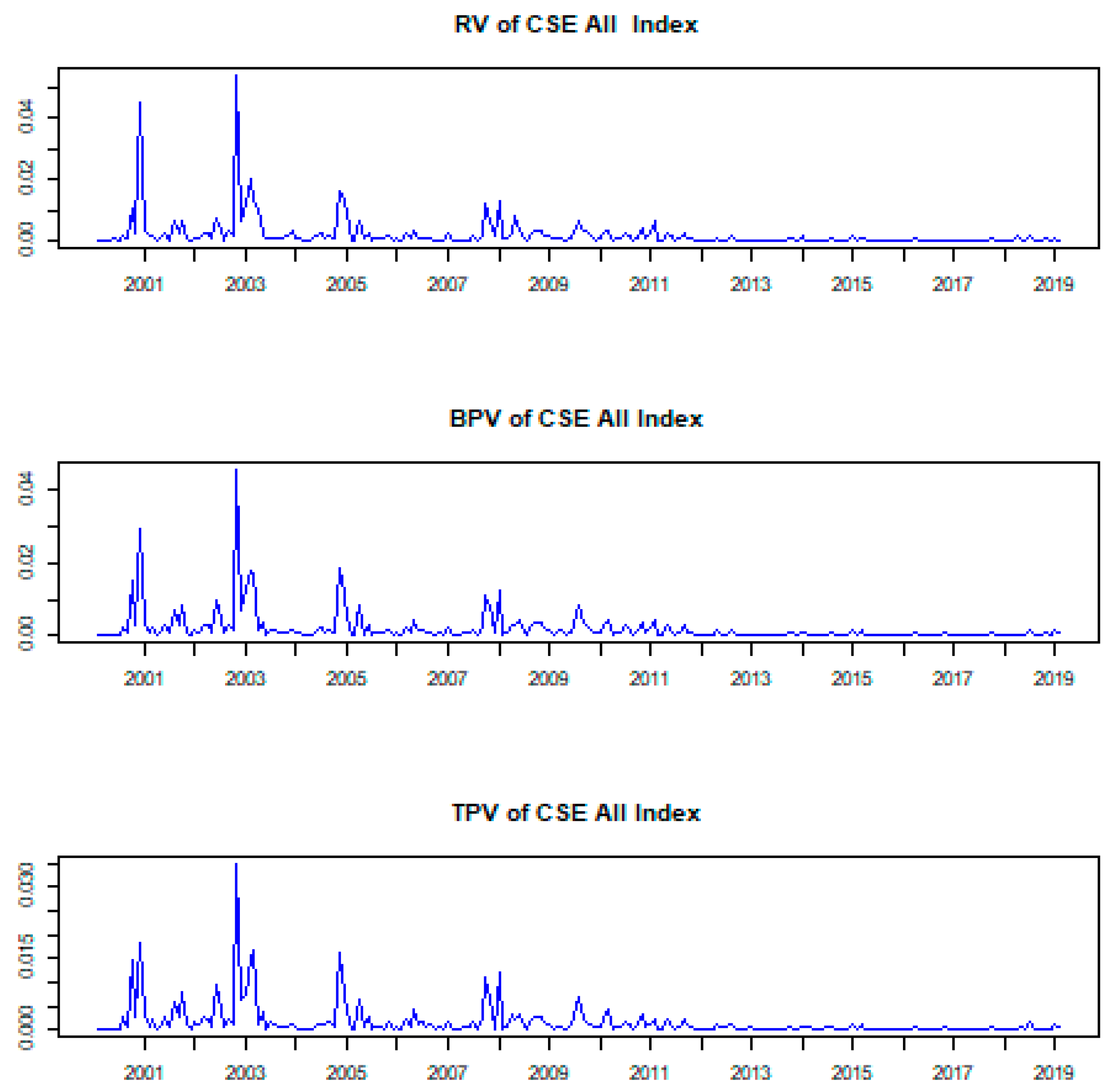
Table 3 summarizes integrated volatility, estimated using three volatility measures RV (measures total volatility), BPV (measures continuous component of quadratic variation), and TPV (also measures continuous component of quadratic variation). The mean, standard deviation, minimum and maximum values are all in terms of 10
−3. It is observed from
Table 3 that in terms of total realized volatility, the Nikkei225 and Hang Seng are more volatile markets among the developed market. Whereas among emerging markets, the Shanghai Composite shows maximum price fluctuations because it shows the highest average values of total integrated volatility. The SET index is the least volatile as its mean value of total integrated volatility is the lowest among all emerging markets. On average, emerging markets show higher integrated volatility than developed markets.
TPV is a better estimation technique of continuous components of quadratic variation than BPV as it understates the average integrated volatility and has the minimum standard deviation. This pattern is consistent across all markets. So jump-based volatility can be better estimated by the difference between RV and TPV.
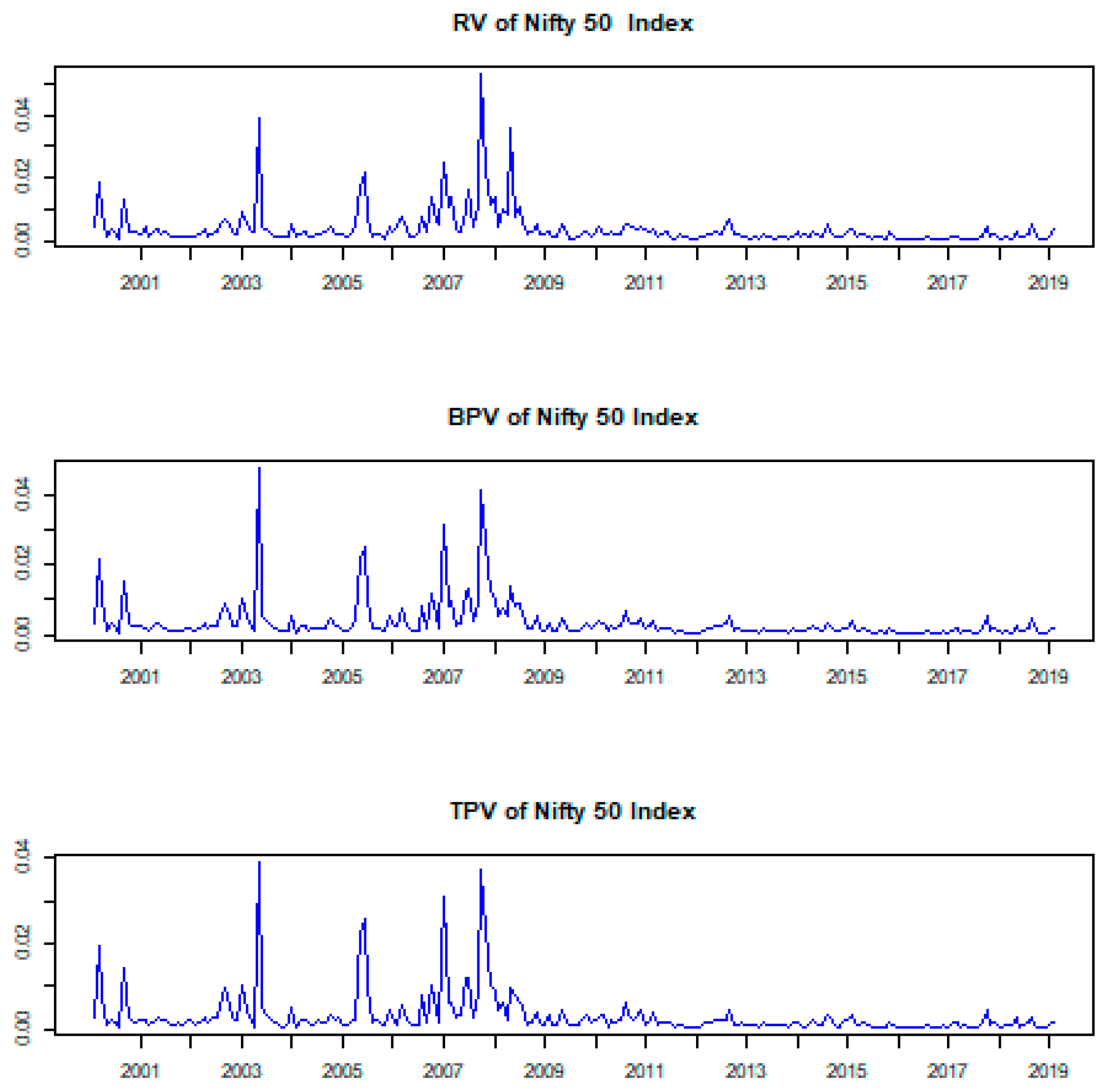
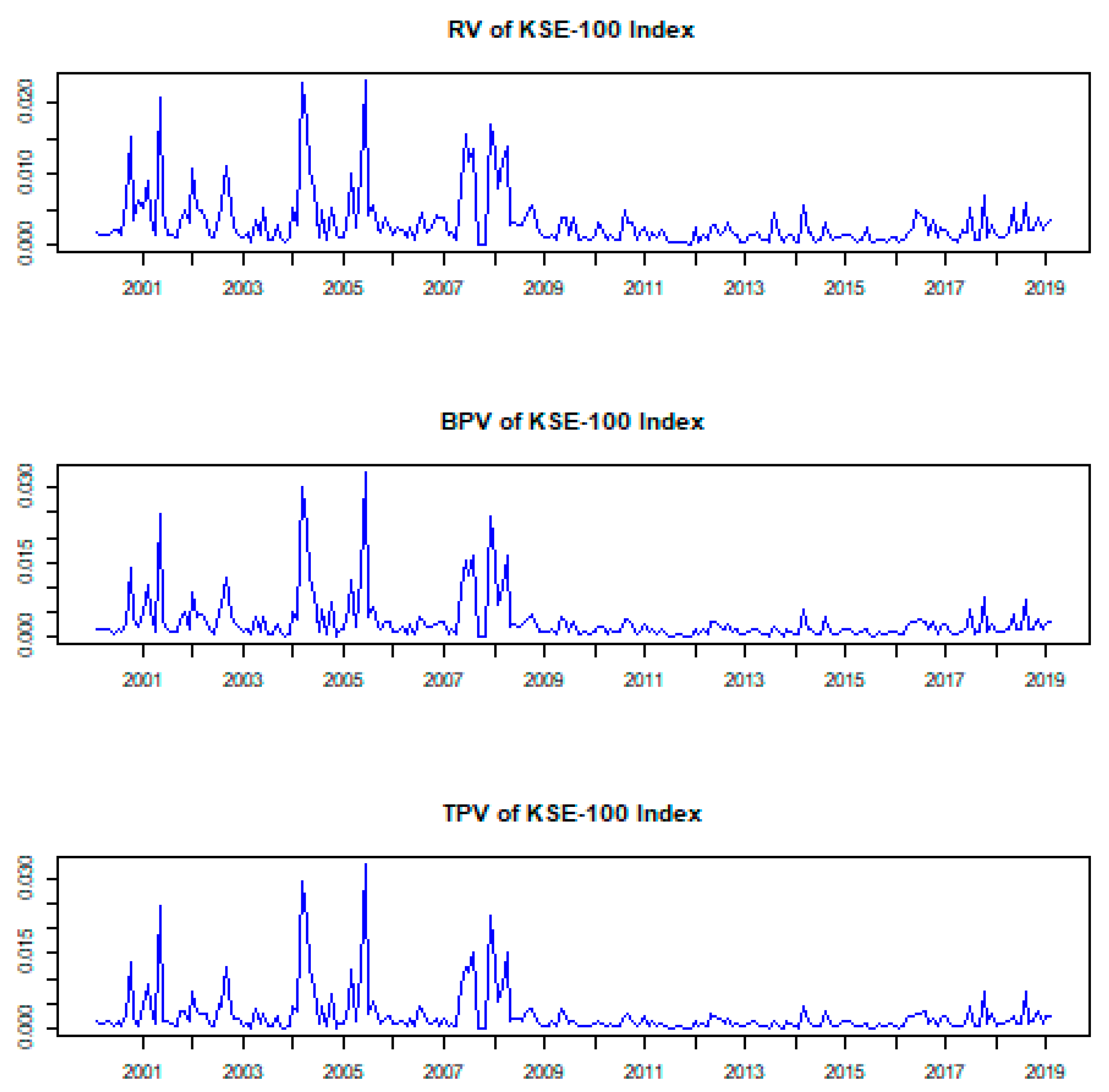
To get a clearer idea of how volatility differs across the stock markets, we turn to
Figure 2,
Figure 3,
Figure 4,
Figure 5,
Figure 6,
Figure 7,
Figure 8,
Figure 9,
Figure 10 and
Figure 11. They show the integrated volatility of the stock markets. It is noted that all individual stock markets have volatility during the financial crisis. Most of the stock markets also had their highest volatility in the 2008 crisis period. This is also in line with earlier discussion on jumps identification; in
Figure 1, it can be observed that most of the jumps have occurred during crisis periods.
For the S&P ASX 200 (
Figure 2), Hang Seng (
Figure 3), Nikkei225 (
Figure 4), NZX 50 (
Figure 5), JKSE (
Figure 8, and SET Index (
Figure 10), there seems to be little difference in terms of estimated volatility across the different volatility measures. However, in the Shanghai Composite (
Figure 6), the highest volatility was in the 2015 period, a crisis period in China; however, a similar pattern is also observed during 2008. For the Nifty50 index (
Figure 7), the peak was during 2008, but few spikes were recorded in 2003. The KSE-100 (
Figure 9) index is somewhat different from all others, which had major spikes in 2003, 2005, 2006, 2008, and at the beginning of 2009; all these periods were crisis periods in Pakistan. However, the CSE index (
Figure 11) had major spikes during 2008 for all volatility measures.
Table 4 shows the monthly volatility during jump periods for selected equity markets. First, volatility is estimated based on significant jumps. The volatility of positive and negative jumps is separated from total realized volatility.
In developed markets, the jump component shows a considerable amount of volatility in total realized volatility for all markets. However, volatility in negative jumps is higher than volatility in all jumps and volatility in positive jumps in developed markets except for with the Hang Seng, where volatility in positive jumps is higher than volatility in negative jumps. This pattern of high volatility for negative jumps is also consistent across emerging markets except the Nifty50 and CSE All index, where volatility in positive jumps is higher than in negative jumps. However, on average, total realized volatility and jumps-based volatility are larger for emerging markets than developed markets.
Table 5 shows the ratio of jump variations to total variations. The highest ratio is found in the Shanghai Composite Index. The minimum overall ratio is found for the S&P ASX 200 index. The ratio of positive jump variation to total variation is maximum for the Hang Seng index and minimum for the S&P ASX 200 index. The ratio of positive variation due to negative jump to total variation is maximum for the Nifty50 index and minimum for the NZX 50. When comparing developed and emerging markets, on average the ratio of jump variations to total variations is higher in emerging markets, Similarly, the ratio of variation during negative jump periods to total variation is also higher for emerging markets. It is concluded from the analysis that integrated volatility during a negative jump period is higher than integrated volatility during a positive jump period in both developed and emerging markets but this pattern is more pronounced in emerging markets.
7. Concluding Remarks
The purpose of this study is to examine whether jumps matter in equity market returns and integrated volatility. To accomplish the goal, we first determined jumps in market returns for both developed and emerging equity markets in Asia, including the S&P ASX 200, Hang Seng, Nikkei225, NZX 50, Shanghai Composite, Nifty50, JKSE, KSE-100, SET Index, and CSE All and disentangled the identified jumps into positive and negative jumps. We then computed both monthly average return and integrated realized volatility and compared them with monthly average returns and integrated realized volatility during positive and negative jump periods.
This paper uses the concept in an efficient capital market theory (
Fama 1970) that security prices fully reflect all relevant information and bring stock markets towards efficiency and leave no room for investors to earn excess returns. However, sometimes there exist abnormal movements or large discontinuous changes in stock prices that are infrequent but large. These extreme movements are known as jumps associated with the arrival of unexpected new information (
Ferriani and Zoi 2020;
Jiang and Zhu 2017;
Sun and Gao 2020). Jumps capture all types of information, regardless of whether it is public or private information, including insider trading. Since risk-averse investors prefer positive jumps over negative jumps as positive jumps raise stock prices, stocks with more negative jumps should receive a higher premium than those with more positive jumps (
Amaya and Vasquez 2011).
We then used the swap variance (SwV) approach developed by
Jiang and Oomen (
2008) to identify monthly jumps in the equity prices from both developed and emerging markets from February 2001 to February 2020. Further, the method developed by
Andersen et al. (
2007) was used to separate the volatility of the jump component from the total realized volatility.
Our analysis shows that jumps matter in both equity market returns and integrated volatility. We find that jumps arise in all equity markets; however, developed markets have fewer jumps relative to emerging markets. Furthermore, in all markets, positive jumps occur more frequently than negative jumps. Moreover, the magnitude of negative jumps is larger than that of positive jumps in both big and small jumps categories in emerging markets. However, the magnitude of negative jumps is larger than positive jumps only in the big jumps category for the developed market.
When average monthly continuous returns are compared with average monthly returns during jump periods, we observe that average monthly returns are higher than continuous returns during jump periods. In emerging markets, the market with average volatility earns higher returns during jump periods, whereas highly volatile markets earn higher returns during jump periods in developed markets. Moreover, markets having lower continuous returns with higher volatility are more adversely affected during negative jump periods.
Furthermore, this study reveals that realized volatility consists of a significant portion of jumps-based volatility. Integrated volatility is high during periods of negative jumps compared with periods during positive jumps. This pattern is consistent in both developed and emerging markets. The average ratio of jump variations to total variation also shows considerable variations due to jumps, indicating total realized variation consisting of substantial variations due to jumps.
Our findings infer that emerging markets are not as efficient as developed markets, and thus, jumps occur more frequently in emerging markets. Investors in all markets prefer to get positive jumps to negative jumps so that stocks with more negative jumps should have a jump risk premium. Our findings also infer that investors should avoid markets with lower continuous returns and higher volatility due to adverse effects during negative jump periods. Investors in emerging markets perceive more serious negative information than in developed markets because integrated volatility is high during negative jumps compared with periods during positive jumps, and this pattern is more pronounced in emerging markets.
The implication of this study is for all types of investors for both developed and emerging markets. The findings in our study suggest individual investors and portfolio managers of developed emerging markets avoid investment in assets and markets that are too volatile and have lower returns because these assets and markets are adversely affected by negative jumps. However, this study encourages investors and portfolio managers to invest in highly volatile assets with positive jumps because it will enable investors to earn higher returns. Furthermore, for investors in developing markets, investment in the averagely volatile assets and markets is the most efficient investment during the positive jumps period. The implication is also very important for asset pricing theory as investors prefer positive jumps to negative jumps. Therefore, stocks with negative jumps should earn a premium compared to stocks with positive jumps. This is also an important factor in the consideration of investment. This study provides insights to academics, practitioners, and policymakers on the asymmetric effect of jumps in equity market returns and integrated volatility in the context of developed and emerging markets.
One of the limitations of our study is that our data have not covered the COVID-19 period and our study is limited to Asian developed and emerging equity markets. Thus, future researchers could extend our study to cover the COVID-19 period and by including other markets in their study. Moreover, future research could consider using other techniques to estimate jumps, for example, the jump identification methods developed by
Aït-Sahalia and Jacod (
2009),
Barndorff-Nielsen and Shephard (
2006), and
Lee and Mykland (
2008). Most importantly, future studies could also incorporate jumps as a factor in asset pricing models.


