
Formulating the Concept of an Investment Strategy Adaptable to Changes in the Market Situation


1
Department of Data Analysis and Machine Learning, Financial University under the Government of the Russian Federation, 125993 Moscow, Russia
2
Department of Higher Mathematics, Bauman Moscow State Technical University, 105005 Moscow, Russia
Economies 2021, 9(3), 95; https://0-doi-org.brum.beds.ac.uk/10.3390/economies9030095
Submission received: 8 May 2021
/
Revised: 12 June 2021
/
Accepted: 16 June 2021
/
Published: 23 June 2021
Abstract
:The study aims to develop a dynamic model for the management of a strategic investment portfolio, taking into account the impact of crisis processes on asset value. A mathematical model of a dynamic portfolio strategy is developed, and guidelines for framing a long-term investment strategy based on the current state of the investment market are formalized. An efficient method of long-term ensemble forecasting to increase the accuracy of predicting financial time series is elaborated. A methodology for constructing and rebalancing a dynamic strategic investment portfolio based on a changing portfolio strategy that results from assessing the current market state and forecast is developed. The obtained strategic portfolio model has been estimated empirically based on historical data and its rate-of-return characteristics have been compared with those of the existing conventional models used in strategic investment.
1. Introduction
Choosing the right investment mechanism is one of the main tasks for any investor, requiring careful analysis and research of all available information (Yerznkyan et al. 2021). Therefore, no investor knows exactly whether their expectations regarding the return on particular equity will be met, but they need to build their strategy in such a way as to eliminate the damage as much as possible in the event of an unfavorable outcome. The development of a universal investment vehicle could facilitate the activities of investors; however, it seems a challenging task thus far to build a unified model that covers the whole variety of factors. Creating an investment portfolio is an urgent issue in the current conditions of the rapid evolution of the stock market and is growing interest in investment from all participants in the economy.
The securities portfolio acts as an integral object of management. To solve the problem of the optimal securities portfolio means determining the optimal allocation of the asset shares in the portfolio, such that it meets the investor’s goals. In 1952, in The Journal of Finance, Harry Max Markowitz, Professor of the University of Chicago, published his work, “Portfolio Selection” (Markowitz 1952), from which the theory of portfolio investment originates. In the article, H. Markowitz suggests a mathematical model for forming an optimal portfolio of securities.
A foundational step in the development of portfolio analysis was made by R. Roll. He developed a regression method for investment portfolio optimization known as Roll’s rebalancing (Roll 1977). The ratio between the geometric and arithmetic mean rates of any set of the return components is used as a portfolio return indicator. In this case, all the components being equal, a rebalanced portfolio always outperforms an unbalanced one.
A substantial contribution to the study of portfolio strategy, dynamics and optimization of the investment portfolio was made by Dai Pra, P., andTolotti, M. (Dai Pra and Tolotti 2009). The authors provided mathematical proof that a set of asset groups is more stable than each asset individually.
The authors Li, B., Sun, Y., Aw, G., and Teo, K. L. (Li et al. 2019) suggest using the Pareto equilibrium point to find the optimal static portfolio in a steadily growing market. The mathematical model is fully justified but has not been tested in practice. The authors argue that under certain conditions, such a portfolio may perform better than the minimum-risk portfolio by H. Markowitz.
The authors de Leeuw, T., Gilsing, V., and Duysters, G. (de Leeuw et al. 2019) compare a static, state-regulated portfolio model and five diverse, dynamic portfolio models with different dynamicity levels and find that despite a more than twofold difference in return demonstrated by dynamic models, a dynamic portfolio is preferable to a static portfolio which is recommended or regulated by the state.
The authors Bi, J., and Cai, J. (Bi and Cai 2019) recommend using an equilibrium portfolio strategy with constraints, and proposed to introduce the upper and lower VaR control limits that determine the need to change the equilibrium point of the portfolio strategy.
The authors Hadhri, S., and Ftiti, Z. (Hadhri and Ftiti 2019) suggest that for portfolio optimization, the measure of skewness should be used as a criterion, along with the classical risk/return pair. The authors note that for a static portfolio, skewness is an important element that characterizes asset instability.
The authors Jeon, J., and Shin, Y. H. (Jeon and Shin 2019) address the choice of strategy in marginal markets under a finite investment horizon and offer a mathematically sound model of gradient optimization, which allows achieving minimal risk with minimal loss of a static portfolio.
The authors Wei, J., Bu, B., and Liang, L. (Wei et al. 2012) propose the simplest two-mode dynamic portfolio model that has a high-risk and low-risk mode and switches the strategy depending on arbitrarily determined external risk factors.
The authors Benita, F., López-Ramos, F., and Nasini, S. (Benita et al. 2019) present a four-level dynamic portfolio model that switches the strategy used depending on arbitrarily determined external risk factors.
The study (Lu et al. 2020) aims to use both the Sharpe ratio (SR) and the economic performance measure (EPM) to compare the performance of DCA and LS under both accumulative and disaccumulative approaches when the asset price is simulated to be in an uptrend.
The literature review has shown that the best investment strategy is one that adapts to external factors.
The authors Ma, G., Siu, C. C., and Zhu, S. P. (Ma et al. 2019) propose a dynamic portfolio that is optimized based on the analysis of the predicted market situation, instead of relying on the current trends. In fact, the authors recommend using the classic Merton portfolio, optimized based on the expected market conditions. The authors Lu, Y. N. et al. (Lu et al. 2018) suggest splitting the investment portfolio into several different portfolios with different strategies. In doing so, the method of strategic diversification is implemented. In fact, in this paper, the authors described a new method of portfolio diversification, namely, strategic diversification. Golosnoy, V., Gribisch, B., Seifert, M. I. (Golosnoy et al. 2019) suggest predicting the portfolio behavior by obtaining separate predictions for each asset share in the portfolio. Empirical evidence shows that the combined forecast of the asset shares is more accurate in practice than the forecast made for the entire portfolio.
In the above studies dedicated to the analysis of portfolio investment, almost no attention is paid to the specification of the strategy, nor to methods of scoring its performance, or to the adaptability of strategies. To date, the only traditionally used method of scoring a strategy’s performance is simulation modeling.
Having formalized the components of an investment strategy, one can develop and apply quantitative methods of strategy evaluation.
In this regard, the scope of the in-depth scientific study was defined as follows: 1. observation of the methods of system analysis; 2. formalization of the construction and evaluation of investment strategies; 3. synthesis of various approaches based on the refinement of classical and neoclassical theories, as well as the creation of models and methods of strategic investment taking into account the real state of the market with an allowance for the risk of crisis changes.
2. Literature Review
To date, many works have been concerned with the creation of investment portfolios using innovative mathematical tools of machine learning and fuzzy logic. Let us look at some of them.
In the work of Chen Shun and Ge Lei (Chen and Lei 2021), the strategy of an optimal investment portfolio selection based on a neural network model is investigated. A numerical comparison of the results obtained in the article with those of classic solutions demonstrates the effectiveness of the learning-based strategy. To select the optimal portfolio, in the work of Zhou Wei and Zeshui Xu (Zhou and Xu 2018), qualitative models for portfolio construction under uncertain conditions of a fuzzy environment were proposed. Guan Hao and Zhiyong An (Guan and Zhiyong 2019) propose a local adaptive learning system for selecting an online portfolio. In their article, Park, Hyungjun, Min Kyu Sim, and Dong Gu Choi (Park et al. 2020) suggest a novel portfolio-trading strategy in which an intelligent agent is trained to identify an optimal trading action by using deep Q-learning. In their study, Ma Yilin, Ruizhu Han, and Weizhong Wang (Ma et al. 2021) suggest optimizing the portfolio based on the prediction of asset returns. The authors use five models for predicting stock returns, which improves the quality of stock selection for constructing an investment portfolio. Francesco Cesarone, Carlo Mottura, Jacopo M Ricci, and Fabio Tardella (Cesarone et al. 2020) compared several popular investment portfolio selection models in terms of their sensitivity to noise. The results showed that the portfolios with the highest returns are the most sensitive to noise. Felipe Dias Paiva, Rodrigo Tomás Nogueira Cardoso, Gustavo Peixoto Hanaoka, and Wendel Moreira Duarte (Paiva et al. 2019) propose a decision-making model for day-trading investments on the stock market. The model is based on the support vector machine method and the mean-variance method for portfolio selection. In the work of Khedmati Majid and Pejman Azin (Khedmati and Azin 2020), an online portfolio-selection algorithm based on the pattern-matching principle is presented. In their work, Eom Cheoljun and Jong Won Park (Eom and Park 2019) developed a method for estimating a correlation matrix, on the basis of which a well-diversified portfolio was constructed. In their article, Jinhua Chang, Lin Sun, Bo Zhang, and Jin Peng (Chang et al. 2020) consider the uncertain multi-period portfolio selection problem in a situation where future security return rates are given by experts’ estimations instead of historical data. The paper provides a case study that illustrates the effectiveness of the developed model. Xiaomin Gong, Changrui Yu, Liangyu Min, and Zhipeng Ge (Gong et al. 2021) propose a model for evaluating cross-efficiency scores of assets aimed at maximizing an investor’s perceived utility (composed of utility, regret, and rejoice functions). To demonstrate the effectiveness of the proposed model, a real-world empirical application is presented. Xingying Yu, Yang Shen, Xiang Li, and Kun Fan (Yu et al. 2020) consider the mean-variance portfolio selection problem with uncertain model parameters. The authors formulate the mean-variance problem under the maxmin criterion. Using the Lagrangian method, an efficient portfolio is obtained. In their article, Puerto Justo, Moisés Rodríguez-Madrena, and Andrea Scozzari (Puerto et al. 2020) propose a linear programming approach to solve the portfolio-selection problem. When almost all underlying assets suddenly lose a certain part of their nominal value in a market crash, the diversification effect of portfolios under normal market conditions no longer works. Shushang Zhu, Wei Zhu, Xi Pei, and Xueting Cui (Zhu et al. 2020) assess the crash risk in portfolio management and investigate hedging techniques involving derivatives to optimize the investment portfolio. In the study by Mansour Nabil, Mohamed Sadok Cherif, and Walid Abdelfattah (Mansour et al. 2019), they developed an approach involving fuzzy parameters, where the possibility distributions are given by fuzzy numbers from the information supplied by the decision-making environment (investor, analyst, financial market environment, etc.). The proposed financial portfolio selection model with fuzzy returns is used within the stock exchange market and discussed in comparison with other portfolio selection models. Guoli Mo, Chunzhi Tan, Weiguo Zhang, and Fang Liu (Mo et al. 2019) suggest forming an international portfolio of stock indices with spatiotemporal correlation. The research by Mishra Sasmita and Sudarsan Padhy (Mishra and Padhy 2019) proposes an efficient investment portfolio construction model using predictive analytics based on support vector regression. Gang Chu, Wei Zhang, Guofeng Sun, and Xiaotao Zhang (Chu et al. 2019) propose a new online portfolio selection algorithm based on the Kalman filter and anticorrelation. In the article by Borovička, Adam (Borovička 2020), a unique fuzzy multiple objective programming algorithm is proposed for creating a portfolio in conditions of uncertainty.
3. Methodology
To create an efficient modern portfolio model, we will develop a basic strategic concept. When creating the concept, we will rely on several generally accepted economic hypotheses.
Hypothesis H1:
Based on historical data and methods of multivariate regression analysis, it is possible to construct a strategic investment portfolio that will periodically change its investment strategy and break even regardless of the current market situation.
Hypothesis H2:
The market state is stable or tends to be one in which supply and demand are balanced.
Corollary to Hypothesis H2: we can break down the market state in the following terms:
- Stagnation—a stable state;
- Growth—a situation where demand exceeds supply;
- Decline—a situation where supply exceeds demand.
Hypothesis H3:
The hypothesis of the identical character of crises. The phases of economic crises are always identical.
3.1. The Concept of an Innovative Investment Strategy Adaptable to Changes in the Market Situation
To form the basic concept, we define a market as any non-empty set of traded assets. Such a system is characterized by the following conceptual approaches:
- Combined market—part of the market information is distributed instantly, is publicly available, and directly reflected in the price of the asset; the other part is reflected with a delay or indirectly (Gataullin et al. 2020; Gorodetskaya et al. 2021; Yerznkyan et al. 2019).
- Combined return—changes in the price of an asset can be considered as an aggregated stochastic process; the speculative preferences of investors (Sunchalin et al. 2019; Ivanyuk and Tsvirkun 2013).
- Segmented market—any non-empty set of assets can simultaneously be considered as a market, a portfolio, or an asset itself if the set contains a single element.
- Limited market—in market development, time constraints are determined by the forecast horizon.
- Forecasted market—in market development, most trends are predictable.
- Rational investor—the investor’s interest is to achieve the maximum possible increase in the portfolio value during the forecast period with the minimum predicted risk.
- Finite investment period—the duration of the investment period is determined by the forecast horizon.
According to the above concepts, the market states are different at different times. The differences are so great that there is no single investment strategy that would be profitable in any time period, under any market conditions. The main conceptual approach that follows from the above is that the investment strategy must be changed in accordance with market developments.
The main advantages of this concept include:
- balance between disregarding instantaneous market changes and taking into account fundamental market factors;
- adaptability of the strategy;
- predictively justified approach to the optimal portfolio creation.
Let us form a general algorithm for implementing the strategy:
- Data acquisition;
- Market analysis;
- Portfolio strategy adjustment;
- Asset selection;
- Forecasting;
- Portfolio rebalancing.
Basic strategy: change the strategy at every rebalancing event. The strategy is formed by the market (Figure 1).
The mathematical expression of this concept is the value of the optimal asset share of the portfolio, depending on the superposition of functions, as written below:
where: —a set of historical market data; —the portfolio share of the asset.
3.2. Algorithm for Developing an Innovative Investment Strategy That Is Adaptable to Changes in the Market Situation and Has the Properties of an Open System
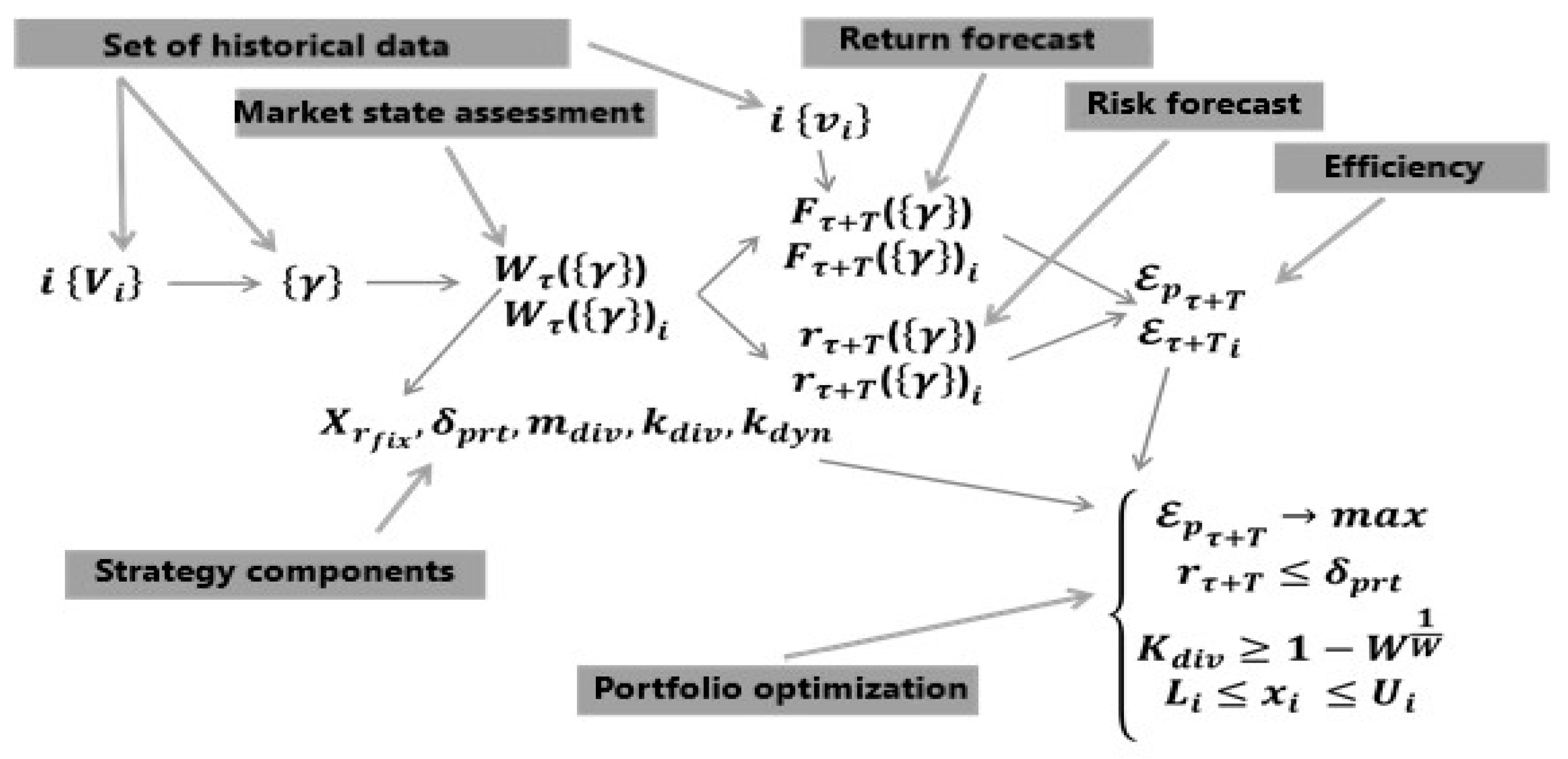
The algorithm for forming a dynamic strategy portfolio can be presented as Figure 2.
4. Methodology for the Development of an Adaptive Investment Strategy
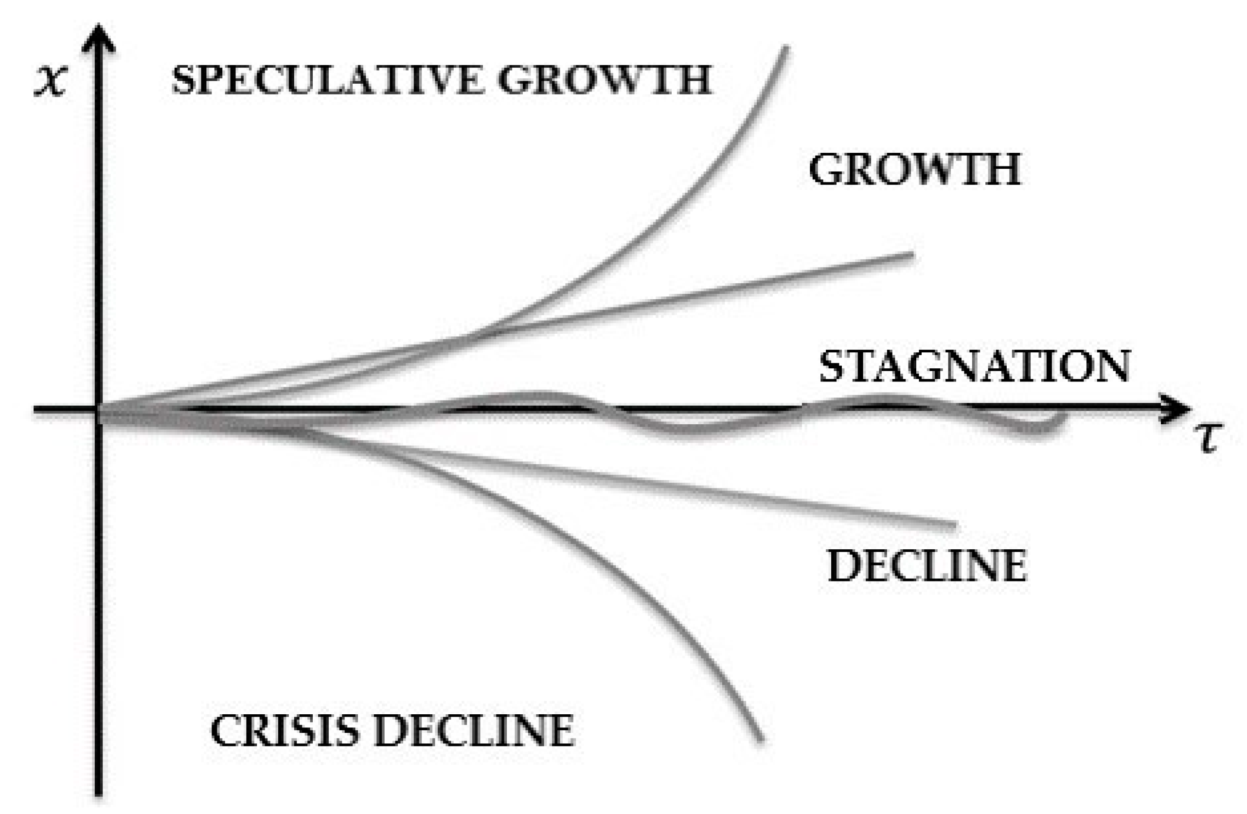
Let us define a set of possible results of the state analysis function W = Analythic({γ}) presented by the decrease of the potential profit: Speculative growth, Growth, Dynamic stagnation, Decline, Crisis decline (Figure 3).
To create an initial market assessment, we determine the boundaries of basic normalized states on the interval [0; 1], taking into account that the state of dynamic stagnation is a constant (see Table 1).
To determine the market state at the time t for the beginning of the investment period , we will use data on the market state for the preceding period .
4.1. Model of Dynamic Stagnation of the Asset Value
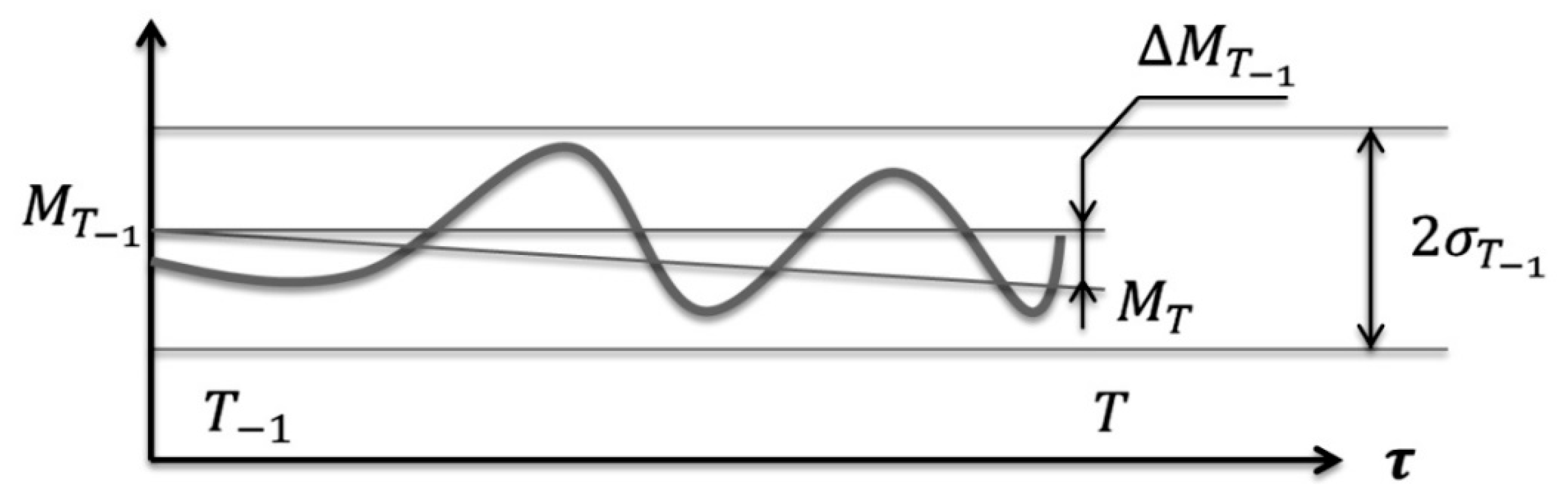
We define dynamic stagnation as a situation where the asset value lies in the price corridor of the -th probability: , provided that lies within the inflation-conditioned limits (Figure 4).
The width of the permitted movement corridor is assumed to be equal to the sum of the inflationary factor for the periods and :
Then, the state of dynamic stagnation Equation (2) is expressed as :
where: —indicator of stagnation; —Heaviside function: ; —inflationary factor; —mathematical expectation for ; —standard deviation for .
4.2. The Model of Growth and Decline of the Asset Value
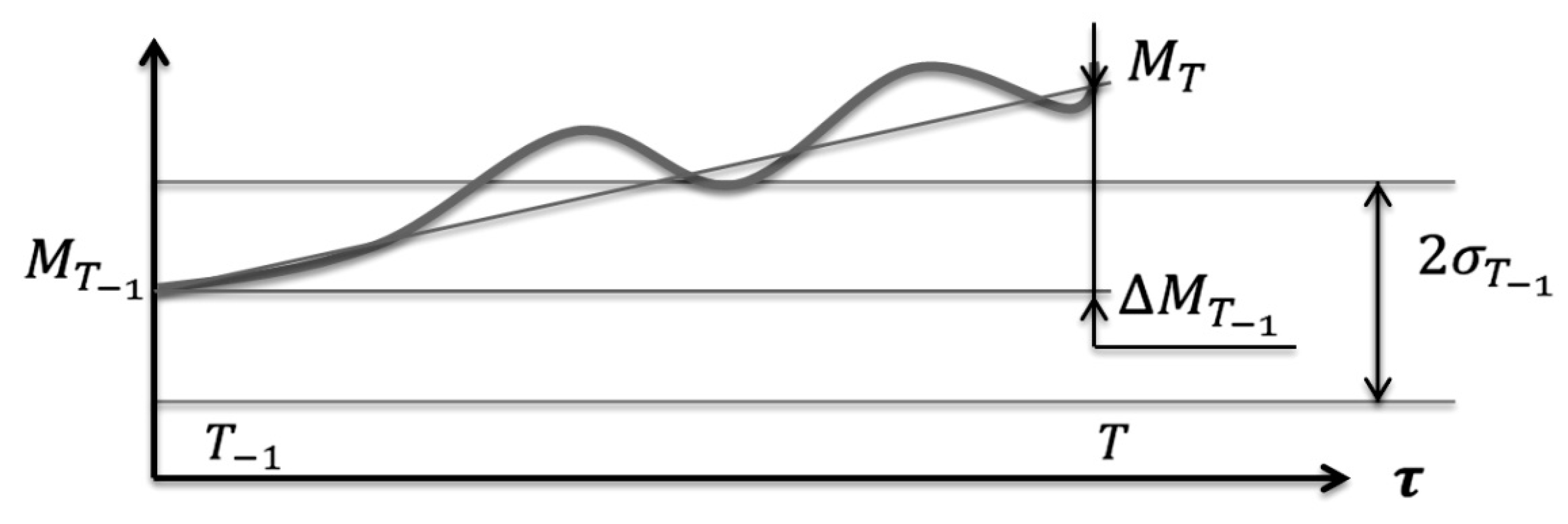
The direction of the return indicator for the investment period can be defined as the difference in the values of the mathematical expectation of the portfolio market value for the current period and the previous period : positive values indicate growth, negative values indicate a decrease (Figure 5)
Then, we will express the share of the market growth Equation (3) on the interval as:
where:
—share of market growth (decline)
—Kronecker function:
—change in the mathematical expectation for the period
—the largest change in the value for the period achieved over the entire period of the asset’s existence .
Thus, the state of a non-crisis market, in view of stagnation, can be expressed as Equation (4):
where: —non-crisis market state
4.3. Asset Crisis Model
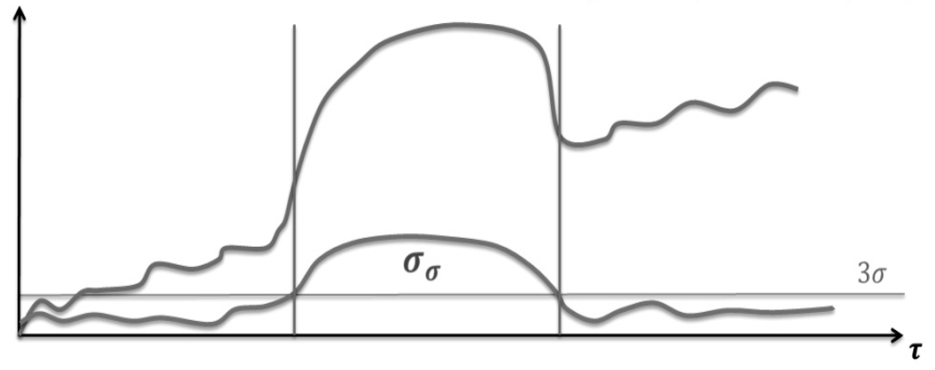
Let us define a crisis as an imbalance of positive and negative indicators that exceeds the statistically valid probability bounds set at 99.7%. Based on the three-sigma rule, all values of a normally distributed random variable lie within the interval . Let us estimate the crisis state as a situation where the volatility indicator falls outside the statistically predicted range (Figure 6):
The Figure S1 from Supplementary File shows the graph Crisis phase identification.
During the crisis period, the intrinsic deviation of volatility exceeds the threshold value of three sigmas: , where —the intrinsic standard deviation of volatility. The presence of a crisis and the direction of its development can be expressed in the interval as Equation (5):
where:
—weight coefficient of the crisis in the state function;
—change in the mathematical expectation for the period
—volatility (standard deviation) of the indicator;
—standard deviation of volatility;
—the highest ratio achieved in the entire historical period.
We will formulate a generalized analytical function of the current market state Equation (6):
where: —market state function.
4.4. Asset Investment Strategy Model
We propose a portfolio model with an adaptive strategy that is optimized with regard to the market state.
Let us imagine a market strategy model as an aggregate of constituent elements Equation (7):
where: —weight of the portfolio strategy element, —number of strategy elements, —aggregated estimate of portfolio strategy.
Let us define the most common elements of portfolio investment strategies:
- Profit-taking threshold;
- Aggregate portfolio risk;
- Type of portfolio diversification;
- Degree of portfolio diversification;
- Degree of portfolio dynamicity (rebalancing frequency).
Then, the portfolio strategy estimate can be represented as Equation (8):
where: —upper profit-taking threshold; —aggregate portfolio risk; —type of diversification; —degree of diversification; —degree of portfolio dynamicity.
Development of the strategy is dependent on the market state. For the purpose of profit maximization, the strategy must be aligned with the market condition; hence, more aggressive elements of the strategy will be optimal for growing markets, while more cautious ones—for declining markets. Let us order the components of the strategy by the aggressiveness/cautiousness ratio according to the state of the market (Table 2).
Methods of calculating the strategy elements: let us calculate the weight coefficients of the strategy components Equation (9):
where: —weight coefficient of the strategy component; —the ordinal number of the strategy element; —number of strategy elements; —the current value of the market state.
Determination of the profit-taking threshold: to reduce the risk, we will determine the upper threshold of the portfolio profit-taking Equation (10):
where: —the current value of the market state; —upper profit-taking threshold of the portfolio value; —the initial portfolio value.
Determination of the risk component of the portfolio strategy: let us define the acceptable boundaries of the risk corridor as , then the recommended portfolio risk is Equation (11):
where: —recommended portfolio risk; —risk of the most reliable asset in the portfolio; —risk of the least reliable asset in the portfolio.
Determination of the type of portfolio diversification: let us determine the type of diversification for the investment portfolio being formed: we will rank the types of diversification by the degree of risk increase (Table 3).
, then the optimal type of portfolio diversification is Equation (12):
where: —type of portfolio diversification.
Determination of the degree of portfolio diversification: let us define the boundaries of portfolio diversification as , then the recommended degree of portfolio diversification is Equation (13):
where: —the degree (coefficient) of portfolio diversification.
Determination of dynamic portfolio strategy: let us express the portfolio dynamicity as the ratio of the number of rebalancing events for the period to the maximum possible number of them, taking into account the duration of the investment period as the maximum possible value of Equation (14):
Then, the recommended of the portfolio is Equation (15):
The compliance of the portfolio strategy with the current market situation rules (strategy quality) can be estimated by Equation (16):
where: —the value of the current market state; —the value of the selected portfolio strategy element.
Table 4 shows Compliance of portfolio strategy with the current market situation.
The main task for each rebalancing of the portfolio is to determine the optimal parameters of the portfolio strategy elements for the corresponding market state Equation (17):
System of equations for the portfolio strategy: thus, the dependence of the optimal portfolio strategy elements on the market state can be expressed as (18):
where and are the elements of the strategy that affect the global characteristics of the portfolio—absolute risk and sensitivity, while , and affect the asset share allocation within the portfolio.
This optimization can be performed using the stochastic gradient descent method.
4.5. The Aggregate Forecast Model for an Asset in the Market
Time series forecasting is a matter of high value and importance, so a large number of papers are devoted to this topic. Let us review the scientific papers of contemporaries.
In the paper by Wu, Y. X., Wu, Q. B., and Zhu, J. Q. (Wu et al. 2019), the authors propose a novel model based on ensemble empirical mode decomposition (EEMD) and long short-term memory (LSTM). They obtain results that demonstrate that the hybrid approach works well even when the number of decomposition results varies.
Zhu, J., Liu, J., Wu, P., Chen, H., and Zhou, L (Zhu et al. 2019) used the ensemble empirical mode decomposition (EEMD) and optimal combined forecasting model (CFM) and obtained results that show that the proposed approach outperforms benchmark models.
Wang, M., Zhao, L., Du, R., Wang, C., Chen, L., Tian, L., and Stanley, H. E. (Wang et al. 2018) propose a novel hybrid method that uses an integrated data-fluctuation network (DFN) and several artificial intelligence (AI) algorithms, and is named the DFN-AI model. The results of their study demonstrate that the combined model performs significantly better than their corresponding single models in terms of accuracy.
Abdollahi, H. (Abdollahi 2020) proposes a novel hybrid model for crude oil price forecasting, whose focus is on improving the accuracy of prediction, taking into consideration the characteristics existing in the oil price time series. Finally, empirical results demonstrate that the proposed hybrid model outperforms other models.
The literature review has shown that the best method is the combined ensemble forecasting method. The choice of the forecasting method in the study was motivated by the fact that the ensemble forecasting method was taken as a basis.
We use an aggregate ensemble forecast to predict the value and risk of assets. We shall form such a forecast as a combination of regressions, where it should contain elements that reflect:
- Growth or decline tendencies (linear component);
- Tendencies to growth boundedness (logarithmic component);
- Seasonality and periodicity tendencies (harmonic component);
- Tendencies to the influence of prior conditions (autoregression);
- Tendencies to the influence of external factors (complex regression).
In other words, the aggregate forecast is the averaged value of the results of several regression forecasting techniques, obtained based on the confidence coefficients of the techniques in question Equation (19).
The confidence coefficient is the ratio of geometrically averaged correlation coefficients of a set of forecasts obtained by a certain technique to the sum of geometrically averaged correlation coefficients of all the forecasting techniques used Equation (20):
Let us consider the main forecasting methods that are used to form the aggregate forecast.
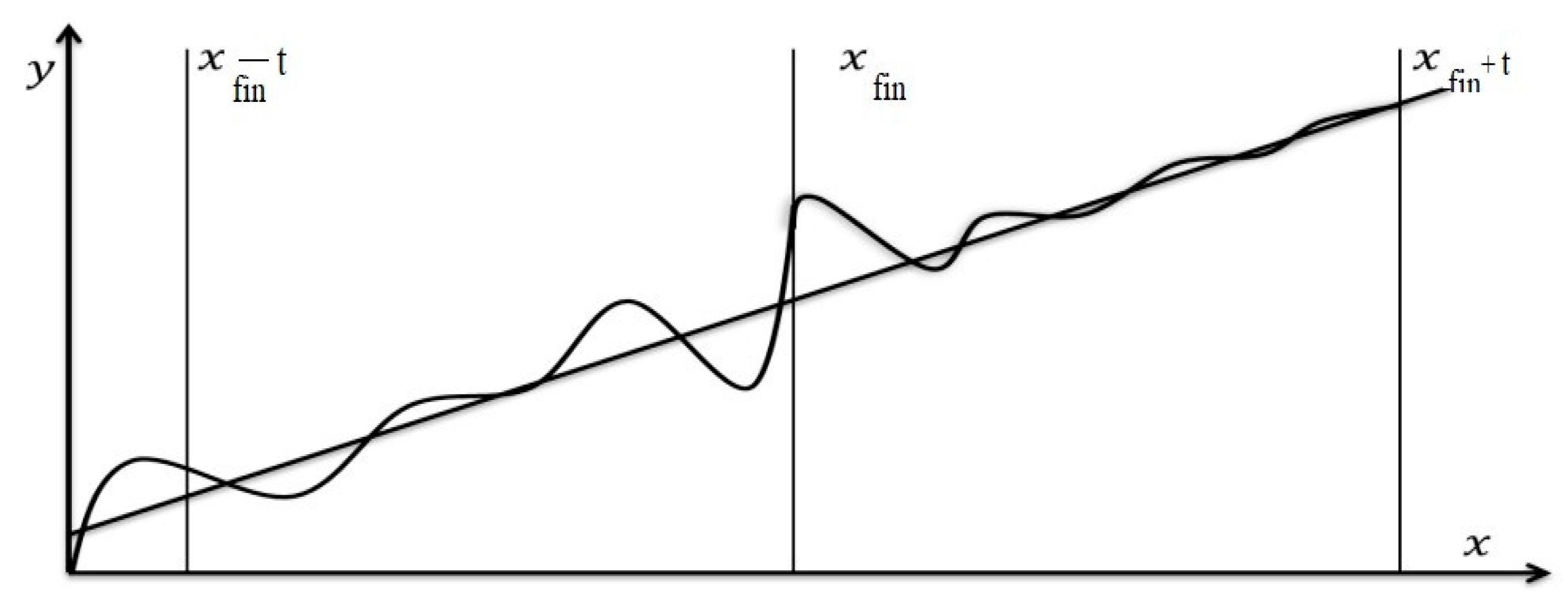
1. Averaged linear forecast (Figure 7). The averaged linear forecast approaches the linear forecast asymptotically, but, unlike the linear forecast, it preserves short-term trends of changes in the function value Equation (21).
where k is the linearity coefficient.
2. Neural forecast. The neural forecast is calculated by selecting the training coefficients based on historical data of the artificial neural network using a combination of optimization (backpropagation of error) and stochastic methods.
The multilayer neural network-based forecast has the form Equation (22):
—prediction function; —calculated coefficients; —rational sigmoid; —the ordinal number of the neural network layer; —the ordinal number of the neural network input; —input width of the neural network; —time interval of the first predicted value ; —main input values of the network; —additional input values.
3. Combined multitrend forecast. A combined multitrend forecast represents the aggregate of linear, logarithmic, and harmonic trends, and is calculated using sequential trend decomposition.
Let us formulate the prediction function as an aggregate of logarithmic, linear, and harmonic trends Equation (23):
where:
Thus, .
The aggregate forecast can be represented as Equation (24):
4.6. The Aggregate Risk Model for an Asset in the Market
The aggregate asset risk is represented as the sum of risks Equation (25):
where: —unconditional risk; —risk of selling an asset at a loss; —risk of the asset value crash.
The unconditional (stochastic) component of risk is classically described as Equation (26):
where: —variance of the asset value for the period .
The risk of selling an asset at a loss is expressed as the product of the probability of selling an asset at a price below by the standard deviation of the value Equation (27).
We estimate the probability as the ratio of the sum of minimum time frames , during which the sale of an asset at a loss is possible, to total in Equation (28).
The risk of the crash that occurs during crisis periods can be estimated based on the dynamics of the crisis, expressed as Equation (29):
whereas in the period of crisis Equation (30):
given that the maximum possible downfall will be at least , or , where: —the maximum drop in the asset value recorded over the historical period ; —Heaviside function: .
Thus, the model’s aggregate risk has the form Equation (31):
The aggregate risk forecast for an asset is calculated in the same way as the aggregate asset value forecast using a relative confidence coefficient.
Then, the problem of forming an adaptive investment strategy portfolio is formulated as follows Equation (32):
where: —the number of assets in the portfolio; —the minimum and maximum allowable number of assets; —portfolio efficiency; —degree of diversification; —the market state; —type of diversification; —aggregate risk of the portfolio; —maximum allowable aggregate risk.
5. Results
To compare the performance of the adaptive investment strategy with the existing classical portfolio strategies, we conducted behavioral modeling of strategic investment portfolios over a 10-year period based on real historical data for 14 years. For comparative analysis, the following types of portfolios were used:
Table 8 provides a comparison of portfolio investment performance.
These results demonstrate the dominance of the dynamic adaptive strategy not only over the static portfolio of H. Markowitz but also over the dynamic, rebalanced portfolio of R. Roll.
From the empirical data, it is evident that the dynamic adaptive strategy has a significant superiority over the strategies of H. Markowitz and R. Roll, even though it needs less rebalancing than R. Roll’s strategy.
The advantage of the adaptive strategy is that it is based on predictive data as opposed to Roll’s strategy, which relies on historical data only. At the same time, it also differs from H. Markowitz’s strategy, where the predictive factor is solely based on the assumption that the asset price will rise in the long term.
For this reason, the main factor of the optimization and rebalancing of the value W is a leading indicator that is considerably superior to the VaR in terms of the indication and timing. In all cases, the change in the W indicator happens much earlier than the VaR extremum is reached, which allows rebalancing the portfolio proactively without waiting for the occurrence of significant losses in the portfolio value.
6. Conclusions
In the time period used, the dynamic adaptive portfolio is guaranteed to have no lower return than the classic H. Markowitz’s portfolio and R. Roll’s portfolio. The evaluation of the movement of the asset value in the portfolio allows us to draw the following conclusions:
1. The greatest efficiency of the dynamic adaptive strategy is revealed during periods of significant market changes (crises and pre-crisis situations).
2. In tranquil market conditions, there is no need to rebalance the dynamic adaptive portfolio since the absence of significant movement in the asset value does not lead to a dramatic change in the W indicator (assessment of the state) of the asset. In this case, the dynamic portfolio will not have superiority over H. Markowitz’s portfolio, but will be inferior in returns to the arbitrage portfolio due to the lack of rebalancing.
3. In times of crisis, the dynamic adaptive portfolio model demonstrates better return performance than the classic portfolio models. However, during periods of a stable market, the models of H. Markowitz and R. Roll are preferable since they do not require additional costs for data collection, processing, and forecasting, and also allow the investor to take a wait-and-see position, that is, to reduce their own time spent on portfolio management to zero.
Thus, the analysis of the results showed a comparative advantage of the dynamic adaptive strategy over models based on classical concepts.
The adaptive investment strategy allows one to respond to the changing conditions of the investment environment in time. However, it should be noted that such a strategy requires the constant attention of the investor and timely response to the signal initiation, which entails spending extra time and resources of the investor. The adaptive investment strategy allows one to reduce the risk of losing one’s invested funds. This can be explained by the fact that an acceptable level of losses is set by the investors themselves, and when a given level of losses is reached, the portfolio is rebalanced, which allows the investor to save their invested capital.
Supplementary Materials
The following are available online at https://www.mdpi.com/article/10.3390/economies9030095/s1, Figure S1: Crisis phase identification.
Funding
This research received no external funding.
Informed Consent Statement
Not applicable.
Data Availability Statement
Not applicable.
Conflicts of Interest
The author confirms that there is no conflict of interests to declare for this publication.
References
- Abdollahi, Hooman. 2020. A novel hybrid model for forecasting crude oil price based on time series decomposition. Applied Energy 267: 115035. [Google Scholar] [CrossRef]
- Benita, Francisco, Francisco López-Ramos, and Stefano Nasini. 2019. A bi-level programming approach for global investment strategies with financial intermediation. European Journal of Operational Research 274: 375–90. [Google Scholar] [CrossRef]
- Bi, Junna, and Cai Jun. 2019. Optimal investment–reinsurance strategies with state dependent risk aversion and VaR constraints in correlated markets. Insurance: Mathematics and Economics 85: 1–14. [Google Scholar] [CrossRef]
- Borovička, Adam. 2020. New complex fuzzy multiple objective programming procedure for a portfolio making under uncertainty. Applied Soft Computing 96: 106607. [Google Scholar] [CrossRef]
- Cesarone, Francesco, Fabiomassimo Mango, Carlo Domenico Mottura, Jacopo Maria Ricci, and Fabio Tardella. 2020. On the stability of portfolio selection models. Journal of Imperial Finance 59: 210–34. [Google Scholar]
- Chang, Jinhua, Lin Sun, Bo Zhang, and Jin Pengb. 2020. Multi-period portfolio selection with mental accounts and realistic constraints based on uncertainty theory. Journal of Computational and Applied Mathematics 377: 112892. [Google Scholar] [CrossRef]
- Chen, Shun, and Lei Ge. 2021. A learning-based strategy for portfolio selection. International Review of Economics & Finance 71: 936–42. [Google Scholar]
- Chu, Gang, Wei Zhang, Guofeng Sun, and Xiaotao Zhang. 2019. A new online portfolio selection algorithm based on Kalman Filter and anti-correlation. Physica A: Statistical Mechanics and its Applications 536: 120949. [Google Scholar] [CrossRef]
- Dai Pra, Paolo, and Marco Tolotti. 2009. Heterogeneous credit portfolios and the dynamics of the aggregate losses. Stochastic Processes and their Applications 119: 2913–44. [Google Scholar] [CrossRef] [Green Version]
- De Leeuw, Tim, Victor Gilsing, and Geert Duysters. 2019. Greater adaptivity or greater control? Adaptation of IOR portfolios in response to technological change. Research Policy 48: 1586–600. [Google Scholar]
- Eom, Cheoljun, and Jong Won Park. 2019. A new method for better portfolio investment: A case of the Korean stock market. Pacific-Basin Finance Journal 49: 213–31. [Google Scholar] [CrossRef]
- Gataullin, Timur M., Sergey T. Gataullin, and Ksenia V. Ivanova. 2020. Modeling an Electronic Auction. In Institute of Scientific Communications Conference. Cham: Springer, pp. 1108–17. [Google Scholar]
- Golosnoy, Vasyl, Bastian Gribisch, and Miriam Isabel Seiferta. 2019. Exponential smoothing of realized portfolio weights. Journal of Empirical Finance 53: 222–37. [Google Scholar] [CrossRef]
- Gong, Xiaomin, Changrui Yu, Liangyu Min, and Zhipeng Ge. 2021. Regret theory-based fuzzy multi-objective portfolio selection model involving DEA cross-efficiency and higher moments. Applied Soft Computing 100: 106958. [Google Scholar] [CrossRef]
- Gorodetskaya, Olga Y., Gulnara I. Alekseeva, Kira A. Artamonova, Natalia A. Sadovnikova, Svetlana G. Babich, Elvira N. Iamalova, and Anatoliy M. Tarasov. 2021. Investment Attractiveness of the Russian Energy Sector MNCs: Assessment and Challenges. International Journal of Energy Economics and Policy 11: 199. [Google Scholar] [CrossRef]
- Guan, Hao, and An Zhiyong. 2019. A local adaptive learning system for online portfolio selec-tion. Knowledge-Based Systems 186: 104958. [Google Scholar] [CrossRef]
- Hadhri, Sinda, and Zied Ftiti. 2019. Asset allocation and investment opportunities in emerging stock mar-kets: Evidence from return asymmetry-based analysis. Journal of International Money and Finance 93: 187–200. [Google Scholar] [CrossRef]
- Ivanyuk, Vera, and Anatoly Tsvirkun. 2013. Intelligent system for financial time series prediction and identification of periods of speculative growth on the financial market. IFAC Proceedings 46: 1128–33. [Google Scholar] [CrossRef]
- Jeon, Junkee, and Yong Hyun Shin. 2019. Finite horizon portfolio selection with a negative wealth constraint. Journal of Computational and Applied Mathematics 356: 329–38. [Google Scholar] [CrossRef]
- Khedmati, Majid, and Pejman Azin. 2020. An online portfolio selection algorithm using clustering approaches and considering transaction costs. Expert Systems with Applications 159: 113546. [Google Scholar] [CrossRef]
- Li, Bo, Yufei Sun, Grace Aw, and Kok Lay Teo. 2019. Uncertain portfolio optimization problem under a minimax risk measure. Applied Mathematical Modelling 76: 274–81. [Google Scholar] [CrossRef]
- Lu, Ya-Nan, Sai-Ping Li, Li-Xin Zhong, Xiong-Fei Jiang, and Fei Ren. 2018. A clustering-based portfolio strategy incorporating momentum effect and market trend prediction. Chaos, Solitons & Fractals 117: 1–15. [Google Scholar]
- Lu, Richard, Vu Tran Hoang, and Wing-Keung Wong. 2020. Do lump-sum investing strategies really outperform dollar-cost averaging strategies? Studies in Economics and Finance. [Google Scholar] [CrossRef]
- Ma, Guiyuan, Chi Chung Siu, and Song-Ping Zhu. 2019. Dynamic portfolio choice with return predictability and trans-action costs. European Journal of Operational Research 278: 976–88. [Google Scholar] [CrossRef]
- Ma, Yilin, Ruizhu Han, and Weizhong Wang. 2021. Portfolio optimization with return prediction using deep learning and machine learning. Expert Systems with Applications 165: 113973. [Google Scholar] [CrossRef]
- Mansour, Nabil, Mohamed Sadok Cherif, and Walid Abdelfattah. 2019. Multi-objective impre-cise programming for financial portfolio selection with fuzzy returns. Expert Systems with Applications 138: 112810. [Google Scholar] [CrossRef]
- Markowitz, Harry. 1952. Portfolio Selection. Journal of Finance 7: 77–91. [Google Scholar] [CrossRef]
- Mishra, Sasmita, and Sudarsan Padhy. 2019. An efficient portfolio construction model using stock price predicted by support vector regression. The North American Journal of Economics and Finance 50. [Google Scholar] [CrossRef]
- Mo, Guoli, Chunzhi Tan, Weiguo Zhang, and Fang Liu. 2019. International portfolio of stock indices with spatiotemporal correlations: Can investors still benefit from portfolio, when and where? The North American Journal of Economics and Finance 47: 168–83. [Google Scholar] [CrossRef]
- Paiva, Felipe Dias, Rodrigo Tomás Nogueira Cardoso, Gustavo Peixoto Hanaoka, and Wendel Moreira Duarte. 2019. Decision-making for financial trading: A fusion approach of machine learning and portfolio selection. Expert Systems with Applications 115: 635–55. [Google Scholar] [CrossRef]
- Park, Hyungjun, Min Kyu Sim, and Dong Gu Choi. 2020. An intelligent financial portfolio trading strategy using deep Q-learning. Expert Systems with Applications 158: 113573. [Google Scholar] [CrossRef]
- Puerto, Justo, Moisés Rodríguez-Madrena, and Andrea Scozzari. 2020. Clustering and portfolio selection problems: A unified framework. Computers & Operations Research 117: 104891. [Google Scholar]
- Roll, Richard. 1977. A critique of the asset pricing theory’s tests Part I: On past and potential testability of the theory. Journal of Financial Economics 4: 129–76. [Google Scholar] [CrossRef]
- Sunchalin, Andrew M., Rasul A. Kochkarov, Kirill G. Levchenko, Azert. A. Kochkarov, and Vera A. Ivanyuk. 2019. Methods of risk management in portfolio theory. Revista Espacios 40: 25. [Google Scholar]
- Wang, Minggang, Longfeng Zhao, Ruijin Du, Chao Wang, Lin Chen, Lixin Tian, and H. Eugene Stanley. 2018. A novel hybrid method of forecasting crude oil prices using complex network science and artificial intelligence algorithms. Applied Energy 220: 480–95. [Google Scholar] [CrossRef]
- Wei, Jiuchang, Bing Bu, and Liang Liang. 2012. Estimating the diffusion models of crisis information in micro blog. Journal of Informetrics 6: 600–10. [Google Scholar] [CrossRef]
- Wu, Yu Xi, Qing Biao Wu, and Jia-Qi Zhu. 2019. Improved EEMD-based crude oil price forecasting using LSTM networks. Physica A: Statistical Mechanics and Its Applications 516: 114–24. [Google Scholar] [CrossRef]
- Yerznkyan, Bagrat, Svetlana Bychkova, Timur Gataullin, and Sergey Gataullin. 2019. The sufficiency principle as the ideas quintessence of the club of Rome. Montenegrin Journal of Economics 15: 21–29. [Google Scholar] [CrossRef]
- Yerznkyan, Begrat, Timur M. Gataullin, and Sergey T. Gataullin. 2021. Solow Models with Linear Labor Function for Industry and Enterprise. Montenegrin Journal of Economics 17: 111–20. [Google Scholar] [CrossRef]
- Yu, Xingying, Yang Shen, Xiang Li, and Kun Fan. 2020. Portfolio selection with parameter uncertainty under α maxmin mean–variance criterion. Operations Research Letters 48: 720–24. [Google Scholar] [CrossRef]
- Zhou, Wei, and Zeshui Xu. 2018. Portfolio selection and risk investment under the hesitant fuzzy environment. Knowledge-Based Systems 144: 21–31. [Google Scholar] [CrossRef]
- Zhu, Jiaming, Jinpei Liu, Peng Wu, Huayou Chen, and Ligang Zhou. 2019. A novel decomposition-ensemble approach to crude oil price forecasting with evolution clustering and combined model. International Journal of Machine Learning and Cybernetics 10: 3349–62. [Google Scholar] [CrossRef]
- Zhu, Shushang, Wei Zhu, Xi Pei, and Xueting Cui. 2020. Hedging crash risk in optimal portfolio selection. Journal of Banking & Finance 119: 105905. [Google Scholar]
Figure 1.
The concept of an innovative investment strategy adaptable to changes in the market situation.
Figure 1.
The concept of an innovative investment strategy adaptable to changes in the market situation.

Figure 2.
Portfolio construction algorithm for an adaptive strategy investment portfolio.

Figure 3.
Possible results of the market analysis function.

Figure 4.
Dynamic stagnation model.

Figure 5.
Growth and decline model.

Figure 6.
Crisis Model.

Figure 7.
Averaged linear forecast.

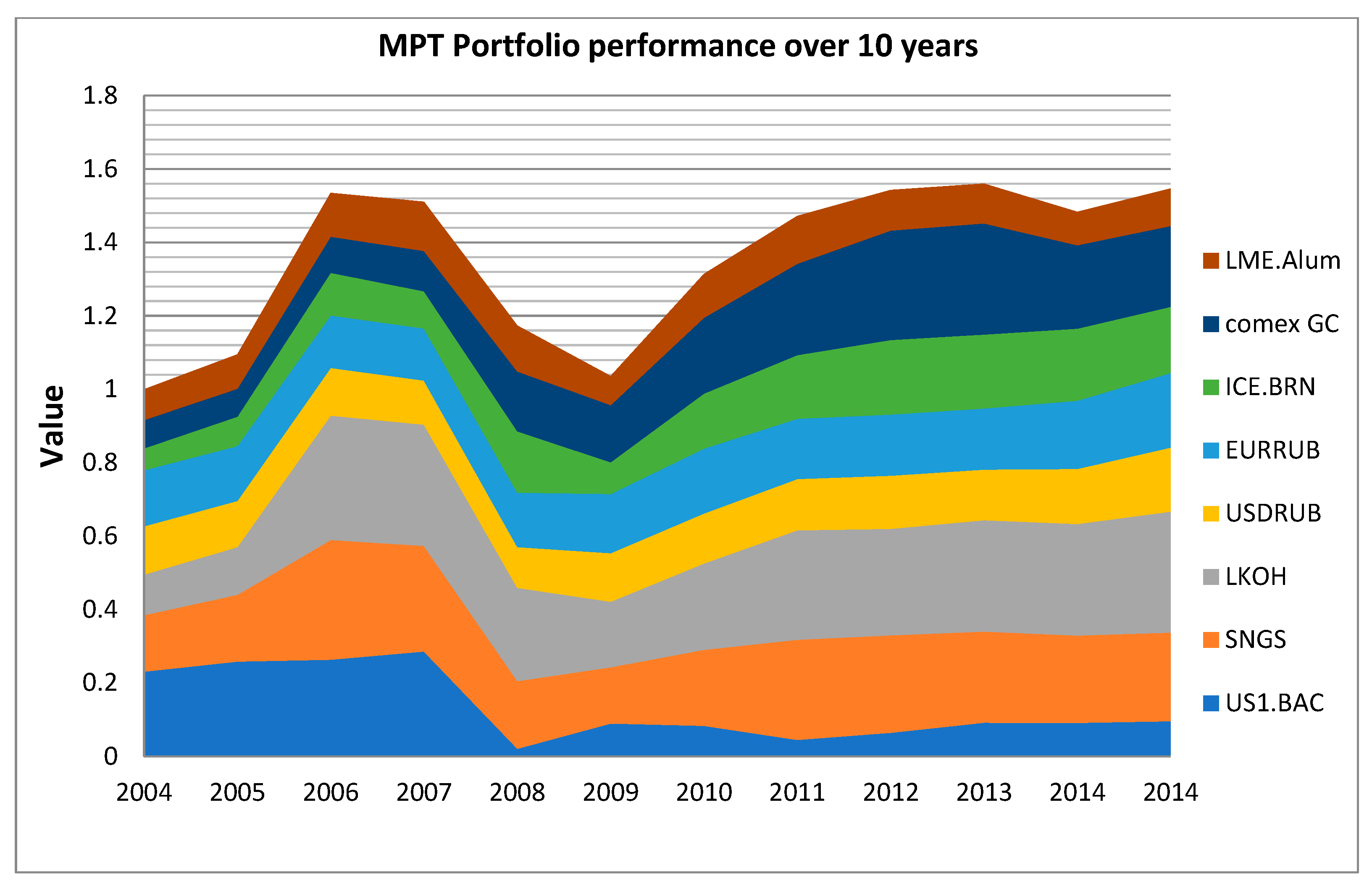
Figure 8.
MPT Portfolio. Total portfolio return: 54.7%. Highest return achieved: 56%. Number of rebalancing events: 0. LME Alum—physical aluminum (contracts); Comex GC—physical gold (contracts); ICE BRN—Brent crude oil (contracts); EUR RUB—Euro (currency); USD RUB—US dollar (currency); LKOH—shares of Lukoil (shares); SNGS—shares of Surgutneftegaz (shares); US1 BAC—Bank of America shares (shares).

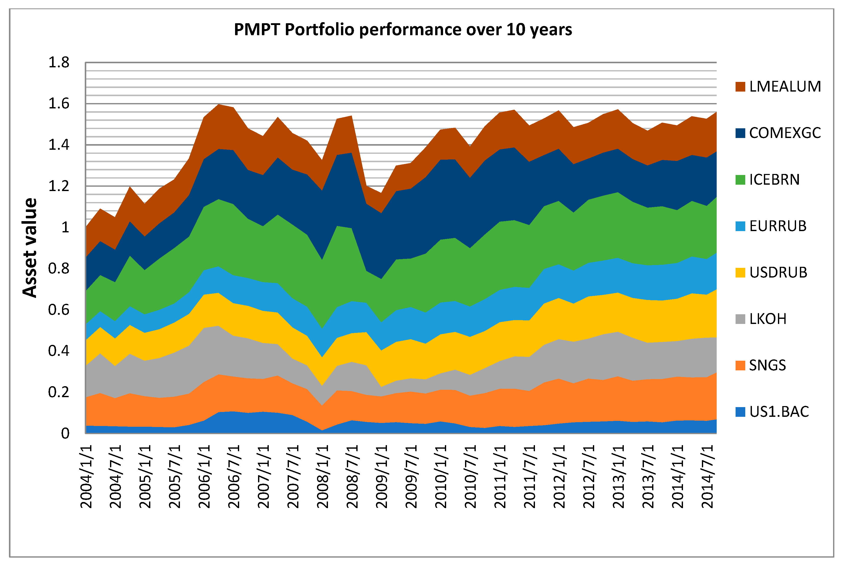
Figure 9.
PMPT Portfolio. Total portfolio return: 55.9%. Highest return achieved: 59.7%. Number of rebalancing events: 40. LME Alum—physical aluminum (contracts); Comex GC—physical gold (contracts); ICE BRN—Brent crude oil (contracts); EUR RUB—Euro (currency); USD RUB—US dollar (currency); LKOH—shares of Lukoil (shares); SNGS—shares of Surgutneftegaz (shares); US1 BAC—Bank of America shares (shares).

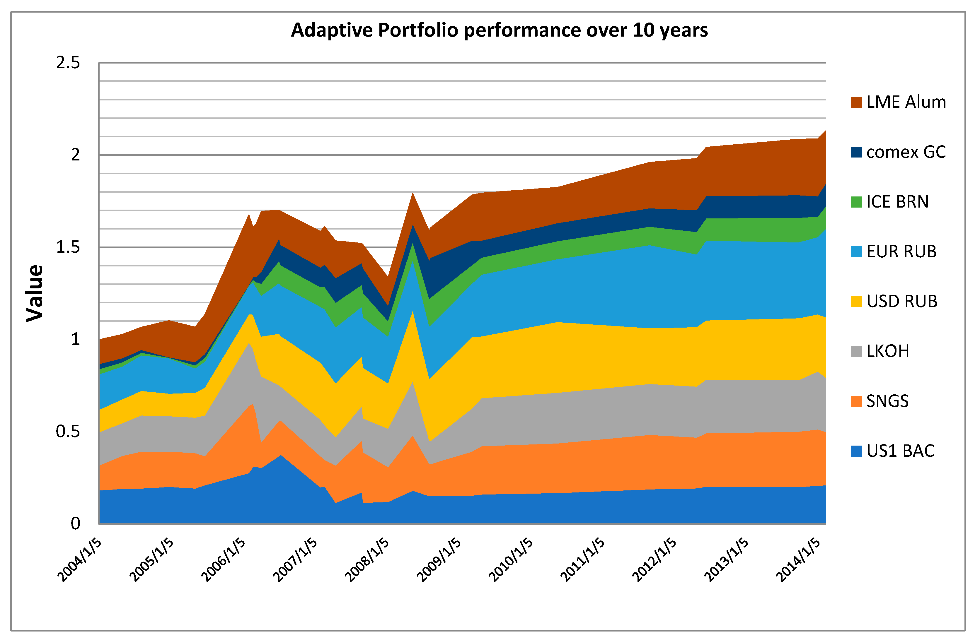
Figure 10.
Adaptive Portfolio. Total portfolio return: 113.4%. Highest return achieved: 113.4%. Number of rebalancing events: 30. LME Alum—physical aluminum (contracts); Comex GC—physical gold (contracts); ICE BRN—Brent crude oil (contracts); EUR RUB—Euro (currency); USD RUB—US dollar (currency); LKOH—shares of Lukoil (shares); SNGS—shares of Surgutneftegaz (shares); US1 BAC—Bank of America shares (shares).


Table 1.
Boundaries of basic states.
| Market State | |
|---|---|
| Speculative growth | |
| Growth | |
| Dynamic stagnation | 0.5 |
| Decline | |
| Crisis decline |
Table 2.
Investment portfolio strategy selection with regard to the market state.
| Market State | Profit-Taking | Portfolio Risk | Type of Diversification | Degree of Diversification | Portfolio Dynamicity |
|---|---|---|---|---|---|
| Speculative growth | Growing portfolio | Very high | Naive | Very low | Very low |
| Growth | Weakly bounded portfolio | High | Grouped | Low | Low |
| Stagnation | Bounded portfolio | Moderate | Jurisdictional | Moderate | Moderate |
| Decline | Highly bounded portfolio | Low | Covariant | High | High |
| Crisis decline | Fixed portfolio | Very low | Beta Neutral | Very high | Very high |
Table 3.
Types of diversification by the degree of risk increase.
| Risk | Type of Diversification | |
|---|---|---|
| 0 | Minimum | Beta-neutral |
| 1 | Low | Covariant |
| 2 | Moderate | Jurisdictional |
| 3 | High | Industry-based |
| 4,5 | Maximum | Naive |
Table 4.
Compliance of portfolio strategy with the current market situation.
| Market State | Weight of the Market State | Profit-Taking | Portfolio Risk | Type of Diversification | Degree of Diversification | Portfolio Dynamicity |
|---|---|---|---|---|---|---|
| Speculative growth | 1 | 0.2 | 0.2 | 0.2 | 0.2 | 0.2 |
| Growth | 0.75 | 0.15 | 0.15 | 0.15 | 0.15 | 0.15 |
| Stagnation | 0.5 | 0.1 | 0.1 | 0.1 | 0.1 | 0.1 |
| Decline | 0.25 | 0.05 | 0.05 | 0.05 | 0.05 | 0.05 |
| Crisis decline | 0 | 0 | 0 | 0 | 0 | 0 |
Table 5.
Input data for H. Markowitz’s portfolio.
| Portfolio | Markowitz’s Portfolio |
|---|---|
| Strategy | Buy and Hold |
| Rebalancing | By bankruptcy |
| Diversification limit | 90.0% |
| Risk limit | 15% |
| Minimum asset share | 0.1% |
| Transaction costs | 0.2% |
| Optimization | By rate of return |
| Investment term | 10 years |
| Start of Investment | 2004 |
Table 6.
Input data for PMPT portfolio.
| Portfolio | PMPT |
|---|---|
| Strategy | Periodic Rebalancing |
| Rebalancing | On quarterly basis |
| Diversification limit | 90.0% |
| Risk limit | 20% |
| Minimum asset share | 0.1% |
| Transaction costs | 0.2% |
| Optimization | By the VaR criterion |
| Investment term | 10 years |
| Start of Investment | 2004 |
Table 7.
Input data for adaptive dynamic portfolio model.
| Portfolio | Dynamic |
|---|---|
| Strategy | Dynamic |
| Rebalancing | By changes in W (market state) |
| Diversification limit | 90.0% |
| Risk limit | 20% |
| Minimum asset share | 0.1% |
| Transaction costs | 0.2% |
| Optimization | By W criterion (market state) |
| Investment term | 10 years |
| Start of Investment | 2004 |
Table 8.
Comparison of portfolio investment performance.
| Portfolio Type | Average Annual Return | Number of Rebalancing Events |
|---|---|---|
| H. Markowitz’s portfolio | 5.47% | 0 |
| R. Roll’s portfolio | 5.59% | 45 |
| Dynamic portfolio | 11.3% | 30 |
Publisher’s Note: MDPI stays neutral with regard to jurisdictional claims in published maps and institutional affiliations. |
© 2021 by the author. Licensee MDPI, Basel, Switzerland. This article is an open access article distributed under the terms and conditions of the Creative Commons Attribution (CC BY) license (https://creativecommons.org/licenses/by/4.0/).
Share and Cite
MDPI and ACS Style
Ivanyuk, V. Formulating the Concept of an Investment Strategy Adaptable to Changes in the Market Situation. Economies 2021, 9, 95. https://0-doi-org.brum.beds.ac.uk/10.3390/economies9030095
AMA Style
Ivanyuk V. Formulating the Concept of an Investment Strategy Adaptable to Changes in the Market Situation. Economies. 2021; 9(3):95. https://0-doi-org.brum.beds.ac.uk/10.3390/economies9030095
Chicago/Turabian StyleIvanyuk, Vera. 2021. "Formulating the Concept of an Investment Strategy Adaptable to Changes in the Market Situation" Economies 9, no. 3: 95. https://0-doi-org.brum.beds.ac.uk/10.3390/economies9030095
Note that from the first issue of 2016, this journal uses article numbers instead of page numbers. See further details here.