A Two-Sample Test of High Dimensional Means Based on Posterior Bayes Factor

Abstract

In classical statistics, the primary test statistic is the likelihood ratio. However, for high dimensional data, the likelihood ratio test is no longer effective and sometimes does not work altogether. By replacing the maximum likelihood with the integral of the likelihood, the Bayes factor is obtained. The posterior Bayes factor is the ratio of the integrals of the likelihood function with respect to the posterior. In this paper, we investigate the performance of the posterior Bayes factor in high dimensional hypothesis testing through the problem of testing the equality of two multivariate normal mean vectors. The asymptotic normality of the linear function of the logarithm of the posterior Bayes factor is established. Then we construct a test with an asymptotically nominal significance level. The asymptotic power of the test is also derived. Simulation results and an application example are presented, which show good performance of the test. Hence, taking the posterior Bayes factor as a statistic in high dimensional hypothesis testing is a reasonable methodology.

1. Introduction

The likelihood ratio is the primary test statistic in hypothesis testing owing to its dominating power. However, for high dimensional data, the likelihood ratio statistic is sometimes undefined. For example, the likelihood function of a multivariate normal distribution is unbounded when the dimension of data is greater than the sample size. Even if the likelihood ratio is well-defined, its performance is unsatisfactory when the dimension is proportionally “close to" the sample size [1]. Therefore, when the dimension is large relative to the sample size, that is the so-called “large p small n” situation; how to choose a test statistic plays a key role in statistical inference.

In this article, we try to use the posterior Bayes factor to be a test statistic for high dimensional data, applying it to equality testing of two multivariate normal mean vectors. The classical likelihood ratio test statistic is the ratio of the maximum values of likelihoods, whereas the Bayes factor is the ratio of the integrated likelihoods. We chose the posterior Bayes factor rather than the prior Bayes factor because when the dimension is fixed, the former is less affected by the variations of the prior. This paper aims to investigate the ability of the posterior Bayes factor as a test statistic. As a result, a simple prior is taken for the parameter.

In multivariate analysis, testing the equality of two means is a fundamental problem. The classical procedure for this problem is the famous Hotelling T${}^2$ test in [2], which is based on Mahalanobis distance between the sample mean vectors weighted by the inverse sample covariance matrix. Hotelling’s T${}^2$ test is the most powerful invariant test when the dimension is fixed and much smaller than the total sample size [3], but it is unsatisfactory when the dimension is large relative to the sample size [1]. However, in recent decades, hypothesis testing viable for high dimensional data is increasingly demanded in many application areas such as genomics, finance, medicine, and so on. An important work [1] modifies Hotelling’s T${}^2$ statistic in a high dimensional setting by removing the inverse of the sample covariance from the Hotelling formulation. Some new test statistics for the mean vector are introduced by replacing the sample covariance with its diagonal in [4,5,6]. In [7], a statistic is constructed by retaining the cross-product terms in work [1]. In the sequel, ref. [8] standardizes each component of $\overline{X}-\overline{Y}$ in [7] by the corresponding variance estimation and proposes a scale-invariant test. The test statistics introduced above are called “sum-of-squares type statistics” (see [9]) and attempt to get around the ill-formed sample covariance matrix. Another major approach called “projecting data” transforms high dimensional data into low dimensional data with random projection so that traditional tests can be applied. See, for example [10,11,12]. By maximizing an average signal to noise ratio, ref. [13] finds the optimal projection subspace and proposes a new test procedure based on it. Besides the two main approaches mentioned above, ref. [14] studies the rates of convergence for the high-dimensional mean and proposes tests based on the sample mean. A new test based on random subspaces is proposed by [15]. A generalized component test is presented in [16], whose statistic is the average of the squared t-statistics for all the component testing problems. A method using a multiple hypothesis test based on the maximum of standardized partial sums of logarithmic p-values statistic is introduced in [17]. More works about testing the mean vectors are presented in [18,19,20].

Few articles develop tests for the means of two samples with Bayesian machineries in high dimensional settings. A Bayes factor-based testing procedure is developed by [12]. However, the statistic is still constructed with lower dimensional random projections of the high dimensional data vectors because Bayes factors based on Jeffrey’s prior involve inversion of the ill-formed sample covariance matrices, as in the classical Hotelling T${}^2$ test statistic in a “large p small n” setting. The approach of random projection cannot be applied when the difference of two mean vectors is dense. However, whether the difference of two mean vectors is dense or sparse is not known in applications. Aitkin [21] proposed the posterior Bayes factor, which is the ratio of the posterior means of the likelihood under each model rather than the usual prior means. Suppose two models $M_0$ and $M_1$ for common data x are considered, under which the likelihood function is $L_i\left({\mathit{\theta }}_j\right)$, where ${\mathit{\theta }}_j$ is the parameter of dimension $p_j$ and belongs to the parameter space ${\Theta }_j,j\in \{0,1\}$. Specifying prior ${\pi }_j\left({\mathit{\theta }}_j\right)$ to ${\mathit{\theta }}_j$, $j\in \{0,1\}$, then the posterior Bayes factor in favor of the model $M_1$, denoted by PBF${}_{10}$, is defined as

$${\mathrm{PBF}}_{10}=\frac{{\overline{L}}_1}{{\overline{L}}_0},$$

(1)

where ${\overline{L}}_j$ is the posterior mean:

$${\overline{L}}_j={\int }_{{\Theta }_j}{L}_j\left({\mathit{\theta }}_j\right){\pi }_j\left({\mathit{\theta }}_j\right|x,y)\mathrm{d}{\mathit{\theta }}_j,j\in \{0,1\},$$

and ${\pi }_j\left({\mathit{\theta }}_j\right|x,y)$ is the posterior density of ${\mathit{\theta }}_j$:

$${\pi }_j\left({\mathit{\theta }}_j\right|x,y)=\frac{L_j\left({\mathit{\theta }}_j\right){\pi }_j\left({\mathit{\theta }}_j\right)\mathrm{d}{\mathit{\theta }}_j}{{\int }_{{\Theta }_j}{L}_j\left({\mathit{\theta }}_j\right){\pi }_j\left({\mathit{\theta }}_j\right)\mathrm{d}{\mathit{\theta }}_j},j\in \{0,1\}.$$

(2)

Unlike the Bayes factor, which is highly dependent on the prior and may be very sensitive to variations in the prior, the posterior Bayes factor reduces this sensitivity to the prior. Specifically, when model $M_0$ is a regular submodel of $M_1$, the logarithm of the posterior Bayes factor under model $M_1$ has

$$2ln{\mathrm{PBF}}_{10}\stackrel{d}{\to }-vln2+{\chi }^2\left(v\right),$$

where “$\stackrel{d}{\to }$” means the convergence in distribution, and $v=p_1-p_0$ and ${\chi }^2\left(v\right)$ denotes a Chi-square distribution with v degrees of freedom. The asymptotic distribution of the logarithm of the posterior Bayes factor is independent of the prior distribution, which further illustrates that the posterior Bayes factor is insensitive to the prior.

Inspired by [21], we consider testing the equality of two high dimensional means with the posterior Bayes factor. With an appropriate prior, the posterior Bayes factor no longer suffers the impediment of the inversion of ill-formed matrices. Additionally, compared with the approach in [12], which proposed a test based on the Bayes factor with random projections, the posterior Bayes factor can be applied for both dense and sparse cases. In this paper, a non-informative prior also works for the location parameters, while an inverse Wishart prior is taken for the covariance matrix. We establish the asymptotic normality of the logarithm of the posterior Bayes factor under the null hypothesis and derive the asymptotic power of the test. Simulation studies are carried out to investigate the performance of the proposed test. The numerical results show that the power of our test outperforms the competitors in most cases.

The rest of this article is organized as follows. In Section 2, we derive the posterior Bayes factor for testing the equality of two mean vectors in the “large p small n” setting. The asymptotic null distribution of the posterior Bayes factor and the local power function of the test are also presented. Simulation results are given in Section 3. We apply the proposed test to a real dataset in Section 4. Section 5 concludes the paper. Technical proofs and the code for performing the simulation studies are deferred to Appendix A and Appendix B.

2. Test Based on Posterior Bayes Factor

This section tries to construct the test based on the posterior Bayes factor. Let $X=(X_1,\dots ,X_{n_1})$ and $Y=(Y_1,\dots ,Y_{n_2})$ be iid samples from p-dimensional multivariate normal distributions $N_p({\mu }_1,\Sigma )$ and $N_p({\mu }_2,\Sigma )$, respectively, where ${\mu }_1$ and ${\mu }_2$ are $p\times 1$ vectors, and $\Sigma$ is a positively definite $p\times p$ matrix. The goal is to test the hypotheses

$$H_0:{\mu }_1={\mu }_2\mathrm{versus}{H}_1:{\mu }_1\ne {\mu }_2.$$

(3)

In order to test Hypotheses (3) by the posterior Bayes factor, we specify the priors for the parameters ${\mu }_1$, ${\mu }_2$ and $\Sigma$ under both the null and alternative hypotheses as

$${\pi }_0\left(\mu \right)=1,\Sigma \sim W_p^{-1}(m_0,V^{-1}),$$

(4)

and

$${\pi }_1\left({\mu }_1\right)={\pi }_1\left({\mu }_2\right)=1,\Sigma \sim W_p^{-1}(m_1,V^{-1}),$$

(5)

respectively, where $\mu$ is the common mean vector under the null hypothesis, and $W_p^{-1}(m_j,V^{-1})$ is the inverse Wishart distribution with real degrees of freedom $m_j$ and a positive definite matrix $V^{-1}$, $j\in \{0,1\}$.

The reasons for choosing the above priors are as follows.

• When no knowledge about the prior is available, a non-informative prior is suggested. A usual one is Jeffrey’s prior. As a result, for the parameters ${\mu }_1$, ${\mu }_2$, and the common parameter $\mu$ under the null hypothesis, we choose Jeffrey’s prior, i.e., Lebesgue measure.
• For the covariance matrix $\Sigma$, the posterior distribution with Jeffrey’s prior does not exist when $p>n-2$, where $n=n_1+n_2$. Therefore, we take the inverse Wishart distribution, which is a conjugate for a normal covariance matrix.
• This paper aims to investigate whether the test with the posterior Bayes factor statistic in high dimensional settings performs better than the existing methods. If the results turn out to be as expected, the posterior Bayes factor could be suggested to be the test statistic for high dimensional datasets. Hence, we will take simple priors. Furthermore, we take $V=k{\mathrm{I}}_p$ in the priors for the covariance matrices with small k so that the variation of the $\Sigma$ is large.

The joint densities of X and Y under the null and alternative hypotheses are

$${\left(2\pi \right)}^{-\frac{np}{2}}{|\Sigma |}^{-\frac{n}{2}}exp\left\{-\frac{1}{2}\mathrm{tr}{\Sigma }^{-1}\left[\sum _{i=1}^{n_1}(x_i-\mu ){(x_i-\mu )}^T+\sum _{i=j}^{n_2}(y_j-\mu ){(y_j-\mu )}^T\right]\right\}$$

and

$${\left(2\pi \right)}^{-\frac{np}{2}}{|\Sigma |}^{-\frac{n}{2}}exp\left\{-\frac{1}{2}\mathrm{tr}{\Sigma }^{-1}\left[\sum _{i=1}^{n_1}(x_i-{\mu }_1){(x_i-{\mu }_1)}^T+\sum _{i=j}^{n_2}(y_j-{\mu }_2){(y_j-{\mu }_2)}^T\right]\right\},$$

respectively. Then the posterior mean ${\overline{L}}_1$ under $H_1$ can be calculated as

$${\overline{L}}_1={\int }_{{\Theta }_1}{L}_1\left({\mathit{\theta }}_1\right)\left[\frac{L_1\left({\mathit{\theta }}_1\right){\pi }_1\left({\mathit{\theta }}_1\right)}{{\int }_{{\Theta }_1}{L}_1\left({\mathit{\theta }}_1\right){\pi }_1\left({\mathit{\theta }}_1\right)\mathrm{d}{\mathit{\theta }}_1}\right]\mathrm{d}{\mathit{\theta }}_1=\frac{{\int }_{{\Theta }_1}{L}_1^2\left({\mathit{\theta }}_1\right){\pi }_1\left({\mathit{\theta }}_1\right)\mathrm{d}{\mathit{\theta }}_1}{{\int }_{{\Theta }_1}{L}_1\left({\mathit{\theta }}_1\right){\pi }_1\left({\mathit{\theta }}_1\right)\mathrm{d}{\mathit{\theta }}_1},$$

where

$$\begin{array}{cc}\hfill & {\int }_{{\Theta }_1}{L}_1\left({\mathit{\theta }}_1\right){\pi }_1\left({\mathit{\theta }}_1\right)\mathrm{d}{\mathit{\theta }}_1\hfill \\ \hfill =& {\left(2\pi \right)}^{-\frac{(n-2)p}{2}}{n}_1^{-\frac{p}{2}}{n}_2^{-\frac{p}{2}}\frac{2^{\frac{(m_1+n-2)p}{2}}{|V^{-1}+S_1+S_2|}^{-\frac{m_1+n-2}{2}}{\Gamma }_p\left(\frac{m_1+n-2}{2}\right)}{2^{\frac{m_{1}p}{2}}{\left|V\right|}^{\frac{m_1}{2}}{\Gamma }_p\left(\frac{m_1}{2}\right)},\hfill \end{array}$$

and ${\Gamma }_p(·)$ denotes the multivariate gamma function, that is,

$${\Gamma }_p\left(a\right)={\pi }^{p(p-1)/4}\prod _{j=1}^p\Gamma [a+(1-j)/2].$$

$$S_1=\sum _{i=1}^{n_1}(X_i-\overline{X}){(X_i-\overline{X})}^T,S_2=\sum _{j=1}^{n_2}(Y_j-\overline{Y}){(Y_j-\overline{Y})}^T$$

with $\overline{X}={\sum }_{i=1}^{n_1}{X}_i/n_1$, $\overline{Y}={\sum }_{j=1}^{n_2}{Y}_j/n_2$, and

$$\begin{array}{cc}\hfill & {\int }_{{\Theta }_1}{L}_1^2\left({\mathit{\theta }}_1\right){\pi }_1\left({\mathit{\theta }}_1\right)\mathrm{d}{\mathit{\theta }}_1\hfill \\ \hfill =& {\left(2\pi \right)}^{-\frac{(2n-2)p}{2}}{\left(2n_1\right)}^{-\frac{p}{2}}{\left(2n_2\right)}^{-\frac{p}{2}}\frac{2^{\frac{(m_1+2n-2)p}{2}}{|V^{-1}+2S_1+2S_2|}^{-\frac{m_1+2n-2}{2}}{\Gamma }_p\left(\frac{m_1+2n-2}{2}\right)}{2^{\frac{m_{1}p}{2}}{\left|V\right|}^{\frac{m_1}{2}}{\Gamma }_p\left(\frac{m_1}{2}\right)}.\hfill \end{array}$$

The posterior mean ${\overline{L}}_0$ under $H_0$ can be calculated as

$${\overline{L}}_0=\frac{{\int }_{{\Theta }_0}{L}_0^2\left({\mathit{\theta }}_0\right){\pi }_0\left({\mathit{\theta }}_0\right)\mathrm{d}{\mathit{\theta }}_0}{{\int }_{{\Theta }_0}{L}_0\left({\mathit{\theta }}_0\right){\pi }_0\left({\mathit{\theta }}_0\right)\mathrm{d}{\mathit{\theta }}_0},$$

where

$$\begin{array}{cc}\hfill & {\int }_{{\Theta }_0}{L}_0\left({\mathit{\theta }}_0\right){\pi }_0\left({\mathit{\theta }}_0\right)\mathrm{d}{\mathit{\theta }}_0\hfill \\ \hfill =& {\left(2\pi \right)}^{-\frac{(n-1)p}{2}}{n}^{-\frac{p}{2}}\frac{2^{\frac{(m_0+n-1)p}{2}}{|V^{-1}+S_1+S_2+\frac{n_1{n}_2}{n}(\overline{X}-\overline{Y}){(\overline{X}-\overline{Y})}^T|}^{-\frac{m_0+n-1}{2}}{\Gamma }_p\left(\frac{m_0+n-1}{2}\right)}{2^{\frac{m_{0}p}{2}}{\left|V\right|}^{\frac{m_0}{2}}{\Gamma }_p\left(\frac{m_0}{2}\right)}\hfill \end{array}$$

and

$$\begin{array}{cc}\hfill & {\int }_{{\Theta }_0}{L}_0^2\left({\mathit{\theta }}_0\right){\pi }_0\left({\mathit{\theta }}_0\right)\mathrm{d}{\mathit{\theta }}_0\hfill \\ \hfill =& {\left(2\pi \right)}^{-\frac{(2n-1)p}{2}}{\left(2n\right)}^{-\frac{p}{2}}\hfill \\ & \times \frac{2^{\frac{(m_0+2n-1)p}{2}}{|V^{-1}+2S_1+2S_2+4\frac{n_1{n}_2}{n}(\overline{X}-\overline{Y}){(\overline{X}-\overline{Y})}^T|}^{-\frac{m_0+2n-1}{2}}{\Gamma }_p\left(\frac{m_0+2n-1}{2}\right)}{2^{\frac{m_{0}p}{2}}{\left|V\right|}^{\frac{m_0}{2}}{\Gamma }_p\left(\frac{m_0}{2}\right)}.\hfill \end{array}$$

For simplicity, we specify $m_0=m+1$ and $m_1=m+2$. Then the posterior Bayes factor in favor of $H_1$ against $H_0$ in (3) denoted by $\mathrm{PB}$ admits an expression as

$$\mathrm{PB}(X,Y)={\left(\frac{1}{2}\right)}^{p/2}\frac{{\left[1+2\frac{n_1{n}_2}{n}{(\overline{X}-\overline{Y})}^T{(V^{-1}+2(S_1+S_2))}^{-1}(\overline{X}-\overline{Y})\right]}^{\frac{m+2n}{2}}}{{\left[1+\frac{n_1{n}_2}{n}{(\overline{X}-\overline{Y})}^T{(V^{-1}+S_1+S_2)}^{-1}(\overline{X}-\overline{Y})\right]}^{\frac{m+n}{2}}}.$$

(6)

Multiplying the logarithm of the posterior Bayes factor by 2, we have

$$\begin{array}{cc}\hfill 2ln\mathrm{PB}(X,Y)=& -pln2+(m+2n)ln\left[1+2\frac{n_1{n}_2}{n}{(\overline{X}-\overline{Y})}^T{(V^{-1}+2(S_1+S_2))}^{-1}(\overline{X}-\overline{Y})\right]\hfill \\ & -(m+n)ln\left[1+\frac{n_1{n}_2}{n}{(\overline{X}-\overline{Y})}^T{(V^{-1}+S_1+S_2)}^{-1}(\overline{X}-\overline{Y})\right].\hfill \end{array}$$

(7)

Now we want to determine a critical value $c_{\alpha }$, which makes the test given by the rejection region

$$\{(x,y):2ln\mathrm{PB}(x,y)\ge c_{\alpha }\}$$

have a significance level $\alpha$. Since the distribution of $2ln\mathrm{PB}(X,Y)$ under the null hypothesis is unknown, the critical value $c_{\alpha }$ is determined by means of the asymptotic distribution of it. In order to obtain its asymptotic distribution, Taylor series expansion of the logarithm function $ln(1+x)$ in (7) around 0 is carried out, which can be summarized as

$$2ln\mathrm{PB}(X,Y)=-pln2+(m+2n)\left[A_1-\frac{A_1^2}{2{(1+A_1^{*})}^2}\right]-(m+n)\left[A_2-\frac{A_2^2}{2{(1+A_2^{*})}^2}\right],$$

(8)

where

$$A_1=2\frac{n_1{n}_2}{n}{(\overline{X}-\overline{Y})}^T{(V^{-1}+2(S_1+S_2))}^{-1}(\overline{X}-\overline{Y}),$$

$$A_2=\frac{n_1{n}_2}{n}{(\overline{X}-\overline{Y})}^T{(V^{-1}+S_1+S_2)}^{-1}(\overline{X}-\overline{Y}),$$

$A_1^{*}\in (0,A_1)$ and $A_2^{*}\in (0,A_2)$.

In (8), the quadratic form in $\overline{X}-\overline{Y}$ is

$$(m+2n)A_1-(m+n)A_2=\frac{n_1{n}_2}{n}{(\overline{X}-\overline{Y})}^{T}B(\overline{X}-\overline{Y}),$$

where

$$B=2(m+2n){(V^{-1}+2S_1+2S_2)}^{-1}-(m+n){(V^{-1}+S_1+S_2)}^{-1}.$$

Denotes the spectral decomposition of ${\Sigma }^{\frac{1}{2}}B{\Sigma }^{\frac{1}{2}}$ by $G^{T}AG$, where $A=\mathrm{diag}(a_1,\dots ,a_p)$. Let $\xi ={({\xi }_1,{\xi }_2,\dots ,{\xi }_p)}^T=\sqrt{\frac{n_1{n}_2}{n}}G{\Sigma }^{-\frac{1}{2}}(\overline{X}-\overline{Y})$. Then we have

$$\begin{array}{cc}\hfill \frac{n_1{n}_2}{n}{(\overline{X}-\overline{Y})}^{T}B(\overline{X}-\overline{Y})& ={\xi }^{T}G{\Sigma }^{\frac{1}{2}}B{\Sigma }^{\frac{1}{2}}{G}^T\xi \hfill \\ \hfill & ={\xi }^{T}G{G}^{T}AG{G}^T\xi \hfill \\ \hfill & =\sum _{i=1}^p{a}_i{\xi }_i^2.\hfill \end{array}$$

(9)

When the null hypothesis is true,

$$\sqrt{\frac{n_1{n}_2}{n}}(\overline{X}-\overline{Y})\sim N_p({\mathbf{0}}_p,\Sigma ),$$

$\xi \sim N_p({\mathbf{0}}_p,{\mathrm{I}}_p)$. The asymptotic distribution of the above formulation can be derived with the following Lemma.

Lemma 1

([22]). Let ${\zeta }_{n,i}$, $i\in \{1,\dots ,n\}$, $n=1,2,\dots$, be iid s-dimensional random vectors with mean zero, covariance matrix M and finite fourth moment. For $n=1,2,\dots$, let ${\left\{a_{n,i}\right\}}_{i=1}^n$ be real random variables which are independent of ${\left\{{\zeta }_{n,i}\right\}}_{i=1}^n$ and satisfy

$$\frac{{max}_{1\le i\le n}{a}_{n,i}^2}{{\sum }_{i=1}^n{a}_{n,i}^2}\stackrel{P}{\to }0.$$

(10)

Then

$$\frac{{\sum }_{i=1}^n{a}_{n,i}{\zeta }_{n,i}}{\sqrt{{\sum }_{i=1}^n{a}_{n,i}^2}}\stackrel{d}{\to }{N}_s({\mathbf{0}}_s,\mathrm{M}).$$

We take ${\zeta }_{n,i}={\xi }_i^2-1$, such that $\mathrm{E}{\zeta }_{n,i}=0$, $i\in \{1,\dots ,p\}$. From Lemma 1, (9) needs to be normalized by

$$\sqrt{2\sum _{i=1}^n{a}_{n,i}^2}=\sqrt{2\mathrm{tr}{A}^2}=\sqrt{2\mathrm{tr}{(\Sigma B)}^2}$$

because $\mathrm{Var}\left({\zeta }_{n,i}\right)=2$, $i\in \{1,\dots ,p\}$. To ensure equality,

$$\sum _{i=1}^p{a}_i=\mathrm{tr}A=\mathrm{tr}(B\Sigma )$$

is added to the right side of the equality. By now, we have

$$2ln\mathrm{PB}+pln2=\sum _{i=1}^p{a}_i({\xi }_i^2-1)+\mathrm{tr}(B\Sigma )-(m+2n)\frac{A_1^2}{2{(1+A_1^{*})}^2}+(m+n)\frac{A_2^2}{2{(1+A_2^{*})}^2}.$$

As a result,

$$\begin{array}{cc}\hfill & \frac{2ln\mathrm{PB}+pln2-\widehat{\mathrm{tr}(B\Sigma )}}{\sqrt{2\mathrm{tr}{(B\Sigma )}^2}}\hfill \\ \hfill =& \frac{{\sum }_{i=1}^p{a}_i({\xi }_i^2-1)}{\sqrt{2\mathrm{tr}{(B\Sigma )}^2}}+\frac{\mathrm{tr}(B\Sigma )-\widehat{\mathrm{tr}(B\Sigma )}}{\sqrt{2\mathrm{tr}{(B\Sigma )}^2}}\hfill \\ & -(m+2n)\frac{A_1^2}{2{(1+A_1^{*})}^2\sqrt{2\mathrm{tr}{(B\Sigma )}^2}}+(m+n)\frac{A_2^2}{2{(1+A_2^{*})}^2\sqrt{2\mathrm{tr}{(B\Sigma )}^2}},\hfill \end{array}$$

(11)

where $\widehat{\mathrm{tr}(B\Sigma )}$ is the estimator of $\mathrm{tr}(B\Sigma )$. We take

$$\widehat{\mathrm{tr}(B\Sigma )}=\mathrm{tr}\left(B{S}_n\right),$$

where $S_n=\left(S_1+S_2\right)/\left(n-2\right)$.

We shall next prove that the first item on the right side of (11) converges in distribution to $N(0,1)$ and the remaining items converge in probability to 0. If a ratio consistent estimator of $\mathrm{tr}{(B\Sigma )}^2$ is obtained, a test with a level of asymptotical significance $\alpha$ can be constructed by (11). To this end, some usual assumptions are made as follows:

$$\frac{p}{n}\to c\in (0,\infty ),\frac{n_1}{n}\to \tau \in (0,1)asn\to \infty ,andm=O\left(n\right).$$

(12)

$$\frac{{\lambda }_1(\Sigma )}{\sqrt{\mathrm{tr}{\Sigma }^2}}\to 0,$$

(13)

where ${\lambda }_1\left(A\right)$ is the largest eigenvalue of a matrix A. Let $\delta ={\mu }_1-{\mu }_2$. We also assume

$$\frac{n_1{n}_2}{n}\frac{{\delta }^T\Sigma \delta }{\mathrm{tr}{\Sigma }^2}\to 0,$$

(14)

and

$$\frac{{\delta }^T\delta }{\mathrm{tr}{\Sigma }^2}=O\left(1\right).$$

(15)

Carefully choosing $k={\epsilon }_n/\left[np{\lambda }_1(S_1+S_2)\right]$, where ${\epsilon }_n\to 0$, we ensure that

$$\begin{array}{c}\hfill \frac{m+2n}{\sqrt{2\mathrm{tr}{(B\Sigma )}^2}}\frac{A_1^2}{2{(1+A_1^{*})}^2}\stackrel{P}{\to }0and\frac{m+n}{\sqrt{2\mathrm{tr}{(B\Sigma )}^2}}\frac{A_2^2}{2{(1+A_2^{*})}^2}\stackrel{P}{\to }0\end{array}$$

(16)

under condition (12), (13) and (15). See Appendix A for the proof. For the estimator $\mathrm{tr}\left(B{S}_n\right)$, the following theorem shows its property.

Lemma 2.

If conditions (12) and (13) are true, the estimator $\widehat{\mathrm{tr}(B\Sigma )}$ satisfies

$$\frac{\mathrm{tr}\left(B{S}_n\right)-\mathrm{tr}(B\Sigma )}{\sqrt{2\mathrm{tr}{(B\Sigma )}^2}}\stackrel{P}{\to }0.$$

(17)

Combining (11) with (16) and (17), we have

$$\begin{array}{c}\hfill \frac{1}{\sqrt{2\mathrm{tr}{(B\Sigma )}^2}}\left[2ln\mathrm{PB}+pln2-\widehat{\mathrm{tr}(B\Sigma )}\right]-\frac{{\sum }_{i=1}^p{a}_i({\xi }_i^2-1)}{\sqrt{2\mathrm{tr}{(B\Sigma )}^2}}\stackrel{P}{\to }0.\end{array}$$

(18)

By now, the asymptotic distributions of the linear function of the logarithm of the posterior Bayes factor can be derived.

Theorem 1.

Under the conditions in (12) and (13), the posterior Bayes factor $\mathrm{PB}$ has properties as follows.

• Under the null hypothesis,

  $$\frac{1}{\sqrt{2\mathrm{tr}{(B\Sigma )}^2}}\left[2ln\left(\mathrm{PB}\right)+pln2-\widehat{\mathrm{tr}(B\Sigma )}\right]\stackrel{d}{\to }N(0,1).$$

  (19)
• Under the local alternative in (14) and condition (15),

  $$\frac{1}{\sqrt{2\mathrm{tr}{(B\Sigma )}^2}}\left[2ln\left(\mathrm{PB}\right)+pln2-\widehat{\mathrm{tr}(B\Sigma )}-\frac{n_1{n}_2}{n}{\delta }^{T}B\delta \right]\stackrel{d}{\to }N(0,1).$$

  (20)

In order to formulate a test procedure based on Lemma 2, the estimator of $\mathrm{tr}{(B\Sigma )}^2$ is demanded. The following ratio-consistent estimator for $\mathrm{tr}{\Sigma }^2$ is proposed in [1]:

$$\widehat{\mathrm{tr}{\Sigma }^2}=\frac{{(n-2)}^2}{n(n-1)}\left[\mathrm{tr}{S}_n^2-\frac{1}{n-2}{\left(\mathrm{tr}{S}_n\right)}^2\right].$$

Inspired by it, we propose the following estimator for $\mathrm{tr}{(B\Sigma )}^2$:

$$\widehat{tr{(B\Sigma )}^2}=\mathrm{tr}{\left(B{S}_n\right)}^2-\frac{1}{n-2}{\left[\mathrm{tr}\left(B{S}_n\right)\right]}^2.$$

(21)

The following theorem shows the property of $\widehat{\mathrm{tr}{(B\Sigma )}^2}$.

Theorem 2.

Under the conditions in (12) and (13), the estimator $\widehat{\mathrm{tr}{(B\Sigma )}^2}$ is a ratio-consistent estimator of $\mathrm{tr}{(B\Sigma )}^2$, which means

$$\frac{\widehat{\mathrm{tr}{(B\Sigma )}^2}}{\mathrm{tr}{(B\Sigma )}^2}\stackrel{P}{\to }1asp\mathrm{and}n\to \infty .$$

(22)

By Theorems 1 and 2, we obtain a test statistic for (3),

$$T_{\mathrm{PB}}=\frac{1}{\sqrt{2\widehat{\mathrm{tr}{(B\Sigma )}^2}}}\left[2ln\left(\mathrm{PB}\right)+pln2-\mathrm{tr}\left(B{S}_n\right)\right],$$

which is asymptotically distributed as $N(0,1)$ when the null hypothesis is true. Then the rejection region of the test with approximate significance level $\alpha$ is

$$\left\{2ln\left(\mathrm{PB}\right)\ge z_{1-\alpha }\sqrt{2\widehat{\mathrm{tr}{(B\Sigma )}^2}}-pln2+\mathrm{tr}\left(B{S}_n\right)\right\},$$

where $z_{1-\alpha }$ is the $1-\alpha$ quantile of $N(0,1)$.

Previous results allow us to investigate the asymptotic power of the proposed test. By Theorem 1, the following conclusion is obtained.

Corollary 1.

Under the conditions in (12), (13), the local alternative (14) and condition (15), the power of the posterior Bayes factor-based test is

$${\beta }_{PBF}\left(\delta \right)-{\mathrm{E}}_{\Sigma }\left[\Phi \left(\frac{\frac{n_1{n}_2}{n}{\delta }^{T}B\delta }{\sqrt{\widehat{2\mathrm{tr}{(B\Sigma )}^2}}}-z_{1-\alpha }\right)\right]\to 0,$$

(23)

where “${\mathrm{E}}_{\Sigma }$” means the expectation about random variance $S_n$.

3. Simulation

In this section, we conduct simulation studies using R language to evaluate the performance of the posterior Bayes factor-based test for various scenarios. The significance level is set to $\alpha =0.05$ in all the simulations; $p=1000$ and the sample sizes are $n_1=n_2=70$. The data $X_1,\dots ,X_{n1}$ and $Y_1,\dots ,Y_{n2}$ are generated from multivariate normal distributions $N_p({\mu }_1,\Sigma )$ and $N_p({\mu }_2,\Sigma )$, respectively.

We consider the following choices for $\Sigma =\left(\left({\sigma }_{i,j}\right)\right)$.

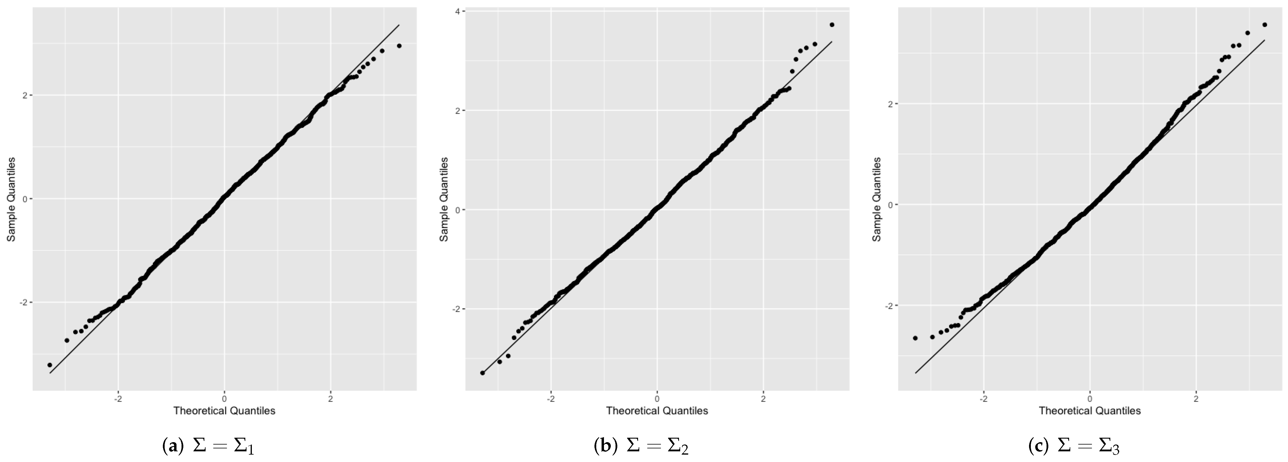
• ${\Sigma }_1={\mathrm{I}}_p$ is the identity matrix.
• ${\Sigma }_2$ is a covariance matrix with ${\sigma }_{i,j}={0.4}^{|i-j|}$.
• ${\Sigma }_3$ is block diagonal matrix, with block $B_{25\times 25}$ in which the diagonal entries are 1 and the off-diagonal entries are 0.15.

${\Sigma }_1$ is for independent cases, while ${\Sigma }_2$ and ${\Sigma }_3$ are for dependent cases.

Theorem 1 shows that $T_{\mathrm{PB}}$ is a linear function of the logarithm of the posterior Bayes factor, which is asymptotically distributed as $N(0,1)$. Q–Q plots are presented in Figure 1 to reveal the asymptotic behavior of $T_{\mathrm{PB}}$ for ${\mu }_1={\mu }_2={\mathbf{0}}_{p\times 1}$ and different choices of $\Sigma$. We can see that points in Figure 1a–c are closely aligned along the identity line, indicating that the distributions of $T_{PB}$ with different $\Sigma$ are close to $N(0,1)$.

We also compare the empirical significance levels and powers of the proposed test with several other tests, including not only tests based on the sum-of-squares-type statistics in [4], referred to as SD, and [7], referred to as CQ, but also a Bayes factor-based test which relies on two random projection approaches as in [12], referred to as RMPBT${}_1$ and RMPBT${}_2$. In this section, the test we proposed is denoted as PB. The results of SD, CQ and RMPBT are cited from [12].

As in [12], we consider two possible alternatives, as follows. Without loss of generality, we shall always take ${\mu }_2={\mathbf{0}}_{p\times 1}$ in the simulations. The proportion of entries of the vector $\delta ={\mu }_1-{\mu }_2$ that are exactly zero is denoted by $p_0$.

• Simulate ${\mu }_1\sim N_p(\mathbf{1},{\mathrm{I}}_p)$, set $p_0$ randomly selected elements to 0, and scale ${\mu }_1$ so that ${\delta }^T{\Sigma }^{-1}\delta =2$.
• Simulate ${\mu }_1\sim N_p(\mathbf{1},{\mathrm{I}}_p)$, set $p_0$ randomly selected elements to 0, and scale ${\mu }_1$ so that $\frac{{\left|\right|\delta \left|\right|}^2}{\sqrt{\mathrm{tr}{\Sigma }^2}}=0.1$.

We take $p_0=0.5,0.75,0.80,0.95,0.975,1$. Note that the case $p_0=1$ corresponds to the null hypothesis and the power becomes the empirical level. A larger $p_0$ corresponds to a more sparse alternative, while a smaller $p_0$ corresponds to a denser one.

For the PB test, we take $m=2p$ and ${\epsilon }_n=1/ln\left(n\right)$. The numerical results are calculated from 1000 replications and summarized in

Table 1. Empirical sizes based on 1000 replications with $\alpha =0.05$, $n_1=n_2=70$ and $p=1000$. RMPBT is the approach of [12], SD is the approach of [4] and CQ is the approach of [7].

	$\mathbf{PB}$	RMPBT${}_1$	RMPBT${}_2$	SD	CQ
${\Sigma }_1$	0.049	0.031	0.030	0.040	0.063
${\Sigma }_2$	0.052	0.038	0.035	0.037	0.049
${\Sigma }_3$	0.060	0.060	0.040	0.045	0.063

,

Table 2. Power analysis of 4 tests assuming the true covariance matrix is $\Sigma ={\Sigma }_1$; $n_1=n_2=70$ and $p=1000$. RMPBT is the approach of [12], SD is the approach of [4] and CQ is the approach of [7].

	${\mathit{p}}_0$	$\mathbf{PB}$	RMPBT${}_1$	RMPBT${}_2$	SD	CQ
Alternative 1	0.975	0.470	0.332	0.309	0.384	0.450
	0.950	0.478	0.388	0.339	0.423	0.474
	0.800	0.482	0.337	0.304	0.389	0.448
	0.750	0.482	0.348	0.294	0.401	0.470
	0.500	0.485	0.372	0.343	0.422	0.473
Alternative 2	0.975	0.764	0.685	0.612	0.722	0.761
	0.950	0.797	0.694	0.612	0.741	0.775
	0.800	0.785	0.660	0.581	0.717	0.762
	0.750	0.806	0.695	0.616	0.756	0.789
	0.500	0.786	0.677	0.588	0.727	0.767

,

Table 3. Power analysis of 4 tests assuming the true covariance matrix is $\Sigma ={\Sigma }_2$. $n_1=n_2=70$ and $p=1000$; RMPBT is the approach of [12], SD is the approach of [4] and CQ is the approach of [7].

	${\mathit{p}}_0$	$\mathbf{PB}$	RMPBT${}_1$	RMPBT${}_2$	SD	CQ
Alternative 1	0.975	0.269	0.259	0.243	0.219	0.266
	0.950	0.277	0.249	0.232	0.209	0.258
	0.800	0.282	0.261	0.222	0.221	0.270
	0.750	0.299	0.264	0.236	0.242	0.284
	0.500	0.336	0.303	0.265	0.268	0.326
Alternative 2	0.975	0.783	0.791	0.738	0.722	0.768
	0.950	0.780	0.786	0.734	0.718	0.766
	0.800	0.794	0.755	0.699	0.700	0.756
	0.750	0.792	0.772	0.722	0.730	0.785
	0.500	0.789	0.753	0.686	0.720	0.766

and

Table 4. Power analysis of 4 tests assuming the true covariance matrix is $\Sigma ={\Sigma }_3$; $n_1=n_2=70$ and $p=1000$. RMPBT is the approach of [12], SD is the approach of [4] and CQ is the approach of [7].

	${\mathit{p}}_0$	$\mathbf{PB}$	RMPBT${}_1$	RMPBT${}_2$	SD	CQ
Alternative 1	0.975	0.296	0.315	0.278	0.245	0.294
	0.950	0.303	0.335	0.307	0.270	0.311
	0.800	0.332	0.348	0.318	0.285	0.343
	0.750	0.357	0.327	0.294	0.278	0.331
	0.500	0.422	0.414	0.379	0.353	0.401
Alternative 2	0.975	0.785	0.836	0.776	0.716	0.755
	0.950	0.801	0.827	0.776	0.730	0.782
	0.800	0.795	0.796	0.734	0.728	0.775
	0.750	0.793	0.790	0.727	0.718	0.764
	0.500	0.778	0.774	0.717	0.720	0.761

. Table 1 compares the empirical sizes of the tests. In general, the test PB performs best in maintaining the significance level. It can be seen that the estimated sizes of PB are reasonably close to the nominal level 0.05. Tests RMPBT and SD show lower empirical levels than the nominal one, whereas test CQ is a little higher.

Table 2, Table 3 and Table 4 compare the powers of the tests. Covariance matrix $\Sigma$ in Table 2, Table 3 and Table 4 are ${\Sigma }_1$, ${\Sigma }_2$ and ${\Sigma }_3$, respectively. Table 2 shows that our test PB substantively outperforms the other three tests for both dense and sparse alternatives. This implies that our method provides the most powerful test compared with the approaches of [4,7,12] for independent cases. In Table 3, the test PB performs better than its competitors in most cases. In Table 4, PB also performs better than the competitors with dense alternatives. Finally, from Table 3 and Table 4, either the prior or the posterior Bayes factor-based tests are better than others. For the dense alternative, the PB test is more powerful than RMPBT.

4. An Application Example

To further explore the practical utility of the posterior Bayes factor-based test, we analyze a real dataset about the small round blue cell tumors (SRBCTs), which is available at https://file.biolab.si/biolab/supp/bi-cancer/projections/info/SRBCT.html, accessed on 1 March 2022.

The SRBCTs are four different childhood tumors including Ewing’s family of tumors (EWS), neuroblastoma (NB), non-Hodgkin lymphoma (BL) and rhabdomyosarcoma (RMS). Our interest is in examining the equality of means of the genes between the EWS and the RMS tumor groups. The dataset contains 29 examples of EWS and 25 examples of RMS with 2038 genes. The observed test statistic of PB is T${}_{PB}=14.19842$ with p-value $\approx 0$, indicating a serious deviation from the null hypothesis.

5. Conclusions

In this article, we explore the potential for the posterior Bayes factor to be a statistic for testing the mean equality of two high dimensional populations. A closed form of the posterior Bayes factor is obtained with simple priors for the model parameters. Asymptotic normality of the posterior Bayes factor is established, and the corresponding test is constructed. Numerical studies and a real-life example show the superiority of the test. Therefore, we recommend the posterior Bayes factor as a test statistic for hypothesis testing in high dimensional settings.

References

- Bai, Z.; Saranadasa, H. Effect of high dimension: By an example of a two sample problem. Stat. Sin. 1996, 6, 311–329. [Google Scholar]
- Hotelling, H. The Generalization of Student’s Ratio. Ann. Math. Stat. 1931, 2, 360–378. [Google Scholar] [CrossRef]
- Anderson, T.W. An Introduction to Multivariate Statistical Analysis; Technical Report; John Wiley & Sons, Inc.: Hoboken, NJ, USA, 1958. [Google Scholar]
- Srivastava, M.S.; Du, M. A test for the mean vector with fewer observations than the dimension. J. Multivar. Anal. 2008, 99, 386–402. [Google Scholar] [CrossRef] [Green Version]
- Srivastava, M.S. A test for the mean vector with fewer observations than the dimension under non-normality. J. Multivar. Anal. 2009, 100, 518–532. [Google Scholar] [CrossRef] [Green Version]
- Srivastava, M.S.; Katayama, S.; Kano, Y. A two sample test in high dimensional data. J. Multivar. Anal. 2013, 114, 349–358. [Google Scholar] [CrossRef]
- Chen, S.X.; Qin, Y.L. A two-sample test for high-dimensional data with applications to gene-set testing. Ann. Stat. 2010, 38, 808–835. [Google Scholar] [CrossRef] [Green Version]
- Feng, L.; Zou, C.; Wang, Z.; Zhu, L. Two-sample Behrens-Fisher problem for high-dimensional data. Stat. Sin. 2015, 25, 1297–1312. [Google Scholar] [CrossRef] [Green Version]
- Cai, T.T.; Liu, W.; Xia, Y. Two-sample test of high dimensional means under dependence. J. R. Stat. Soc. Ser. B Stat. Methodol. 2014, 76, 349–372. [Google Scholar]
- Lopes, M.; Jacob, L.; Wainwright, M.J. A more powerful two-sample test in high dimensions using random projection. Adv. Neural Inf. Process. Syst. 2011, 24, 1206–1214. [Google Scholar]
- Srivastava, R.; Li, P.; Ruppert, D. RAPTT: An exact two-sample test in high dimensions using random projections. J. Comput. Graph. Stat. 2016, 25, 954–970. [Google Scholar] [CrossRef]
- Zoh, R.S.; Sarkar, A.; Carroll, R.J.; Mallick, B.K. A powerful Bayesian test for equality of means in high dimensions. J. Am. Stat. Assoc. 2018, 113, 1733–1741. [Google Scholar] [CrossRef] [PubMed]
- Wang, R.; Xu, X. On two-sample mean tests under spiked covariances. J. Multivar. Anal. 2018, 167, 225–249. [Google Scholar] [CrossRef]
- Kuelbs, J.; Vidyashankar, A.N. Asymptotic inference for high-dimensional data. Ann. Stat. 2010, 38, 836–869. [Google Scholar] [CrossRef] [Green Version]
- Thulin, M. A high-dimensional two-sample test for the mean using random subspaces. Comput. Stat. Data Anal. 2014, 74, 26–38. [Google Scholar] [CrossRef] [Green Version]
- Gregory, K.B.; Carroll, R.J.; Baladandayuthapani, V.; Lahiri, S.N. A two-sample test for equality of means in high dimension. J. Am. Stat. Assoc. 2015, 110, 837–849. [Google Scholar] [CrossRef] [PubMed]
- Yu, W.; Xu, W.; Zhu, L. A combined p-value test for the mean difference of high-dimensional data. Sci. China Math. 2018, 62, 961. [Google Scholar] [CrossRef]
- Chen, S.X.; Li, J.; Zhong, P.S. Two-sample and ANOVA tests for high dimensional means. Ann. Stat. 2019, 47, 1443–1474. [Google Scholar] [CrossRef] [Green Version]
- Zhang, J.T.; Guo, J.; Zhou, B.; Cheng, M.Y. A simple two-sample test in high dimensions based on L2-norm. J. Am. Stat. Assoc. 2020, 115, 1011–1027. [Google Scholar] [CrossRef]
- Zhu, Y.; Bradic, J. Significance testing in non-sparse high-dimensional linear models. Electron. J. Stat. 2018, 12, 3312–3364. [Google Scholar] [CrossRef]
- Aitkin, M. Posterior bayes factors. J. R. Stat. Soc. Ser. B Methodol. 1991, 53, 111–128. [Google Scholar] [CrossRef]
- Wang, R.; Xu, X. Least favorable direction test for multivariate analysis of variance in high dimension. Stat. Sin. 2021, 31, 723–747. [Google Scholar] [CrossRef]
Figure 1.
Quantile–Quantile plot of asymptotic distribution for under the null hypothesis against for different based on 1000 independently generated with , .