
A Spatio-Temporal Graph Neural Network Approach for Traffic Flow Prediction


1
School of Cyber Science and Engineering, College of Information Science and Engineering, XinJiang University, Urmuqi 830046, China
2
School of Computer Science and Engineering, Central South University, Changsha 410075, China
*
Author to whom correspondence should be addressed.
†
These authors contributed equally to this work.
Mathematics 2022, 10(10), 1754; https://0-doi-org.brum.beds.ac.uk/10.3390/math10101754
Submission received: 17 March 2022
/
Revised: 23 April 2022
/
Accepted: 25 April 2022
/
Published: 21 May 2022
Abstract
:The accuracy of short-term traffic flow prediction is one of the important issues in the construction of smart cities, and it is an effective way to solve the problem of traffic congestion. Most previous studies could not effectively mine the potential relationship between the temporal and spatial dimensions of traffic data flow. Due to the large variability in the traffic flow data of road conditions, we analyzed it with “dynamic”, using a dynamic-aware graph neural network model for the hidden relationships between space-time in the deep learning segment. In this paper, we propose a dynamic perceptual graph neural network model for the temporal and spatial hidden relationships of deep learning segments. This model mixes temporal features and spatial features with graphs and expresses them. The temporal features and spatial features are connected to each other to learn potential relationships, so as to more accurately predict the traffic speed in the future time period, we performed experiments on real data sets and compared with some baseline models. The experiments show that the method proposed in this paper has certain advantages.
1. Introduction
Traffic flow prediction is conducive to the mitigation of traffic congestion and the development of smart cities. The improvement of short-time traffic flow prediction accuracy has important implications for travel route planning. Traffic flow prediction is affected by many factors, such as weather, traffic accidents and other unpredictable factors. Better learning about spatiotemporal traffic data relationships is an important factor in predicting accuracy [1]. In recent deep learning based approaches, most of the researchers consider the correlation between temporal and spatial dimensions data separately. Some approaches propose a layered method to learn the data correlation between temporal and spatial dimensions, and then integrate the calculation results of each layer [2,3,4]. In this way, the data correlation of the spatial and temporal dimensions of the traffic data stream may be insufficiently mined [1]. However, graph neural network(GNN) method in the field of deep learning has powerful ability to learn complex data relationships and mine potential features [5,6]. We might be able to closely link the spatiotemporal data of the traffic data stream based on the ability of GNN, and predict the traffic more accurately by learning the value information hidden in it.
In recent years, deep learning methods have been widely used in traffic flow prediction problems. such as Convolutional Neural Network (CNN) [7], Long Short-Term Memory (LSTM) [8], Recurrent Neural Network (RNN) [9,10], deep and embedding learning approach (DELA) [4], deep belief networks (DBN) [11], stacked autoencoder Levenberg–Marquardt [2]. These are the most popular methods in the field of deep learning. They can handle non-linear problems well and deeply mine the previous potential associations of the data. These methods have been widely used in various fields, especially in traffic flow forecasting work. However, Most methods ignore the importance of the spatiotemporal correlation of traffic data. Some methods of spatiotemporal traffic prediction still have insufficient methods for feature selection and extraction of spatiotemporal data [1]. Some methods can only work if the amount of data is large enough [12]. Much work remains to improve the accuracy of predictions. In the past few years, graph neural networks have been widely used and researched. It has strong ability to handle non-linear and deep mining of complex relationships between data. It has excellent performance in text, medicine, image analysis, etc. [5].
This paper proposes a new spatio-temporal relationship learning model. This model aims to mine the hidden relationships of different sections at different time periods, and solves the problem that many models lack the ability to learn spatio-temporal relationships. The model expresses the relationship between road sections as a directed graph. The embedding process of the nodes is divided into two parts, which are the node relationship node embedding and the node embedding of the road sections at different times. The model focuses on studying the spatiotemporal relationship of road sections in different time periods. The effect of the model is tested on multiple real traffic datasets, and other baseline models are compared. The model proposed in this paper shows good prediction results. The second section describes and analyzes the current traffic flow prediction methods, compares the advantages and disadvantages of different methods, and highlights some of the current spatiotemporal graph neural network methods and their shortcomings. The third section describes the detailed process of the proposed method, including the construction of directed graphs, the embedding process of two types of nodes, and the prediction process. The fourth section describes the performance of the proposed method on real data sets, and analyzes the performance between different algorithms. The fourth section summarizes the work of this paper and proposes future research work.The model can be used to study real-time traffic conditions, reasonable road planning, intelligent dispatch of signal lights, real-time analysis of traffic flow, timely prediction of possible traffic accidents, and it can also be used apply to departments that require road data and traffic monitoring. For decades, experts and scholars around the world have developed a variety of short-term traffic flow prediction models using methods from various disciplines, and we have consulted the literature and summarized them, which can be roughly divided into four types of models: predictive models based on intelligence theory, predictive models based on nonlinear theory, predictive models based on linear statistics, and traffic simulation models. In this paper, we mainly study the neural network model of the predictive model based on intelligence theory. At present, there are differences in traffic flow prediction studies at home and abroad. Due to the late start of traffic flow prediction in China, some model algorithms are not very applicable, such as people using regression method and speed density traffic flow model to predict traffic conditions. This method has the advantages of flow rate linear regression maturity, simple detection equipment, small size and reasonable price; But its drawbacks are also very obvious, mainly in real time.
2. Related Work
Traffic flow prediction can effectively deal with the problem of traffic congestion. Traffic flow prediction is closely related to time series and the spatial distribution of roads. It processes a large amount of traffic data and analyzes the potential correlation between complex traffic environment data. The traffic prediction model will use the collected historical traffic flow data as input data, and process the model to output future traffic flow. Such models include differential integrated moving average autoregressive model (ARIMA) [13], k-Nearest Neighbor algorithm (k-NN) [14], Multilayer Perceptron (MLP) [15], Neural Network Model and Kalman filter (KF) [16]. It is not difficult to see from many literatures that there are currently a variety of algorithms applied to intelligent traffic flow prediction problems. These methods can be roughly divided into three types of methods: model statistics, traditional machine learning, and deep learning, and deep learning methods. Model statistical methods include multiple linear regression methods, exponential smoothing methods, and differential integrated moving average autoregressive models. Machine learning methods include k-nearest neighbor algorithm (k-nn) [14], Markov [17], and artificial neural network (ANN) [18]. Wu and at all proposed a new traffic flow prediction model Based on GNN, Bi-GRCN, which combines GCN and Bi-GRU. By using real traffic data and comparing Bi-GRCN with other neural network models and traditional traffic prediction methods. They came to experimental conclusions; compared to GCN and GRU, Bi-GRCN has higher accuracy and better traffic prediction performance. Bi-GRCN is also more effective than traditional traffic prediction methods HA, ARIMA and SVR [19]. Jiang and his colleagues present an effective multi-step traffic prediction model, ABSTGCN-EF, which combines GCN and AEN. They added a meaningful time slot notation mechanism to the model. The results show that the model ABSTGCN-EF has great potential in exploring the structure of space-time, and at the same time, it also has better modeling capabilities and may have stable performance in longer prediction tasks [20]. Zakarya also proposed a novel deep spatiotemporal neural network model DHSTNet, and the DHSTNet model they proposed considered LSTM and CNN models to achieve the advantages of spatiotemporal features. They also benefited from GCN-DHSTNet, which further developed a graph convolutional network that allowed it to capture both spatio-temporal features as well as external branches. By comparing two real-world traffic datasets, we can see the superiority of the GCN-DHSTNet model over the most advanced models available [21].
3. Statistical Methods
In the early days of traffic flow prediction, statistical models dominated, and the method was usually based on the assumption of specific functions for certain variables. These methods are simple and efficient, and can predict the distribution and cycle information of traffic flow data. However, the prediction of traffic flow is affected by multiple factors, and simple statistical models cannot deeply dig the potential relationships between various aspects of data, leading to problems such as insufficient prediction accuracy. The representative statistical model methods include differential integrated moving average autoregressive model (ARIMA) [13], exponential smoothing method, Holt-Winter [22] method and other improved methods Dantas et al. [23], Abadi et al. [24], Williams and Hoel [25]. When analyzing historical data such as traffic flow, traffic speed, and travel time based on statistical model construction methods, many assumptions are often proposed. These assumptions are generally based on the existing characteristics of historical data, and historical traffic data are also given to future traffic data. Data characteristics: for example: traffic rate, weather conditions, and road congestion in historical time, but this type of method does not take into account changes caused by future weather conditions, road visibility, and traffic accidents.
3.1. Traditional Machine Learning Methods
Machine learning methods can be roughly divided into supervised learning, unsupervised learning, etc. Supervised learning has feature and label, even if the data are unlabeled, it can also be determined by learning the relationship between features and labels, and it can generate a function to map the input to the appropriate output through the correspondence between the existing part of the input data and the output data.In contrast, unsupervised learning has only features, no labels, and it divides data into several classes (clusters) through their intrinsic connections and similarities. At the same time, it can also learn some characteristics from the data according to a certain measure according to the characteristics of the data itself. Widely used supervised learning techniques include ANN [26], Support Vector Machines (SVM) [27], Bayesian Methods [28], and k-Nearest Neighbors (k-NN) [29], while popular unsupervised learning techniques include k-means [30], autoencoder [31], principal component analysis (PCA) [32], DBN [11] For each data set, a set of attributes called features will be extracted as input to the ML model. In addition, if the data has high dimensionality, it is difficult to extract the correct features. Similarly, feature evaluation and extraction based on manually labeled data is also a time-consuming task. According to the above research, traffic flow prediction technology can be roughly divided into: parametric algorithm and non-parametric algorithm.
Parametric algorithms (model-based algorithms) consist of a fixed number of parameters that are based on certain assumptions about the format of the data. The parameter algorithms that make static assumptions greatly reduce the computational difficulty and complex traffic data relationships. In addition, uncertainty, so it does not apply to traffic datasets. In contrast, non-parametric algorithms are not constrained by various assumed parameters. In these algorithms, the data are not assumed to follow any distribution or model. While the parametric approach is useful when observed traffic patterns change regularly, errors are expected in the presence of periodic variations and irregular noise. Therefore, nonparametric methods are more popular in forecasting due to the presence of complex and nonlinear patterns in traffic flows. Popular nonparametric methods include models such as SVM, SVR, wavelet analysis, ANN, DL, and time series models, with KF and linear regression being typical parametric methods. In addition, Bayesian networks can be used to process traffic flow data because of its variability and the ability to calculate predicted averages quickly. In addition, the model can update predictions when new data are available. Bayesian networks enable a probability distribution between the input and output of traffic flow data. The authors in [33] designed a Bayesian model that uses spatial historical traffic data from adjacent road links to predict traffic flow in road segments. In addition, in order to add spatiotemporal information, the authors in [34] designed Bayesian networks by using Pearson correlation coefficients to select input variables. In addition, refs. [35,36,37] have used Bayesian networks for traffic flow prediction [19].
3.2. Deep Learning Methods
Artificial neural networks have been served as a powerful method for mathematical modeling of traffic data. The capabilities provided by artificial neural networks include self-learning, self-organization, and pattern recognition. They can also perform nonlinear approximation learning between input and output spaces. As nonparametric methods, they do not make any type of assumptions about the distribution of the data. In addition, the parallel structure of artificial neural networks makes their implementation on parallel computers very efficient. In the unsupervised DL algorithm, it was found that the DBN model can extract random features without the need to manually extract features. The author [38] use DBNs to learn robustness and nonlinearity from flow-in data. This paper proposes a two-layer deep learning model that combines the regression layer at the top with the DBN at the bottom. This approach supports Multitasking Learning (MTL), where different tasks are integrated and models are trained together. To get better predictions, MTL uses the idea of weight sharing in DBN [39]. Here, the sigmoidal regression function is used at the top to perform supervised fine-tuning. Experiments show that the overall performance can be improved by the MTL scheme. Similarly, for experimental authors, DBNs with different depths and number of nodes were used. In addition, the author in [40] proposed a DBN-based traffic flow prediction model. A variant of The Demoster-Shafer evidence theory that uses The Demoster conditional rules, combines predictive beliefs in data history structures with anomalous event data modules. Here, the supervised BP algorithm is used to implement multitasking learning. In addition, due to the dynamic nature of traffic data, traffic flow does not always follow the same pattern throughout the day. For example, the density of traffic during the day is greater than the density of traffic at night. In this case, ref. [41] Zhang et al. genetic algorithm was used to extract the optimal hyperparameters of DBN at different time intervals. In addition, the authors in [42] discussed the effects of pre-training with different DBNs.
4. Methodology
As the problem of traffic forecasting is getting more and more attention and a large amount of hardware for traffic data collection is currently being invested in traffic monitoring, the amount of traffic data continues to increase. We need efficient computing models for analyzing traffic data. At present, there are many models for analyzing and predicting traffic flow. GraphSAGE is a model that uses neighbor node aggregation to efficiently learn nodes. It has good computational efficiency and command in classification problems, system recommendations, and drug detection. Satisfactory performance. However, the data objects it processes mainly have non-time series and strong order characteristics. Traffic flow data has strong time series characteristics, and the potential relationship between time and space is more complicated. Therefore, GraphSAGE cannot handle such problems well. This paper proposes a new type of spatio-temporal graph neural network for learning and predicting traffic flow. This model borrows the idea of the GraphSAGE model and constructs a directed graph to represent the spatio-temporal relationship between routes. Skip-gram [43] method to perform unsupervised learning on a certain road segment to predict the traffic situation at the future moment. The innovation of this model is that Graph SAGE is an inductive graph learning model that first samples nodes, then aggregates adjacent information, and finally processes the final task (such as node classification). Different from the general matrix decomposition-based graph embedding method, Graph SAGE uses the characteristics of nodes (such as text, node degree, node attribute description, etc.) to learn the node embedding pattern (i.e., function, etc.), rather than directly learning the final node embedding, so it can use a good learning node embedding mode to deal with unseen nodes and even see new graph structures.
4.1. The Define of STGNN
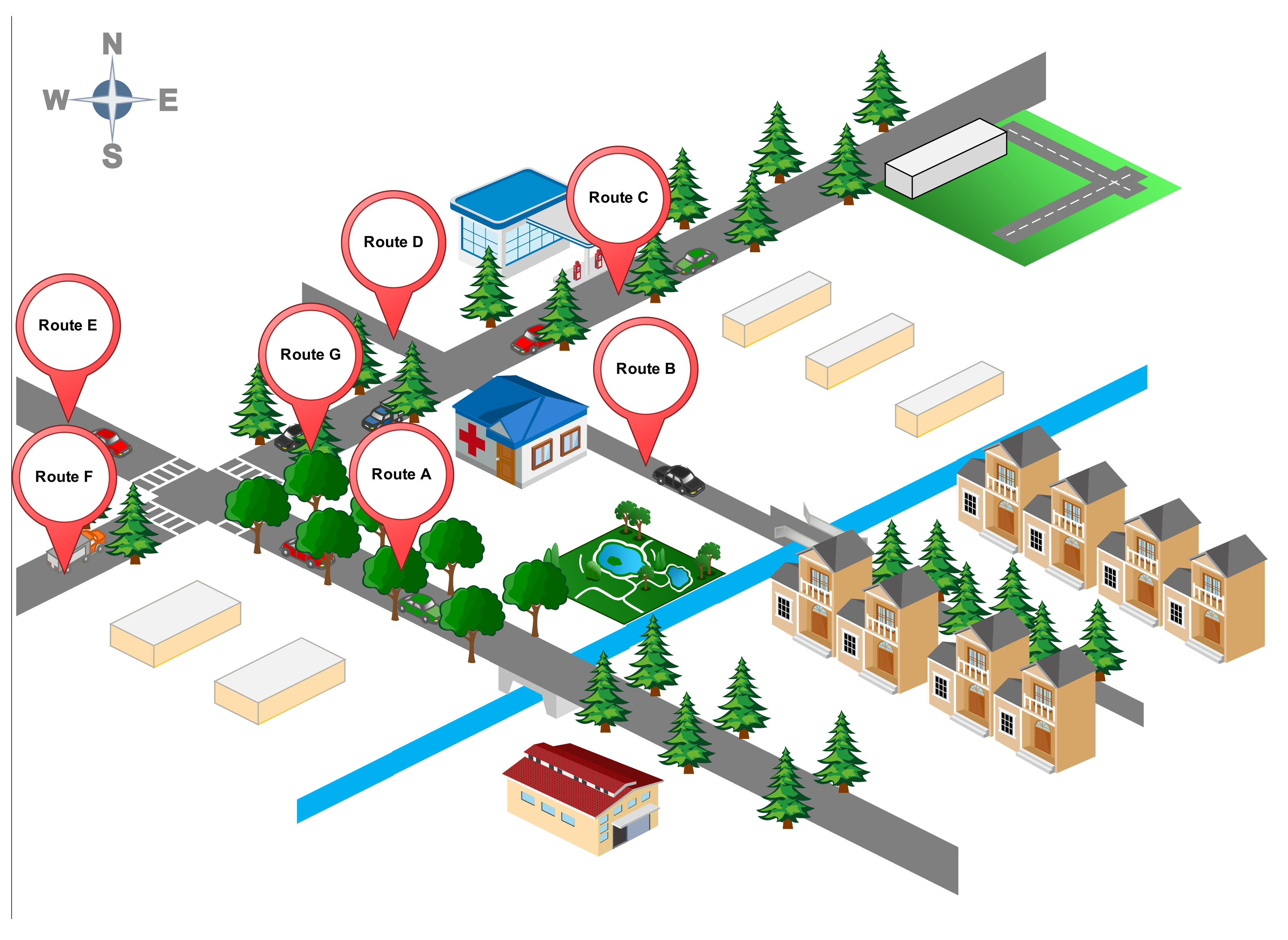
STGNN’s name is “Space And Time Graph Neural Network”. STGNN is a spatiotemporal GNN framework specifically designed to model a series of data with complex topologies and time dependencies. This paper mainly predicts the traffic flow under complex road conditions and studies the spatio-temporal relationship between roads. The road variants included in Figure 1 are complex and substantially consistent with most complex road conditions, so they can provide a reasonable and effective premise for the research in this paper. We transform the road structure into a structure represented by a undirected graph, and turn the problem of predicting road traffic flow into a problem of learning the correlation between nodes in the graph. We focus on learning the implicit information about the changes in traffic flow between different sections of the road at different times. We can predict the traffic flow situation in the future time period based on the historical traffic data changes of the road sections and the implicit relationship between the road sections. As shown in Figure 1, it is an example of road structure. We divide all roads into 7 sections, named Route A, Route B, Route C, Route D, Route E, Route F, and Route G. It contains two crossroads, one of which has a sidewalk. Route C, F and G are from the same straight road. Route B and D can form a straight road. Route A and E are on the same road. Route C, B, D and G can communicate with each other route. There is a complex relationship between routes, which affect each other. In addition, the degree of influence between the lines is slight, such as the effect between route B and route F is less than route F and route G. We can observe that route B and F are more closely related, while route F and G are more alienated.
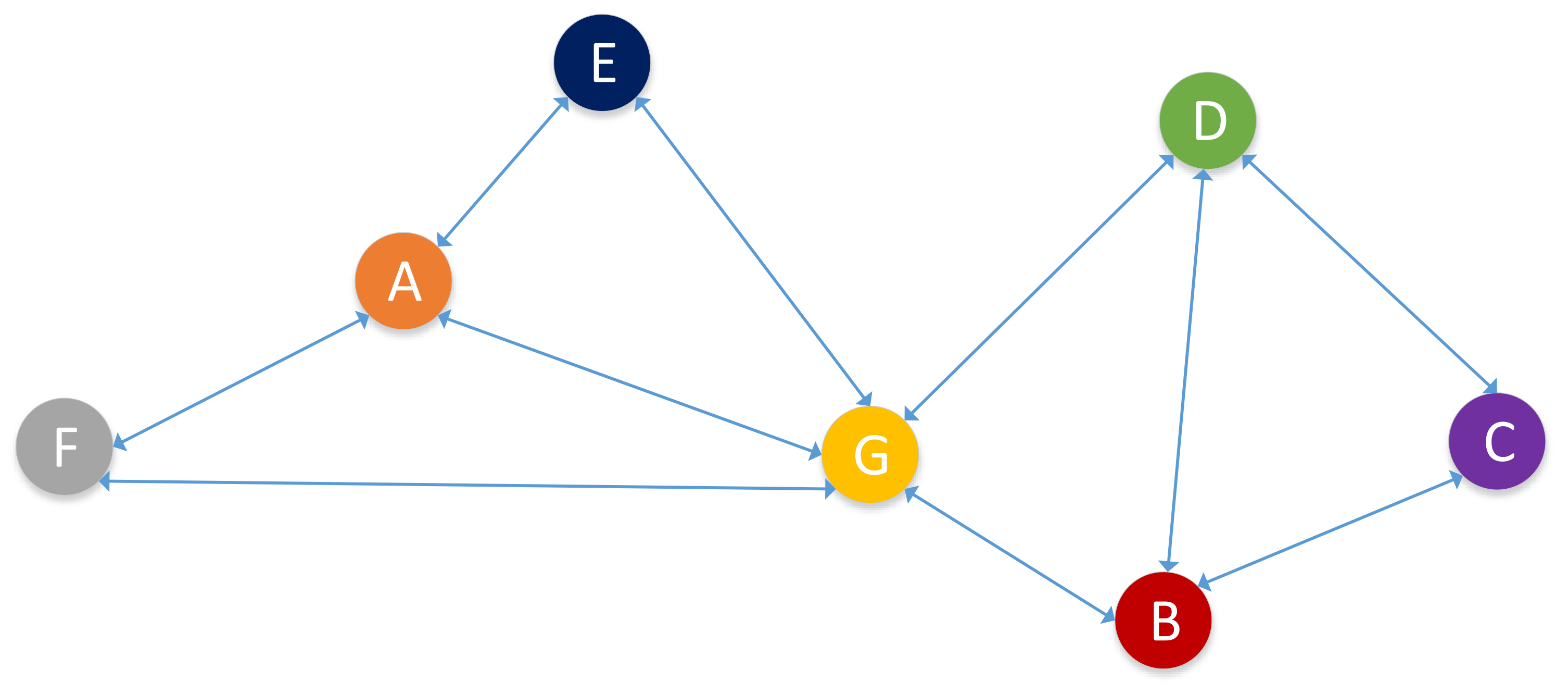
As shown in Figure 2, We represent road relationships as graph relationships, with all alignments as corresponding nodes in the graph, all the routes as the corresponding nodes in the graph, and the connectivity between the routes as the lines between the nodes in the directed graph. We can express the road structure by the following rules:
where R denotes the whole road structure, N denotes the all the routes, denotes the start location of the route, denotes the end location of the route. In addition, N contains two types of nodes, one is the the embedding node of the route, another one is the embedded representation of the same route at different time periods.
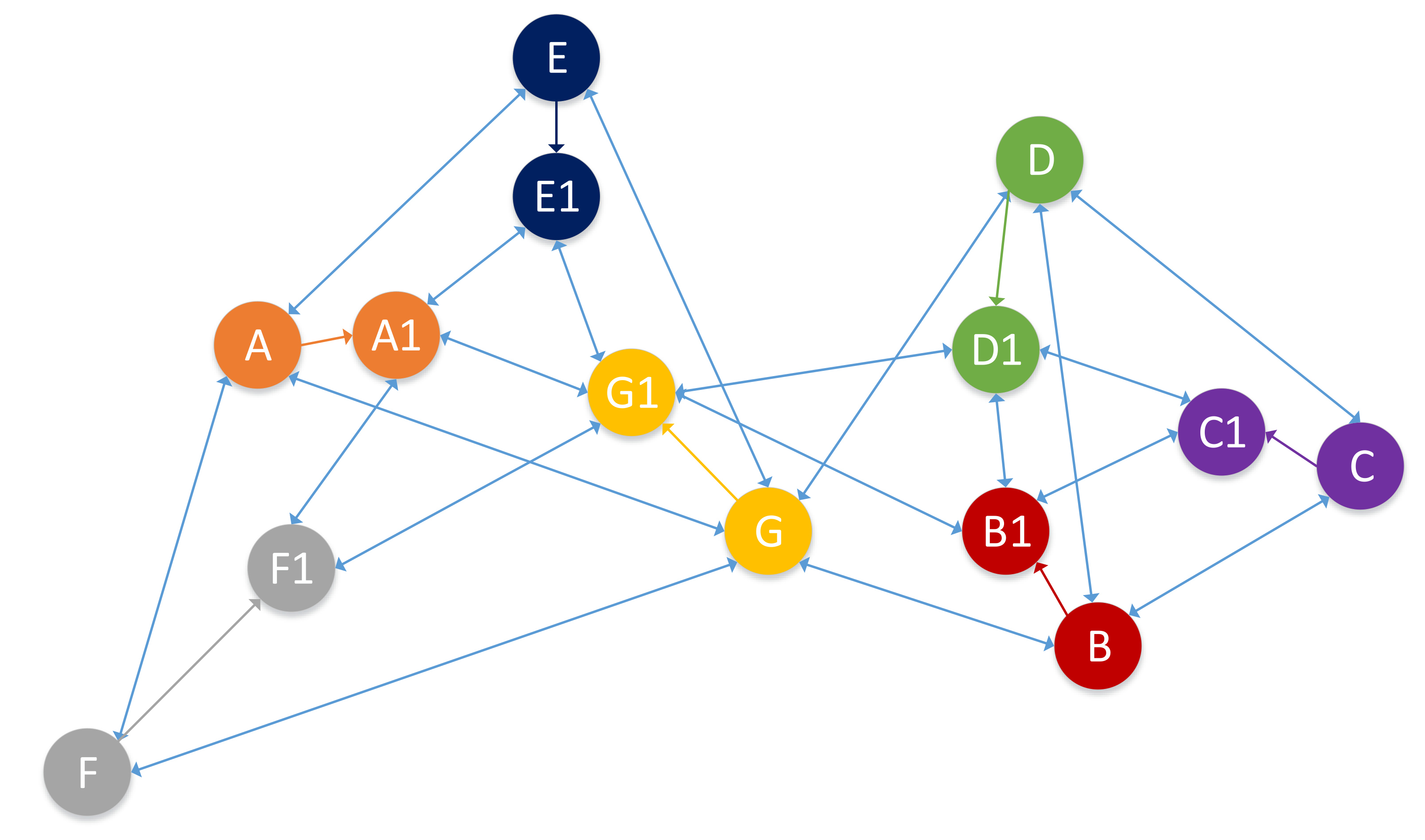
As shown in Figure 3, it describes the spatio-temporal relationship of road sections. The node E1 represents the embedded representation of route E in a certain time. Furthermore, E and E1 both interact with each other and update features. Similarly, this way also works for G and G1, A and A1, etc. We can use the following equation to represent the relationship between nodes:
where denotes the spatio-temporal directly graph, R can be known from the Equation , contains embedded representation of the routes at different time periods, the nodes are denoted as , such as E1, A1, G1, D1 and so on. Nodes in the same time period can be connected in both directions. Nodes in different time periods cannot be connected or can only be unidirectional. denotes the start node of , denotes the end node of . We can observe that E1 and A1, E and A are all connected in both directions, but E1 and A cannot be directly connected. N and have the same structure.
As shown in Figure 3, we can define , . We can observe that , it means A is the start node and is the end node when . Similarly, , and . In addition, we can find that , , and . But, we can observe that is not connected to E, it is expressed as . Others related to are denoted as , .
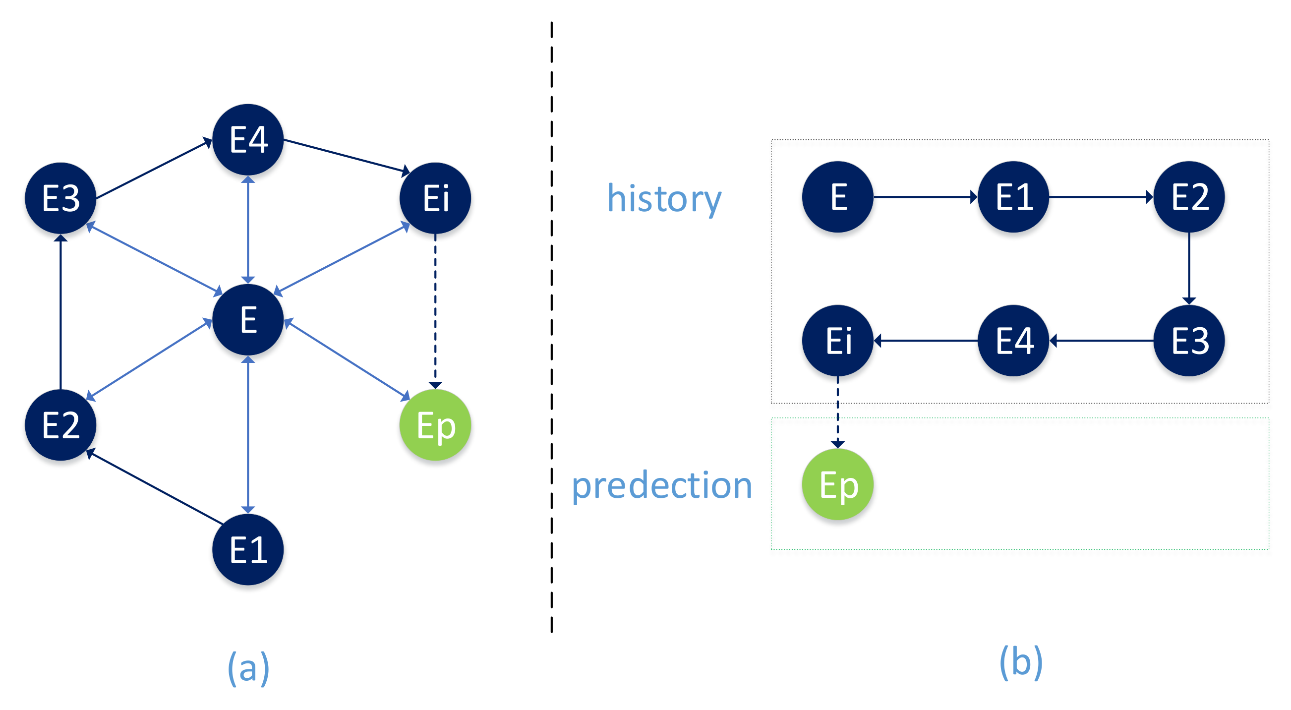
Next, we can observe from Figure 4 that the E node and the road segment E are represented at different time periods and the relationship between the nodes at different time periods. is the embedding of road segment E at time , we denote this as follow:
where denotes a time period, is the traffic flow features of route N, the value of is different between and , is the embedding vector, F denotes the node embedding vector for all time periods. Although and have the same value, and is different. From Equation , we know that , , , , and are denoted the route E embeddding during different time periods. Especially, is the node that denoted in the future time period.
4.2. The Prediction Process of STGNN
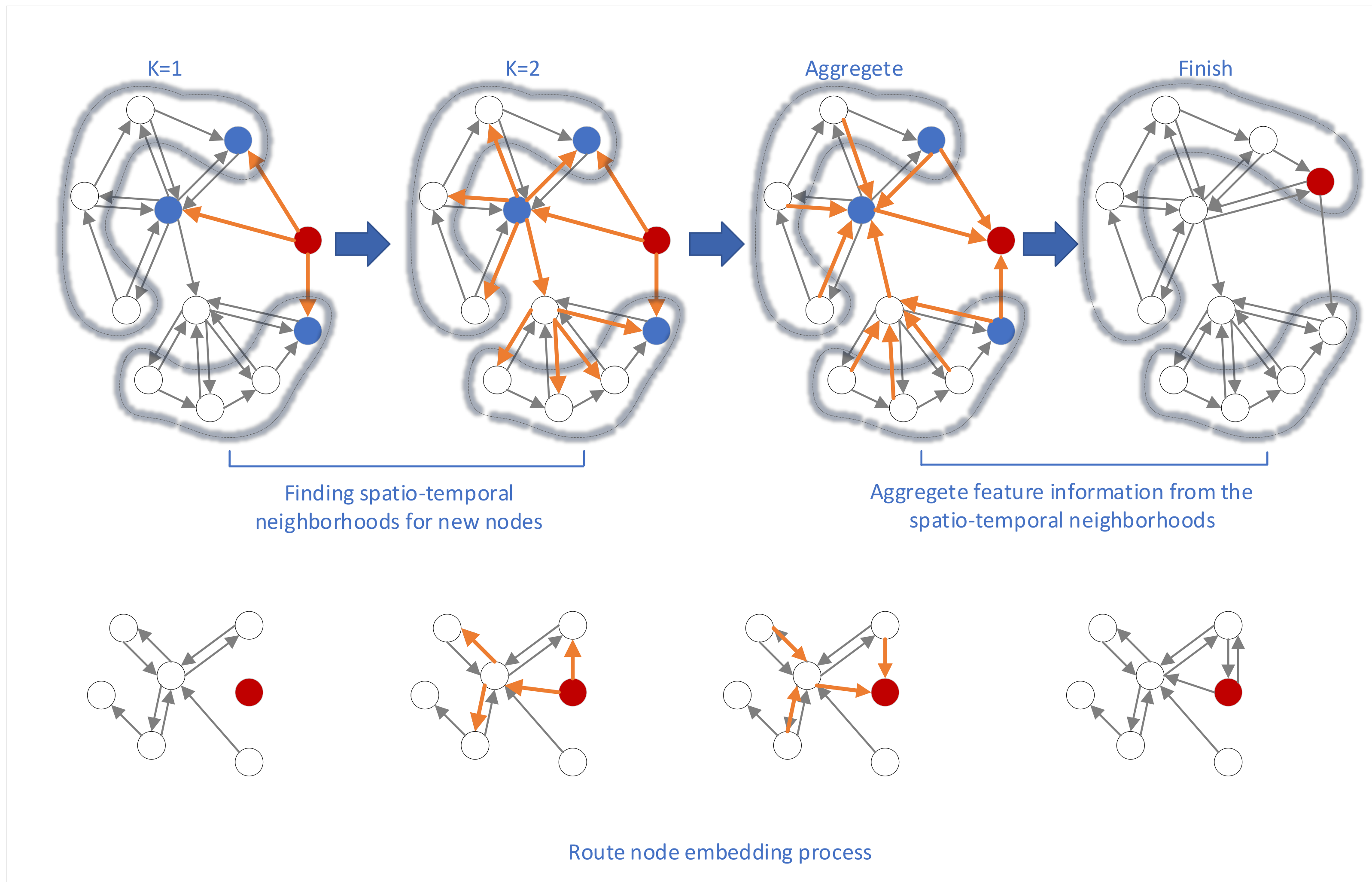
As shown in Figure 5, the spatio-temporal graph neural network mainly includes two types of node embeddings: the node embedding of the directed graph initialization of the relationship between the original road segments and the traffic flow node embedding of the road segments at different times.
The initialization process of constructing a multi-segment segment as a directed graph is also the embedding process of the segment node. First, find the connectable neighbors of the new node A. The range of the neighbors is controlled by the value of k. When k = 1, the nearest effective neighbor to A is selected. These neighbor nodes also have their own neighbor nodes, and then select the effective neighbor nodes of node A’s neighbor nodes when k = 2, and can freely control the value of k as needed, and finally perform an aggregation operation on all selected nodes to obtain the characterization of node A information.
The traffic flow of the road section at different times can be represented by different nodes. Assume that node Ati represents the state of node A at time . is only related to the node of , and is directly related to node A. Set k = 1. When the node needs to be embedded, first find if there are any other nodes in the time period at . If there is a node connected to the node, select its neighbor node. Similarly, set k = 2 as needed, and then find the neighbor nodes of the selected neighbor nodes, and so on. Finally, ’s representation vector is obtained based on the aggregation of these neighbor nodes.
5. Experiments
5.1. Datesets Details
In this section we use two real datasets to verify the validity of the STGNN model. They are METR-LA and PEMS-BAY. METR-LA is the data collected by the monitors on the Highway of Los Angeles County. Here we use the data of 207 sensors and select the data from 1 March 2012 to 30 June 2016 as our experimental data [44,45]; PEMS-BAY is from California Transportation Agencies. The data of 325 sensors in this data set is from 1 January 2017 to 31 May 2017. We aggregate the readings of the two traffic data in 5 min units and use the Z-Score method to normalize the data. We also select 70% of data for training, 20% of data for testing, and the remaining 10% of data for verification [45]. In order to obtain the attributes of the length of the segment between the sensors, we use the thresholded Gaussian Kernel Method to build the adjacency matrix [45]. The calculation formula is shown below:
In our experiments, we set , if , we set , denotes the weight of the road from to , denotes the distance from sensor to sensor .
5.2. Comparison Models
We have selected several classic models to compare the performance of the models proposed in this paper. These models are Historical Average (HA), Auto-Regressive Integrated Moving Average model with Kalman filter (), Support Vector Regression (SVR) [46], Feed forward Neural network (FNN), Recurrent Neural Network with fully connected LSTM hidden units (FC-LSTM) [47].
5.3. Evaluation Indicators
We selected three classic evaluation indicators to evaluate the performance of the model. We assume that represents real data and represents predicted data, and n denotes the indices of samples, These indicators are as follows,
- RMSE: Root Mean Square Error
- MAPE: Mean Absolute Percentage Error
- MAE Mean Absolute Error
5.4. Performance Comparison
As shown in Table 1 and Table 2, We divide the data set METR-LA according to three time intervals, which are 15 min, 30 min and 60 min. Many models are used to test on different division methods, and the test results are evaluated using three evaluation indicators: MAE, RMSE, and MAPE. Table 1 lists the data of the model test results. It can be seen that the STGNN model proposed in this paper has the smallest values on different evaluation indicators in different time periods, indicating that the effect of the model is optimal, followed by the DCRNN method. In the same way, we tested the performance of each model on the dataset PEMS-BAY. The STGNN proposed in this paper performs best among multiple comparison objects.
From the data in Table 1 and Table 2, we can find that as the partitioning time interval increases, the performance of all models except the HA method decreases. The performance of all models concerned in this paper on the data set PEMS-BAY is better than that on the data set METR-LA. All methods have more obvious changes in the MAPE index of the two datasets.
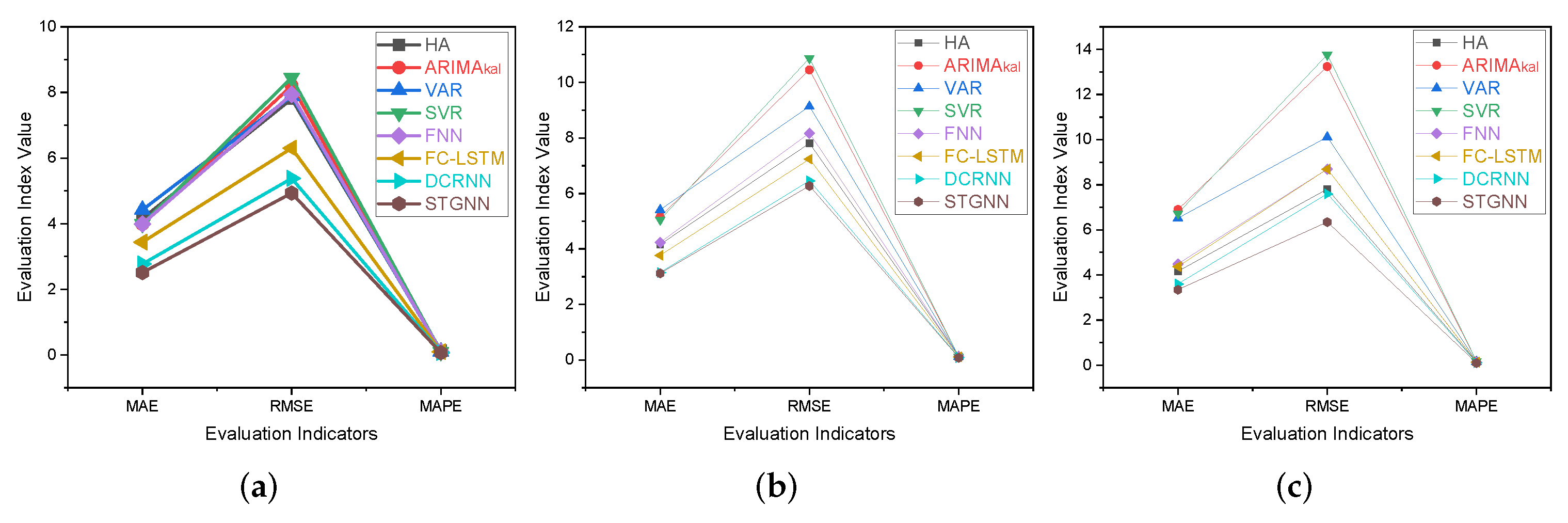
As shown in Figure 6, we can observe the performance comparison of models over different time periods on the METR-LA datasets, (a) shows the performance comparison of multiple algorithms on 15 min time division. Similarly, (b) shows the performance on 30 min time period, (c) denotes the effect on 1 hour time period. We can observe from (a) that the performance of HA, , FNN and VAR are similar, these methods is far worse than FC-LSTM. DCRNN is better than FC-LSTM, STGNN is the best one. From (b), we can find that the performance of HA and are similar. In addition, DCRNN and STGNN are also similar, and STGNN is better than DCRNN on these three evaluation indicators. SVR and have the worst performance, STGNN and DCRNN are the best, and the performance of other methods is centered.
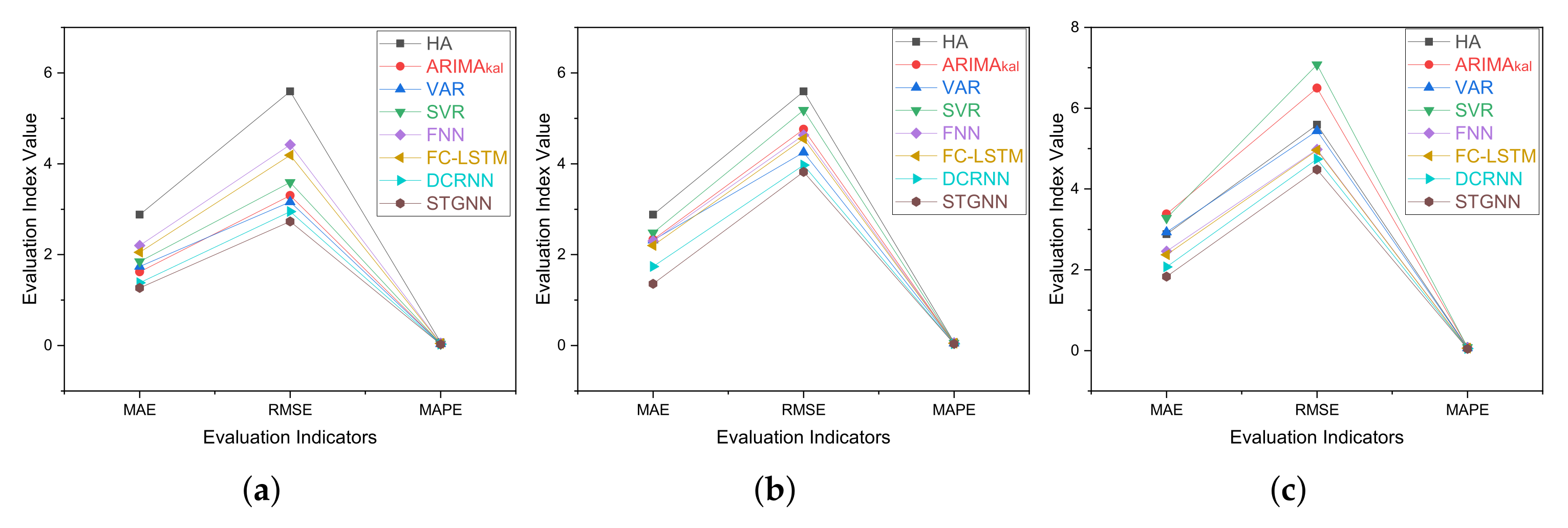
As shown in Figure 7, it shows the performance of the model on the PEMS-BAY dataset. From (a), we can observe that the value of SVR, , VAR, DCRNN and STGNN is similar, and STGNN is the best method. The method other than HA has a small gap in the evaluation index MAE. From (b) and (c), STGNN is the best method in the evaluation MAE, RMSE and MAPE, the second one is DCRNN.
As shown in Figure 6 and Figure 7, we can conclude that the performance of the STGNN method is the best of all reference methods, followed by the DCRNN method. With the increase of time interval division of multiple methods, the ranking of performance becomes unstable, such as the FC-LSTM method. However, the ranking of the STGNN and DCRNN methods is not affected by these factors, and the STGNN method has shown superior results in experiments.
6. Conclusions
This paper mainly studies the potential relationship between traffic speed and space, improves the accuracy of traffic speed prediction, and achieves accurate prediction and solves the increasing road traffic pressure, increasing traffic accidents and traffic congestion problems in urban development. This paper focuses on the potential relationship between space-time of road sections. To this end, we propose a space-time graph neural network model for deep learning and mining the spatio-temporal implicit relationship of road sections. The model compares spatiotemporal features and expresses graphs, connecting temporal and spatial features to understand potential relationships to more accurately predict the speed of traffic at future times. To more accurately predict the speed of traffic in future time periods, we conducted experiments on real datasets and compared them with some baseline models. Experiments show that this method has a novel graph neural network layer with a location attention mechanism that can better aggregate traffic flow information from adjacent roads. However, for some reason, the experimental data were not updated in a timely manner. In future research work, we will be more inclined to improve the ability of the model to resist noise interference, such as rainy days and traffic accidents, and continuously improve and update experimental data to ensure the accuracy of data and conclusions.
Author Contributions
Conceptualization, Y.L.; methodology, H.F. and Y.L.; software, H.F.; validation, Y.L. and H.F.; formal analysis, H.F. and Y.L.; investigation, Y.L.; resources, H.F. and Y.L.; data curation, H.F. and W.Z.; writing—original draft preparation, H.F.; writing—review and editing, H.F. and Y.L.; visualization, H.F. and W.Z.; supervision, Y.L.; project administration, Y.L. and W.Z.; funding acquisition, Y.L. and W.Z. All authors have read and agreed to the published version of the manuscript.
Funding
This work was supported in part by the National Natural Science Foundation of China under Grant U1911401 and the National Natural Science Foundation of China under Grant U1435215.
Institutional Review Board Statement
Not applicable.
Informed Consent Statement
Not applicable.
Data Availability Statement
Not applicable.
Conflicts of Interest
The authors declare no conflict of interest.
References
- Pavlyuk, D. Feature selection and extraction in spatiotemporal traffic forecasting: A systematic literature review. Eur. Transp. Res. Rev. 2019, 11, 6. [Google Scholar] [CrossRef]
- Yang, H.F.; Dillon, T.S.; Chen, Y.P.P. Optimized structure of the traffic flow forecasting model with a deep learning approach. IEEE Trans. Neural Netw. Learn. Syst. 2016, 28, 2371–2381. [Google Scholar] [CrossRef] [PubMed]
- Alsolami, B.; Mehmood, R.; Albeshri, A. Hybrid Statistical and Machine Learning Methods for Road Traffic Prediction: A Review and Tutorial. In Smart Infrastructure and Applications; Springer: New York, NY, USA, 2020; pp. 115–133. [Google Scholar]
- Zheng, Z.; Yang, Y.; Liu, J.; Dai, H.N.; Zhang, Y. Deep and Embedded Learning Approach for Traffic Flow Prediction in Urban Informatics. IEEE Trans. Intell. Transp. Syst. 2019, 20, 3927–3939. [Google Scholar] [CrossRef]
- Wu, Z.; Pan, S.; Chen, F.; Long, G.; Zhang, C.; Yu, P.S. A comprehensive survey on graph neural networks. arXiv 2019, arXiv:1901.00596. [Google Scholar] [CrossRef] [PubMed] [Green Version]
- Zhou, J.; Cui, G.; Zhang, Z.; Yang, C.; Liu, Z.; Wang, L.; Li, C.; Sun, M. Graph neural networks: A review of methods and applications. arXiv 2018, arXiv:1812.08434. [Google Scholar] [CrossRef]
- Ma, X.; Dai, Z.; He, Z.; Ma, J.; Wang, Y.; Wang, Y. Learning traffic as images: A deep convolutional neural network for large-scale transportation network speed prediction. Sensors 2017, 17, 818. [Google Scholar] [CrossRef] [Green Version]
- Gers, F.A.; Schmidhuber, J.; Cummins, F. Learning to forget: Continual prediction with LSTM. Neural Comput. 1999, 12, 2451–2471. [Google Scholar] [CrossRef]
- Gao, Y.; Er, M.J. NARMAX time series model prediction: Feedforward and recurrent fuzzy neural network approaches. Fuzzy Sets Syst. 2005, 150, 331–350. [Google Scholar] [CrossRef]
- Van Lint, J.; Hoogendoorn, S.; van Zuylen, H.J. Freeway travel time prediction with state-space neural networks: Modeling state-space dynamics with recurrent neural networks. Transp. Res. Rec. 2002, 1811, 30–39. [Google Scholar] [CrossRef]
- Hinton, G.E. Deep belief networks. Scholarpedia 2009, 4, 5947. [Google Scholar] [CrossRef]
- Moussavi-Khalkhali, A.; Jamshidi, M. Feature Fusion Models for Deep Autoencoders: Application to Traffic Flow Prediction. Appl. Artif. Intell. 2019, 33, 1179–1198. [Google Scholar] [CrossRef]
- Yu, G.; Zhang, C. Switching ARIMA model based forecasting for traffic flow. In Proceedings of the 2004 IEEE International Conference on Acoustics, Speech, and Signal Processing, IEEE, Montreal, QC, Canada, 17–21 May 2004; Volume 2, pp. ii–429. [Google Scholar]
- Yu, B.; Song, X.; Guan, F.; Yang, Z.; Yao, B. k-Nearest neighbor model for multiple-time-step prediction of short-term traffic condition. J. Transp. Eng. 2016, 142, 04016018. [Google Scholar] [CrossRef]
- Innamaa, S. Short-term prediction of traffic situation using MLP-neural networks. In Proceedings of the 7th World Congress on Intelligent Transport Systems, Turin, Italy, 6–9 November 2000; pp. 6–9. [Google Scholar]
- Guo, J.; Huang, W.; Williams, B.M. Adaptive Kalman filter approach for stochastic short-term traffic flow rate prediction and uncertainty quantification. Transp. Res. Part C Emerg. Technol. 2014, 43, 50–64. [Google Scholar] [CrossRef]
- Ko, E.; Ahn, J.; Kim, E. 3D Markov process for traffic flow prediction in real-time. Sensors 2016, 16, 147. [Google Scholar] [CrossRef] [Green Version]
- Smith, B.L.; Demetsky, M.J. Short-term traffic flow prediction models—A comparison of neural network and nonparametric regression approaches. In Proceedings of the IEEE International Conference on Systems, Man and Cybernetics, San Antonio, TX, USA, 2–5 October 1994; Volume 2, pp. 1706–1709. [Google Scholar]
- Jiang, W.; Xiao, Y.; Liu, Y.; Liu, Q.; Li, Z. Bi-GRCN: A Spatio-Temporal Traffic Flow Prediction Model Based on Graph Neural Network. J. Adv. Transp. 2022, 2022, 5221362. [Google Scholar] [CrossRef]
- Ye, J.; Xue, S.; Jiang, A. Attention-based spatio-temporal graph convolutional network considering external factors for multi-step traffic flow prediction. Digit. Commun. Netw. 2021. [Google Scholar] [CrossRef]
- Ali, A.; Zhu, Y.; Zakarya, M. Exploiting dynamic spatio-temporal graph convolutional neural networks for citywide traffic flows prediction. Neural Netw. 2022, 145, 233–247. [Google Scholar] [CrossRef]
- Grubb, H.; Mason, A. Long lead-time forecasting of UK air passengers by Holt–Winters methods with damped trend. Int. J. Forecast. 2001, 17, 71–82. [Google Scholar] [CrossRef]
- Dantas, T.M.; Oliveira, F.L.C.; Repolho, H.M.V. Air transportation demand forecast through Bagging Holt Winters methods. J. Air Transp. Manag. 2017, 59, 116–123. [Google Scholar] [CrossRef]
- Abadi, A.; Rajabioun, T.; Ioannou, P.A. Traffic flow prediction for road transportation networks with limited traffic data. IEEE Trans. Intell. Transp. Syst. 2014, 16, 653–662. [Google Scholar] [CrossRef]
- Williams, B.M.; Hoel, L.A. Modeling and forecasting vehicular traffic flow as a seasonal ARIMA process: Theoretical basis and empirical results. J. Transp. Eng. 2003, 129, 664–672. [Google Scholar] [CrossRef] [Green Version]
- Patterson, D.W. Artificial Neural Networks: Theory and Applications; Prentice Hall PTR: Hoboken, NJ, USA, 1998. [Google Scholar]
- Cortes, C.; Vapnik, V. Support-vector networks. Mach. Learn. 1995, 20, 273–297. [Google Scholar] [CrossRef]
- Heckerman, D. A tutorial on learning with Bayesian networks. In Innovations in Bayesian Networks; Springer: Berlin, Germany, 2008; pp. 33–82. [Google Scholar]
- Keller, J.M.; Gray, M.R.; Givens, J.A. A fuzzy k-nearest neighbor algorithm. IEEE Trans. Syst. Man Cybern. 1985, 4, 580–585. [Google Scholar] [CrossRef]
- MacQueen, J. Some methods for classification and analysis of multivariate observations. In Proceedings of the Fifth Berkeley Symposium on Mathematical Statistics and Probability, Oakland, CA, USA, 1 January 1967; Volume 1, pp. 281–297. [Google Scholar]
- Liou, C.Y.; Cheng, W.C.; Liou, J.W.; Liou, D.R. Autoencoder for words. Neurocomputing 2014, 139, 84–96. [Google Scholar] [CrossRef]
- Pearson, K. LIII. On lines and planes of closest fit to systems of points in space. Lond. Edinb. Dublin Philos. Mag. J. Sci. 1901, 2, 559–572. [Google Scholar] [CrossRef] [Green Version]
- Sun, S.; Zhang, C.; Yu, G. A Bayesian network approach to traffic flow forecasting. IEEE Trans. Intell. Transp. Syst. 2006, 7, 124–132. [Google Scholar] [CrossRef]
- Sun, S.; Zhang, C.; Zhang, Y. Traffic flow forecasting using a spatio-temporal bayesian network predictor. In Proceedings of the International Conference on Artificial Neural Networks, Warsaw, Poland, 11–15 September 2005; Springer: New York, NY, USA, 2005; pp. 273–278. [Google Scholar]
- Castillo, E.; Menéndez, J.M.; Sánchez-Cambronero, S. Predicting traffic flow using Bayesian networks. Transp. Res. Part B Methodol. 2008, 42, 482–509. [Google Scholar] [CrossRef]
- Castillo, E.; Menéndez, J.M.; Sánchez-Cambronero, S. Traffic estimation and optimal counting location without path enumeration using Bayesian networks. Comput.-Aided Civil Infrastruct. Eng. 2008, 23, 189–207. [Google Scholar] [CrossRef]
- Castillo, E.; Nogal, M.; Menendez, J.M.; Sanchez-Cambronero, S.; Jimenez, P. Stochastic demand dynamic traffic models using generalized beta-Gaussian Bayesian networks. IEEE Trans. Intell. Transp. Syst. 2011, 13, 565–581. [Google Scholar] [CrossRef]
- Huang, W.; Song, G.; Hong, H.; Xie, K. Deep architecture for traffic flow prediction: Deep belief networks with multitask learning. IEEE Trans. Intell. Transp. Syst. 2014, 15, 2191–2201. [Google Scholar] [CrossRef]
- Collobert, R.; Weston, J. A unified architecture for natural language processing: Deep neural networks with multitask learning. In Proceedings of the 25th International Conference on Machine Learning, Helsinki, Finland, 5–9 July 2008; pp. 160–167. [Google Scholar]
- Soua, R.; Koesdwiady, A.; Karray, F. Big-data-generated traffic flow prediction using deep learning and dempster-shafer theory. In Proceedings of the 2016 International Joint Conference on Neural Networks (IJCNN), IEEE, Vancouver, BC, Canada, 24–29 July 2016; pp. 3195–3202. [Google Scholar]
- Zhang, Y.; Huang, G. traffic flow prediction model based on deep belief network and genetic algorithm. IET Intell. Transp. Syst. 2018, 12, 533–541. [Google Scholar] [CrossRef]
- Tan, H.; Xuan, X.; Wu, Y.; Zhong, Z.; Ran, B. A comparison of traffic flow prediction methods based on DBN. In Proceedings of the CICTP 2016, Shanghai, China, 6–9 July 2016; American Society of Civil Engineers (ASCE): Shanghai, China, 2016; pp. 273–283. [Google Scholar]
- Perozzi, B.; Al-Rfou, R.; Skiena, S. Deepwalk: Online learning of social representations. In Proceedings of the 20th ACM SIGKDD International Conference on Knowledge Discovery and Data Mining, New York, NY, USA, 24–27 August 2014; pp. 701–710. [Google Scholar]
- Jagadish, H.; Gehrke, J.; Labrinidis, A.; Papakonstantinou, Y.; Patel, J.M.; Ramakrishnan, R.; Shahabi, C. Big data and its technical challenges. Commun. ACM 2014, 57, 86–94. [Google Scholar] [CrossRef]
- Li, Y.; Yu, R.; Shahabi, C.; Liu, Y. Diffusion convolutional recurrent neural network: Data-driven traffic forecasting. arXiv 2017, arXiv:1707.01926. [Google Scholar]
- Hamilton, J.D. Time Series Analysis; Princeton University Press: Princeton, NJ, USA, 1994; Volume 2. [Google Scholar]
- Sutskever, I.; Vinyals, O.; Le, Q. Sequence to sequence learning with neural networks. In Proceedings of the NIPS 2014, Montreal, QC, Canada, 8–13 December 2014; Volume 27. [Google Scholar]
Figure 1.
An example of road structure.

Figure 2.
Graph structure representation between different road sections.

Figure 3.
Graphic representation of Spatio-temporal relationship of road sections.

Figure 4.
Temporal graph structure for a single node. (a) Graphic representation of Spatio-temporal relationship of a road section. (b) Representation of traffic flow at different time periods on a road section.
Figure 4.
Temporal graph structure for a single node. (a) Graphic representation of Spatio-temporal relationship of a road section. (b) Representation of traffic flow at different time periods on a road section.

Figure 5.
The spatio-temporal graph neural network prediction process.

Figure 6.
Performance comparison of models over different time periods on the METR-LA datasets. (a) Performance comparison of models in 15 min time period. (b) Performance comparison of models in 30 min time period. (c) Performance comparison of models in 60 min time period.
Figure 6.
Performance comparison of models over different time periods on the METR-LA datasets. (a) Performance comparison of models in 15 min time period. (b) Performance comparison of models in 30 min time period. (c) Performance comparison of models in 60 min time period.

Figure 7.
Performance comparison of models over different time periods on the PEMS-BAY datasets. (a) Performance comparison of models in 15 min time period. (b) Performance comparison of models in 30 min time period. (c) Performance comparison of models in 60 min time period.
Figure 7.
Performance comparison of models over different time periods on the PEMS-BAY datasets. (a) Performance comparison of models in 15 min time period. (b) Performance comparison of models in 30 min time period. (c) Performance comparison of models in 60 min time period.


Table 1.
Performance comparison of traffic speed prediction of multiple models on METR-LA dataset.
| Methods | 15 min | 30 min | 1 h | ||||||
|---|---|---|---|---|---|---|---|---|---|
| MAE | RMSE | MAPE | MAE | RMSE | MAPE | MAE | RMSE | MAPE | |
| HA | 4.16 | 7.80 | 13.0% | 4.16 | 7.80 | 13.0% | 4.16 | 7.80 | 13.0% |
| 3.99 | 8.21 | 9.6% | 5.15 | 10.45 | 12.7% | 6.90 | 13.23 | 17.4% | |
| VAR | 4.42 | 7.89 | 10.2% | 5.41 | 9.13 | 12.7% | 6.52 | 10.11 | 15.8% |
| SVR | 3.99 | 8.45 | 9.3% | 5.05 | 10.87 | 12.1% | 6.72 | 13.76 | 16.7% |
| FNN | 3.99 | 7.94 | 9.9% | 4.23 | 8.17 | 12.9% | 4.49 | 8.69 | 14.0% |
| FC-LSTM | 3.44 | 6.30 | 9.6% | 3.77 | 7.23 | 10.9% | 4.37 | 8.69 | 13.2% |
| DCRNN | 2.77 | 5.38 | 7.3% | 3.15 | 6.45 | 8.8% | 3.60 | 7.59 | 10.5% |
| STGNN | 2.51 | 4.93 | 7.1% | 3.12 | 6.27 | 7.8% | 3.35 | 6.34 | 9.8% |
Table 2.
Performance comparison of traffic speed prediction of multiple models on d PEMS-BAY dataset.
Table 2.
Performance comparison of traffic speed prediction of multiple models on d PEMS-BAY dataset.
| Methods | 15 min | 30 min | 1 h | ||||||
|---|---|---|---|---|---|---|---|---|---|
| MAE | RMSE | MAPE | MAE | RMSE | MAPE | MAE | RMSE | MAPE | |
| HA | 2.88 | 5.59 | 6.8% | 2.88 | 5.59 | 6.8% | 2.88 | 5.59 | 6.8% |
| 1.62 | 3.30 | 3.5% | 2.33 | 4.76 | 5.4% | 3.38 | 6.50 | 8.3% | |
| VAR | 1.74 | 3.16 | 3.6% | 2.32 | 4.25 | 5.0% | 2.93 | 5.44 | 6.5% |
| SVR | 1.85 | 3.59 | 3.8% | 2.48 | 5.18 | 5.5% | 3.28 | 7.08 | 8.0% |
| FNN | 2.20 | 4.42 | 5.19% | 2.30 | 4.63 | 5.43% | 2.46 | 4.98 | 5.89% |
| FC-LSTM | 2.05 | 4.19 | 4.8% | 2.20 | 4.55 | 5.2% | 2.37 | 4.96 | 5.7% |
| DCRNN | 1.38 | 2.95 | 2.9% | 1.74 | 3.97 | 3.9% | 2.07 | 4.74 | 4.9% |
| STGNN | 1.27 | 2.73 | 2.8% | 1.36 | 3.82 | 3.8% | 1.83 | 4.48 | 4.6% |
Publisher’s Note: MDPI stays neutral with regard to jurisdictional claims in published maps and institutional affiliations. |
© 2022 by the authors. Licensee MDPI, Basel, Switzerland. This article is an open access article distributed under the terms and conditions of the Creative Commons Attribution (CC BY) license (https://creativecommons.org/licenses/by/4.0/).
Share and Cite
MDPI and ACS Style
Li, Y.; Zhao, W.; Fan, H. A Spatio-Temporal Graph Neural Network Approach for Traffic Flow Prediction. Mathematics 2022, 10, 1754. https://0-doi-org.brum.beds.ac.uk/10.3390/math10101754
AMA Style
Li Y, Zhao W, Fan H. A Spatio-Temporal Graph Neural Network Approach for Traffic Flow Prediction. Mathematics. 2022; 10(10):1754. https://0-doi-org.brum.beds.ac.uk/10.3390/math10101754
Chicago/Turabian StyleLi, Yanbing, Wei Zhao, and Huilong Fan. 2022. "A Spatio-Temporal Graph Neural Network Approach for Traffic Flow Prediction" Mathematics 10, no. 10: 1754. https://0-doi-org.brum.beds.ac.uk/10.3390/math10101754
Note that from the first issue of 2016, this journal uses article numbers instead of page numbers. See further details here.