Modeling Electricity Price Dynamics Using Flexible Distributions

Abstract

We consider the wholesale electricity market prices in England and Wales during its complete history, where price-cap regulation and divestment series were introduced at different points in time. We compare the impact of these regulatory reforms on the dynamics of electricity prices. For this purpose, we apply flexible distributions that account for asymmetry, heavy tails, and excess kurtosis usually observed in data or model residuals. The application of skew generalized error distribution is appropriate for our case study. We find that after the second series of divestments, price level and volatility are lower than during price-cap regulation and after the first series of divestments. This finding implies that a sufficient horizontal restructuring through divestment series may be superior to price-cap regulation. The conclusion could be interesting to other countries because the England and Wales electricity market served as the benchmark model for liberalizing energy markets worldwide.

1. Introduction

Volatility of electricity prices arises largely due to nonstorability of electricity and fluctuations in demand for electricity. Understanding volatility dynamics of electricity markets is essential in evaluating the deregulation experience, in forecasting, and in pricing electricity futures and other energy derivatives [1]. As highlighted in [2], prices of electricity futures usually depend on forecast prices and volatility. Therefore, correctly modeling the dynamics of electricity prices and volatility is of primary interest for investors, producers, and policymakers.

Motivation for this paper stems from recent frequent applications of normal or Student’s t distribution (e.g., [3,4,5,6,7,8,9,10,11]), even if the empirical distribution of data or model residuals did not follow an assumed theoretical distribution. First, the empirical distribution is usually asymmetric and has a peak higher than in the fitted normal distribution. These features are found in [12] for the U.S. electricity markets and in [13] for the electricity markets in Argentina, Australia, New Zealand, Spain, and the Nord Pool. Second, the empirical distribution usually has more extreme values than the fitted normal distribution. This is called that empirical distribution has a feature of heavy (or fat) tails. Deviations from normal distribution due to asymmetry, heavy tails, and a higher peak are found in [14] for prices from three major U.S. electricity markets. Ref. [15] shows that carbon prices have positive skewness and excess kurtosis (i.e., kurtosis above three), which suggests that data do not obey the normal distribution.

We consider the autoregressive and autoregressive conditional heteroscedasticity (AR–ARCH) model with four flexible distributions that account for asymmetry, heavy tails, excess kurtosis, and a peak higher than in normal distribution. The flexible distributions are skew generalized error distribution (SGED), skew Student’s t distribution (SST), generalized hyperbolic distribution (GHYP), and Johnson’s $S_U$ distribution (JSU). An appropriate distributional assumption in the maximum likelihood method is necessary for the correct model specification and unbiased estimation. Necessary distributional assumptions have rarely been verified or sometimes have been violated (e.g., [5,16,17,18]).

As a case study, we consider prices from the peak-demand period over days of the England and Wales wholesale electricity market during 1 April 1990–26 March 2001. We pursue two research goals. First, determine which flexible distribution is appropriate for modeling the dynamics of our electricity price data. Second, evaluate the impact of regulatory reforms (price-cap regulation and divestment series) on price level and volatility. The results should be of interest to other countries, which created their energy markets similar to the design of the Electricity Pool in England and Wales. Privatization, restructuring, market design, and regulatory reforms pursued in England and Wales are characterized as the international gold standard for energy market liberalization [19].

Electricity prices from this market were previously studied in [16,20,21,22]. Using nonparametric techniques for weekly average prices during December 1990–March 1996, the authors of [20] found that after the expiry of coal contracts in 1993 and during price-cap regulation, price volatility increased. The authors of [16] analyzed monthly Lerner indices starting from April 1996, which depended on the Herfindahl index and other explanatory variables. The research applies a generalized least squares method to account for serial correlation, even if the Durbin–Watson test suggested no serial correlation problem. The research presented in [21] analyzes daily average prices during 1990–2001 and the research presented in [22] analyzes prices from the peak-demand period depending on market shares during 1993–2000. In this research, we analyze prices from the peak-demand period during the complete history of 1990–2001. Market shares are not considered due to data limitations. Generally, market shares have rarely been considered in the literature.

The paper is structured as follows. First, we review the related literature assuming various distributions. Then, we present volatility modeling, which is followed by our estimation results and discussion. Finally, we outline the importance of a correct distributional assumption for volatility modeling. Based on the correctly estimated model, we provide conclusions on the impact of regulatory reforms on the England and Wales electricity market.

2. Literature Review

The research presented in [23] is the seminal research, which introduces an autoregressive conditional heteroscedasticity (ARCH) model for estimating the means and variances of inflation in the UK. Since then, many modifications of this ARCH model have been considered. These, in particular, include a generalized autoregressive conditional heteroscedasticity (GARCH) model proposed in [24]. Later, the author of [25] introduced an exponential ARCH model to overcome the shortcoming of the GARCH-type volatility models. The authors of [26] presented a GJR-GARCH model taking into account asymmetries in the volatility process. The authors of [27] list other ARCH-type models and [28] list various papers assuming normal or Student’s t distribution in the analysis of energy price data.

The authors of [29] use normal distribution in volatility modeling even if the analyzed log-return series of contracts is asymmetric and has excess kurtosis. The authors of [30] assume normal distribution for log-returns of oil prices in order to compare various ARCH-type models in terms of accuracy of volatility forecasting. The normality assumption again contradicts the presented results of the Jarque–Bera test [31]. The authors of [32] find that the issues of asymmetry and excess kurtosis in oil returns are slightly reduced when the model accounts for structural breaks. There is, however, ample evidence that data do not follow normal distribution [15,33,34].

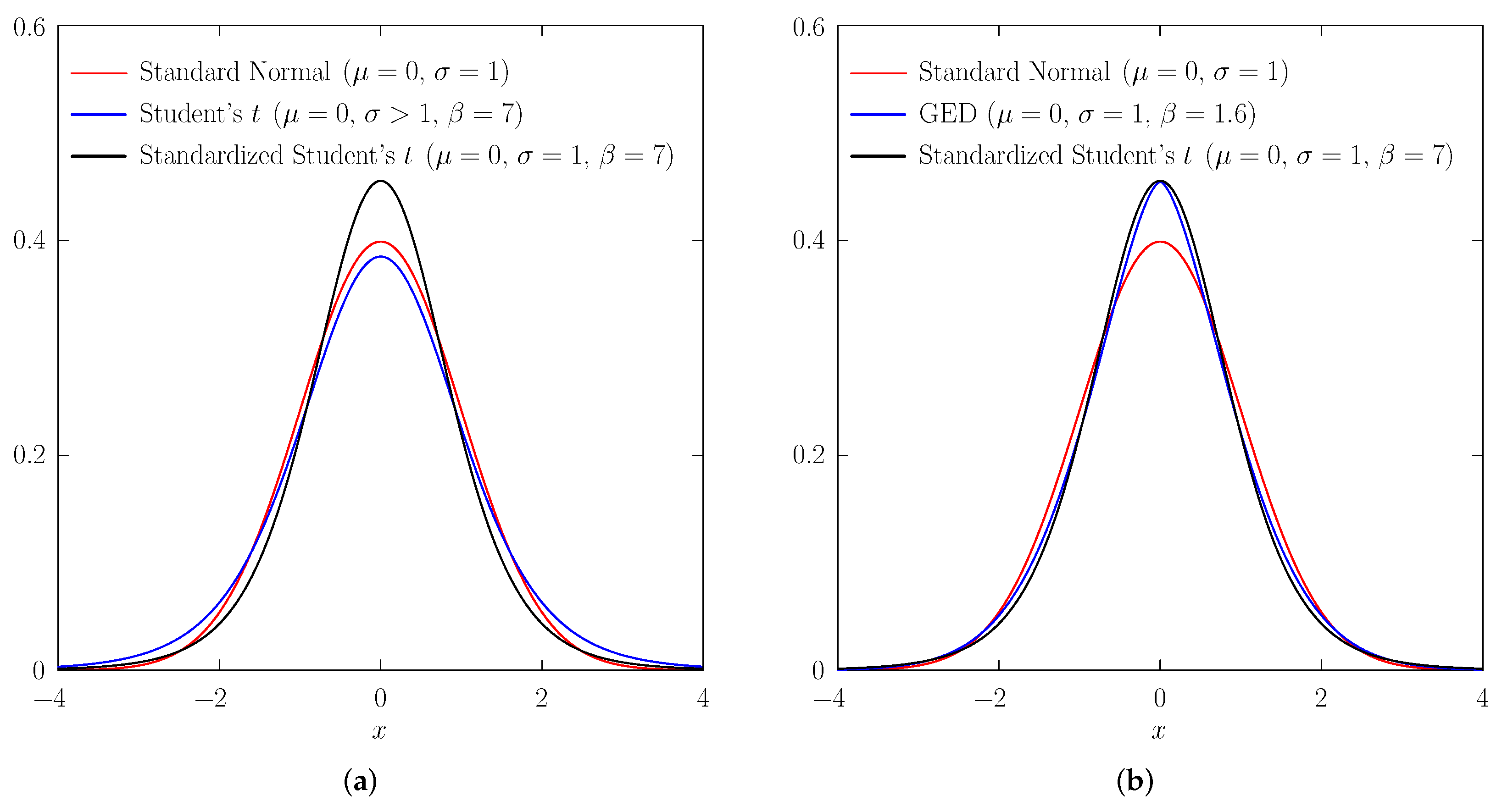
The next popular distribution is Student’s t, which is presented in Figure 1a. There are two kinds of Student’s t distribution. The first kind has a variance greater than one and is usually applied in regression analysis and finance. It has noticeable heavy tails and excess kurtosis, but its peak is lower than in normal distribution. If the distributional assumption is needed for standardized residuals with zero mean and unit variance, then one can apply the second kind of Student’s t distribution, which has unit variance, less noticeable heavy tails, excess kurtosis, and a peak higher than in normal distribution. Student’s t distribution is applied in [17] for modeling log of daily average prices of the European electricity markets. The authors of [35] considered normal and Student’s t distributions for volatility modeling. Student’s t distribution is similarly applied in [5] for modeling crude oil price volatility and [11] for modeling crude oil and natural gas spot and futures returns.

Generalized error distribution (GED), which is presented in Figure 1b, can also allow for heavy tails, excess kurtosis, and a higher peak than in normal distribution. GED is also called exponential power distribution [38]. This distribution has not been used as often as normal or Student’s t distribution, although tails under GED could be heavier than under Student’s t distribution with unit variance. The author of [25] states that because of heavy tails, results based on GED are more encouraging. Another difference is related to the shape of the peak. In GED the peak is acute and in Student’s t distribution the peak is smooth. The authors of [39] showed that assuming GED may allow achieving a higher value of the maximum likelihood function. In the paper, the authors concluded that models assuming a leptokurtic distribution (i.e., GED with a shape parameter below two reflecting a higher peak and heavy tails) seem most appropriate. Ref. [21] applies this distribution in estimating volatility of daily average prices from the England and Wales electricity market. The authors of [3] model crude oil prices using normal distribution, Student’s t distribution, and GED to evaluate out-of-sample forecasting performance. The research finds that Student’s t distribution is superior because of the high kurtosis in the oil return volatility.

Normal, Student’s t, and GED share one common drawback: they all impose symmetry. This drawback is resolved by introducing the asymmetry parameter $\chi$ (also known as a skewness parameter). The authors of [40] introduced skew generalized error distribution (SGED), the author of [41] introduced skew Student’s t distribution with unit variance (SST), the author of [42] introduced generalized hyperbolic distribution (GHYP), and the author of [43] introduced Johnson’s $S_U$ distribution (JSU). These flexible distributions include normal distribution and several other distributions as a special or limiting case. They allow taking into account asymmetry, heavy tails, and excess kurtosis usually observed in data or model residuals.

SGED, SST, GHYP, and JSU distributions have been applied in various areas. The authors of [44] found that forecasts of returns of the US Real Estate Investment Trust based on SGED are more accurate than those based on normal and Student’s t distributions. The author of [45] compares the value at risk model under normal distribution, GED, and SGED and found that SGED provides the best forecast performance. SGED was also used in [46] for modeling European call option prices, in [22,47] for modeling electricity prices, and in [48] for modeling daily returns of carbon prices.

The study [41] is the seminal study applying SST for volatility modeling. The author explains the ignorance of higher-order moments of the conditional distribution in other studies by the possible significant excitement that the conditional mean and variance already generate. The lack of excitement should not imply that higher-order moments can be completely ignored because they may be necessary for efficient estimation of parameters and accurate prediction. The authors of [49] show that even if assuming SST in volatility modeling is theoretically more appealing, SST does not necessarily deliver improved prediction when compared with normal distribution. We explain the discrepancy of conclusions in [41,49] by a possibility that the time series data studied in [49] could have been modeled by applying other flexible distributions like SGED or GHYP.

GHYP distribution is applied in [42] for modeling grain size distributions of wind blown sands and in [50] for returns of daily prices of shares. According to [51], hyperbolic distributions are much better for modeling skewness and kurtosis observed in data. Normal inverse Gaussian distribution representing a special case of GHYP is applied in [52] for modeling log returns of financial contracts traded in the Nordic electricity market. Normal, Student’s t, and GHYP distributions for modeling and forecasting volatility of petroleum futures were considered in [6].

JSU distribution has the advantage that it can be used when the empirical distribution has long tails [43]. This distribution is applied in [53] for American option pricing. The authors of [18] considered several distributions for modeling and forecasting intra-day price spreads on the German electricity market. Based on the Akaike information criterion (AIC), the research concludes that JSU is not the distribution of best fit. This result is questionable because the AIC is used for model selection and not for the distributional goodness of fit test.

3. Methodology

First, we describe the volatility model introduced in [23] and then present suggested modifications. Let us consider time series $y_t$ representing in our research the log of the wholesale electricity price (i.e., system marginal price (SMP)) of the peak-demand period during day t, that is, $lsm{p}_t$. If ${\psi }_{t-1}$ is the information set at time $t-1$ and $x_t$ is an exogenous variable, then [23] defines $y_t=E\left(x_t|{\psi }_{t-1}\right)+{\epsilon }_t$, where E denotes the conditional expectation operator, ${\psi }_{t-1}$ is used in the expectation operator to denote expected value conditional on past information (e.g., conditional on past prices), and ${\epsilon }_t$ is the disturbance term such that ${\epsilon }_t|{\psi }_{t-1}$ follows $\mathcal{N}(0,h_t)$. Here, $h_t$ denotes volatility defined as a linear function of past squared residuals in the following way: $h_t={\alpha }_0+{\alpha }_1{\epsilon }_{t-1}^2+\cdots +{\alpha }_p{\epsilon }_{t-p}^2$. The latter is called an autoregressive conditional heteroscedasticity process of order p denoted as ARCH(p).

We consider two modifications to the original volatility model introduced in [23]. First, we suggest that both $y_t$ and $h_t$ may depend on exogenous variables. This modification is common in the literature. Second, we suggest replacing normal distribution with SGED, SST, GHYP, or JSU. They nest normal distribution and several other distributions as a special or limiting case. The second modification is relatively new and reflects the fact that the model residuals usually tend to have an empirical distribution different from normal distribution because of asymmetry, heavy tails, or excess kurtosis. The correctness of the assumed theoretical distribution for model residuals is crucial for the validity of the maximum likelihood method.

Therefore, we consider the following autoregressive and autoregressive conditional heteroscedasticity (AR–ARCH) model:

$$\mathrm{Mean} \mathrm{equation}:\hspace{1em}lsm{p}_t=a_0+{\displaystyle \sum }_{i=1}^P{a}_{i}lsmp{p}_{t-i}+w_t^{\prime }·b+{\epsilon }_t$$

(1)

$$\mathrm{Volatility} \mathrm{equation}:\hspace{1em}{h}_t={\alpha }_0+{\displaystyle \sum }_{i=1}^p{\alpha }_i{\epsilon }_{t-i}^2+{\gamma }_1·{\epsilon }_{t-1}^2·I_{t-1}+z_t^{\prime }·\delta$$

(2)

$$\mathrm{Distributional} \mathrm{assumption}:\hspace{1em}{v}_t=\frac{{\epsilon }_t}{\sqrt{h_t}} \mathrm{is} \mathsf{i}.\mathsf{i}.\mathsf{d}. \mathrm{SGED}, \mathrm{SST}, \mathrm{GHYP}, \mathrm{or} \mathrm{JSU}.$$

(3)

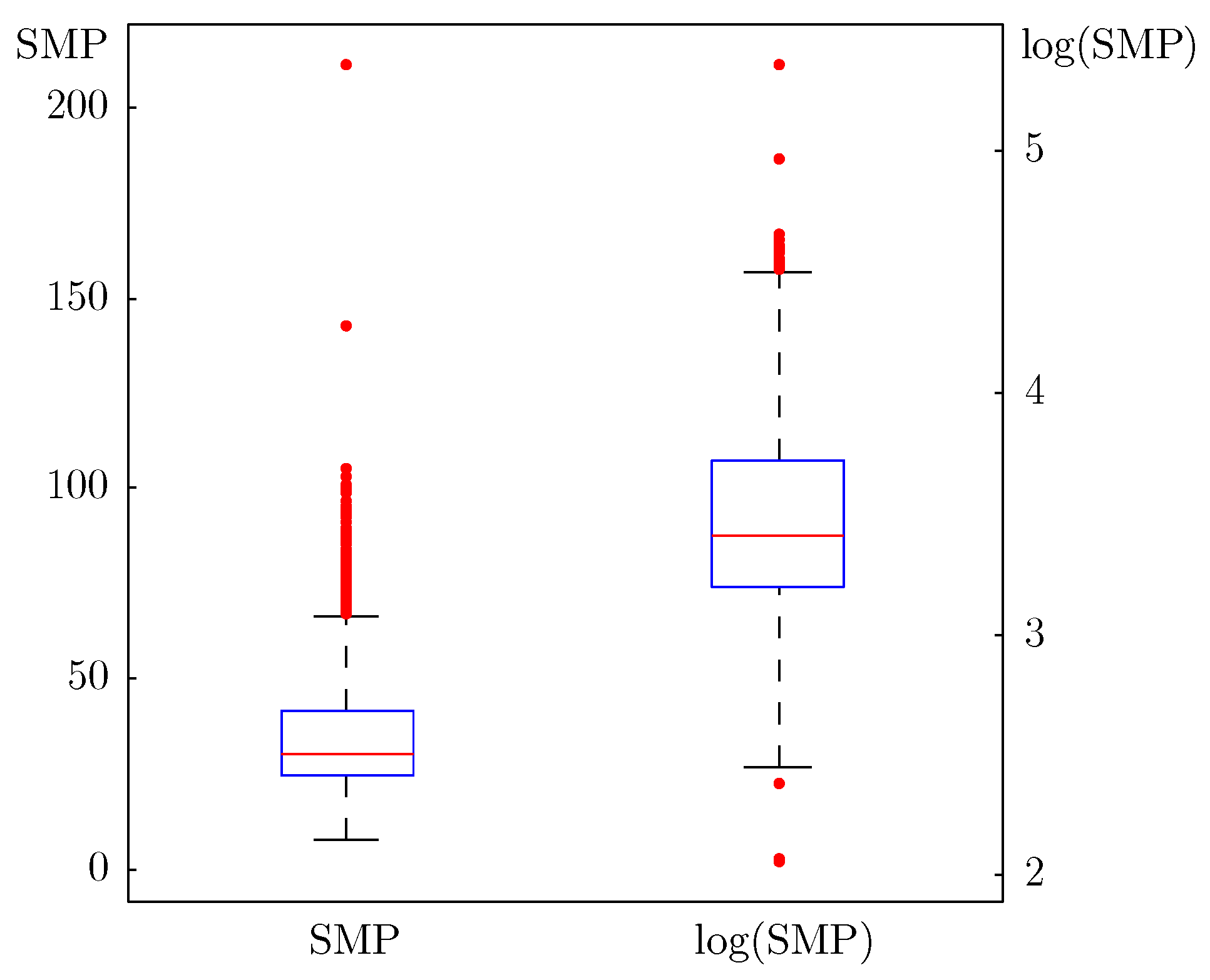
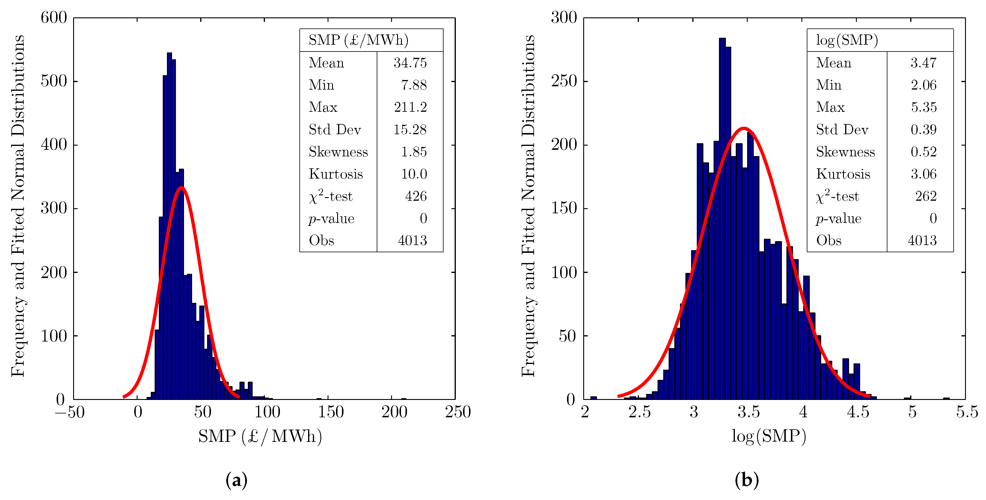
The first equation is called the mean equation and is analyzed using an autoregressive process with lag order P, that is, AR(P). In this equation, the dependent variable $lsm{p}_t$ represents the log of the system marginal price (SMP) of the peak-demand period during day t. The motivation of a logarithmic transformation is related to the fact that the influence of outliers is mitigated (as described in Figure 2) and that log prices tend to have a distribution closer to normal distribution (as described in Figure 3).

A logarithmic transformation is consistent with the methodology in [34], which analyzes total costs of distribution system operators depending on the number of subscribers, number of transformer substations, kilometers of high voltage grid, and the number of registered battery electric vehicles. As a case study, the authors analyze Norway, which has the highest share of electric vehicles. Because raw data are skewed to the right, ref. [34] applies log transformation in order to obtain data that have an empirical distribution closer to the normal distribution.

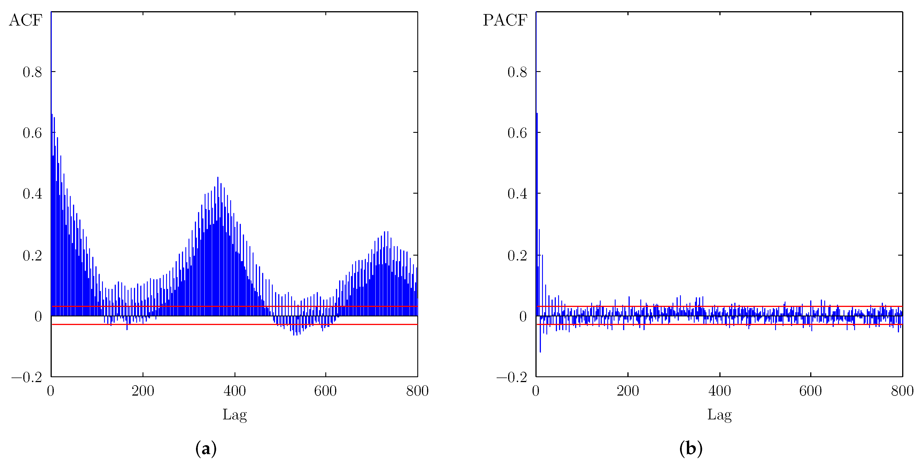
The dependent variable $lsm{p}_t$ is stationary, which allows applying the time and frequency domain analyses. The time domain analysis allows identifying statistically significant lags for the AR process. This analysis is performed using a correlogram that is presented in Figure 4. Statistically significant lags are needed for modeling the partial adjustment effects and periodicity pattern in electricity prices.

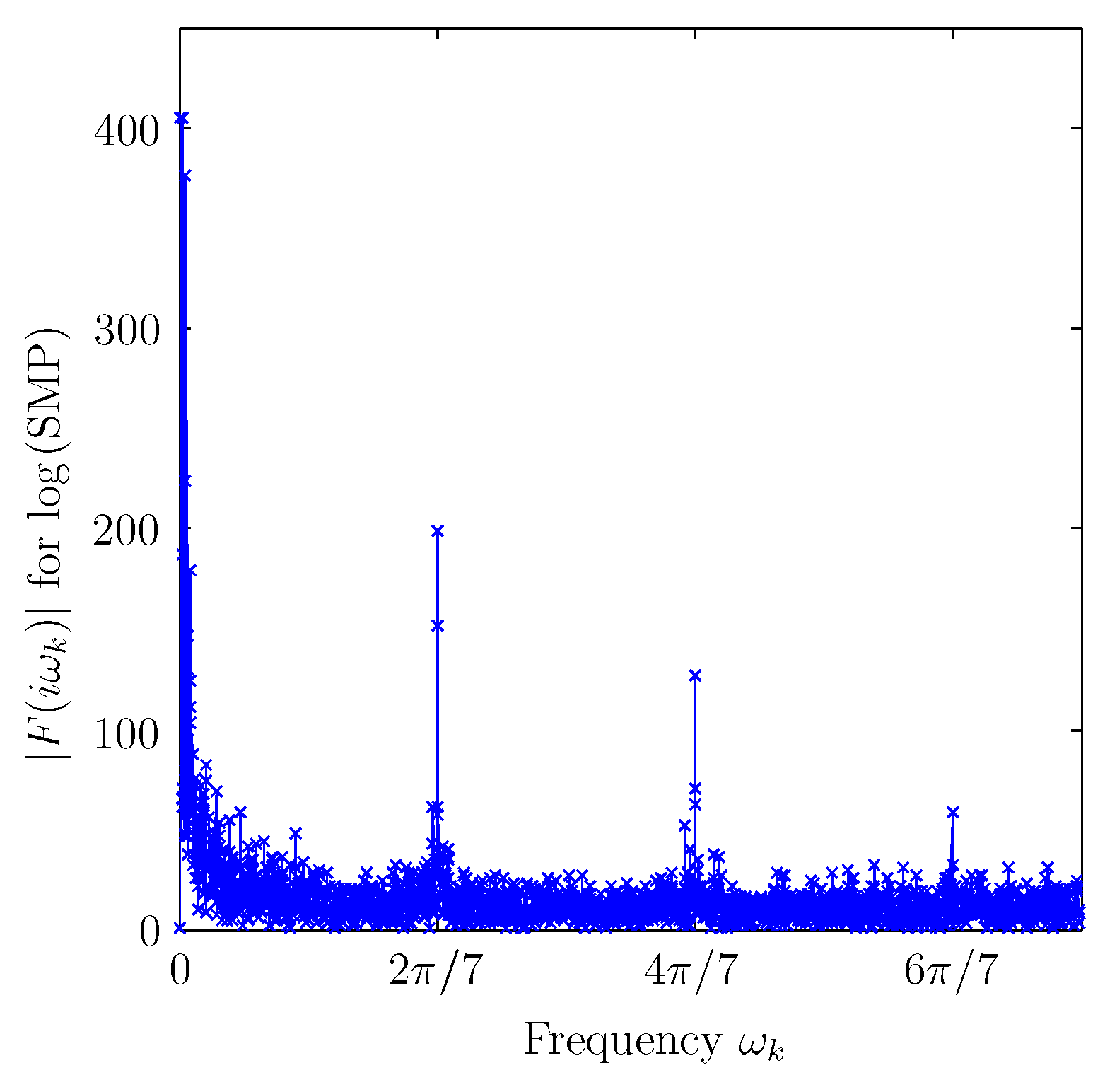
The frequency domain analysis presented in Figure 5 allows identifying frequencies in periodic functions. The inclusion of periodic functions as explanatory variables rules out the necessity to use some of the lags suggested by Figure 4 and the necessity to use the day of the week dummy variables for modeling weekly periodicity.

We use dummy variables for denoting regime periods in order to analyze the impact of regulatory reforms. The next explanatory variable included in vector $w_t$ in the mean Equation (1) is forecast demand for the peak-demand period of day t. Based on market rules in the England and Wales wholesale electricity market, forecast demand has been considered exogenous in determining the SMP. We do not include fuel prices because they are available only as quarterly average prices. We do not consider renewable energy sources either because they were not widely used during the analyzed period [54]. Finally, ${\epsilon }_t$ is the disturbance term such that $E\left({\epsilon }_t|{\psi }_{t-1}\right)=0$.

The volatility Equation (2) based on an ARCH(p) process is used for modeling heteroscedasticity in the disturbance term. This equation is augmented by a vector of explanatory variables $z_t$ including periodic functions and regime dummy variables. Following [26], we include the term ${\epsilon }_{t-1}^2·I_{t-1}$, where $I_{t-1}$ is an indicator function equal to 1 if ${\epsilon }_{t-1}<0$ and 0 otherwise. The latter allows taking into account the asymmetric effect of positive and negative shocks from the previous day on volatility.

The mean Equation (1) and volatility Equation (2) are jointly called an AR(P)–ARCH(p) model, which we extended by external regressors $w_t$ and $z_t$, respectively. To estimate these two equations jointly, we must make a distributional assumption for standardized residuals ${\nu }_t$ defined in Equation (3). We assume that ${\nu }_t$ are independent and identically distributed (i.i.d.) and follow SGED, SST, GHYP, or JSU. In the next section, we determine which flexible distribution is appropriate for our case study. The volatility model with all distributional assumptions satisfied allows analyzing the impact of regulatory reforms on price dynamics.

4. Estimation Results

We consider the SMP of the peak-demand period over trading days on the England and Wales electricity market. We concentrate on the analysis of prices from the peak-demand period over days because, as documented in the literature, firms usually tend to exercise market power namely during the peak-demand period, when even small changes in supply or demand may sometimes largely affect prices on the market. Various papers focused on the peak-demand period or specific weekday as well in order to analyze the market.

Table 1. Summary statistics of SMP of the peak-demand period during 1 April 1990–26 March 2001.

Price	Regime 1	Regime 2	Regime 3	Pre-Regime 4	Regime 4	Regime 5
	Apr 90–Mar 93	Apr 93–Mar 94	Apr 94–Mar 96	Apr 96–July 96	July 96–July 99	July 99–Mar 01
	Coal Contracts		Price-Cap Reg		Divestment 1	Divestment 2
Mean	25.66	32.90	37.22	35.25	41.99	35.91
Min	14.78	14.94	7.88	17.17	14.54	12.15
Max	62.97	55.95	211.24	76.74	105.09	77.89
St Dev	4.69	6.52	17.64	11.39	19.29	11.95
Coef of Var (%)	18.26	19.81	47.40	32.30	45.95	33.28
Obs	1096	365	731	91	1114	616

Sources: Office of Gas and Electricity Markets and [56]. Author’s calculations.

presents summary statistics of SMP across regulatory regime periods. A detailed description of introduced regulatory changes is provided in [55].

After coal contracts expired on 31 March 1993, price level and variance increased. During 1 April 1994–31 March 1996, price-cap regulation was introduced. It is interesting to observe a high level and a high variance of prices during the price-cap regulation period.

Later, divestment series were introduced in order to improve competition and reduce the influence of incumbent electricity producers. After the second series of divestments, the level and variance of prices declined. These observations motivate to model the dynamics of electricity prices.

The methodology for volatility modeling was described in Section 3. For estimating the parameters of the volatility model, we apply the maximum likelihood method, which besides data requires two more inputs. First, we must make a distributional assumption because, a priori, the correct distribution for standardized residuals defined in Equation (3) is unknown. We consider four flexible distributions (SGED, SST, GHYP, and JSU), which can take into account asymmetry or heavy tails instead of relying on their special cases that, for example, impose symmetry (like normal or Student’s t distributions).

Second, we must choose starting values for all parameters of the volatility model to avoid a failure of inverting the Hessian matrix or a failure of achieving convergence of the likelihood function. The starting values were chosen sequentially, where we began by estimating the simplest AR(1)–ARCH(1) model specification including regime dummy variables. Then, the AR(1) part was extended to include lags of the dependent variable and periodic functions that had a statistically significant correlation with the dependent variable $lsmp$. The estimation results for the final model specification satisfying the distributional assumption are presented in

Table 2. Estimation results based on the maximum likelihood method when assuming skew generalized error distribution, skew Student’s t distribution, generalized hyperbolic distribution, and Johnson’s $S_U$ distribution.

Assumed Distribution Intercepts and Variables		SGED $(\mathit{\mu },\mathit{\sigma },\mathit{\beta },\mathit{\chi })$		SST $(\mathit{\mu },\mathit{\sigma },\mathit{\beta },\mathit{\chi })$		GHYP $(\mathit{\mu },\mathit{\sigma },\mathit{\beta },\mathit{\chi },\mathit{\lambda })$		JSU $(\mathit{\mu },\mathit{\sigma },\mathit{\beta },\mathit{\chi })$
		Coef	Std Err	Coef	Std Err	Coef	Std Err	Coef	Std Err
Mean Equation	${\widehat{a}}_0$	−0.3728 ***	0.0147	−0.4892 ***	0.0872	−0.4976 ***	0.0936	−0.4792 ***	0.0803
	$lsm{p}_{t-1}$	0.3110 ***	0.0091	0.3066 ***	0.0069	0.3061 ***	0.0107	0.3069 ***	0.0019
	$lsm{p}_{t-2}$	0.1388 ***	0.0060	0.1422 ***	0.0195	0.1417 *	0.0730	0.1413 ***	0.0306
	$lsm{p}_{t-3}$	0.0362 ***	0.0022	0.0381	0.0258	0.0380	0.0278	0.0382 **	0.0186
	$lsm{p}_{t-4}$	0.0577 ***	0.0119	0.0569 ***	0.0214	0.0573 ***	0.0165	0.0572 ***	0.0165
	$lsm{p}_{t-6}$	0.1306 ***	0.0051	0.1304 ***	0.0192	0.1303 ***	0.0258	0.1303 ***	0.0270
	$lsm{p}_{t-7}$	0.1759 ***	0.0061	0.1705 ***	0.0308	0.1708 ***	0.0082	0.1713 ***	0.0192
	$lsm{p}_{t-9}$	−0.0486 ***	0.0096	−0.0468	0.0310	−0.0468 *	0.0282	−0.0472 **	0.0193
	$lsm{p}_{t-12}$	−0.0484 ***	0.0065	−0.0445 **	0.0217	−0.0441 **	0.0175	−0.0446 ***	0.0172
	$lsm{p}_{t-14}$	0.1320 ***	0.0052	0.1275 ***	0.0179	0.1276 ***	0.0204	0.1281 ***	0.0206
	$lsm{p}_{t-16}$	−0.0421 ***	0.0076	−0.0422 *	0.0248	−0.0421 **	0.0198	−0.0421 **	0.0165
	$lsm{p}_{t-21}$	0.0988 ***	0.0043	0.1020 ***	0.0168	0.1022 ***	0.0185	0.1017 ***	0.0186
	$lsm{p}_{t-22}$	−0.0534 ***	0.0063	−0.0546 ***	0.0191	−0.0550 ***	0.0162	−0.0551 ***	0.0163
	$lsm{p}_{t-51}$	−0.0449 ***	0.0090	−0.0435 ***	0.0151	−0.0438 ***	0.0131	−0.0437 ***	0.0127
	$lsm{p}_{t-56}$	0.0372 ***	0.0040	0.0386 **	0.0151	0.0390 ***	0.0129	0.0388 ***	0.0121
	$lsm{p}_{t-164}$	−0.0286 ***	0.0048	−0.0264 **	0.0123	−0.0265	0.0177	−0.0267 ***	0.0065
	$lsm{p}_{t-364}$	0.0669 ***	0.0107	0.0655 ***	0.0111	0.0655 ***	0.0112	0.0654 ***	0.0102
	$ldeman{d}_t$	0.0616 ***	0.0015	0.0723 ***	0.0028	0.0731 ***	0.0051	0.0714 ***	0.0006
	Regime 2	0.0206 ***	0.0055	0.0201 **	0.0082	0.0203	0.0144	0.0202 ***	0.0056
	Regime 3	0.0353 ***	0.0097	0.0344 ***	0.0114	0.0354 *	0.0196	0.0352 ***	0.0087
	Pre-Regime 4	0.0246	0.0325	0.0273	0.0334	0.0287	0.0377	0.0277	0.0321
	Regime 4	0.0315 ***	0.0087	0.0286 **	0.0127	0.0294	0.0237	0.0295 ***	0.0060
	Regime 5	−0.0037	0.0097	−0.0023	0.0121	−0.0019	0.0187	−0.0020	0.0084
	$sin(2\pi t/7)$	0.0080 **	0.0033	0.0079 **	0.0039	0.0079 *	0.0043	0.0079 **	0.0040
	$cos(2\pi t/7)$	−0.0136 ***	0.0021	−0.0141 ***	0.0040	−0.0138 ***	0.0040	−0.0139 ***	0.0040
	$sin(4\pi t/7)$	−0.0111 ***	0.0029	−0.0117 ***	0.0037	−0.0115 ***	0.0036	−0.0114 ***	0.0036
	$cos(4\pi t/7)$	−0.0117 ***	0.0033	−0.0115 ***	0.0035	−0.0114 ***	0.0036	−0.0115 ***	0.0036
	$cos(6\pi t/7)$	0.0105 ***	0.0033	0.0105 ***	0.0035	0.0106 ***	0.0034	0.0104 ***	0.0034
Volatility Equation	${\widehat{\alpha }}_0$	0.0037 ***	0.0005	0.0037 ***	0.0006	0.0037 ***	0.0005	0.0036 ***	0.0005
	${\epsilon }_{t-1}^2$	0.1571 ***	0.0367	0.1653 ***	0.0386	0.1674 ***	0.0395	0.1646 ***	0.0383
	${\epsilon }_{t-2}^2$	0.0810 ***	0.0205	0.0903 ***	0.0219	0.0900 ***	0.0216	0.0888 ***	0.0215
	${\epsilon }_{t-4}^2$	0.0314 **	0.0156	0.0229	0.0166	0.0218	0.0164	0.0242	0.0162
	${\epsilon }_{t-5}^2$	0.0412 **	0.0194	0.0378 *	0.0195	0.0388 *	0.0208	0.0385 **	0.0193
	${\epsilon }_{t-6}^2$	0.0761 ***	0.0244	0.0776 ***	0.0245	0.0785 ***	0.0246	0.0780 ***	0.0246
	${\epsilon }_{t-7}^2$	0.0903 ***	0.0247	0.1091 ***	0.0271	0.1101 ***	0.0280	0.1066 ***	0.0261
	${\epsilon }_{t-9}^2$	0.0961 ***	0.0224	0.0941 ***	0.0226	0.0922 ***	0.0225	0.0933 ***	0.0223
	${\epsilon }_{t-1}^2·I_{t-1}$	0.0802	0.0522	0.0882	0.0539	0.0829	0.0540	0.0845	0.0534
	Regime 2	0.0038 ***	0.0011	0.0041 ***	0.0012	0.0041 ***	0.0012	0.0040 ***	0.0012
	Regime 3	0.0287 ***	0.0038	0.0277 ***	0.0040	0.0283 ***	0.0040	0.0280 ***	0.0040
	Pre-Regime 4	0.0547 ***	0.0179	0.0559 ***	0.0183	0.0570 ***	0.0184	0.0559 ***	0.0182
	Regime 4	0.0336 ***	0.0042	0.0324 ***	0.0043	0.0326 ***	0.0044	0.0325 ***	0.0043
	Regime 5	0.0280 ***	0.0043	0.0275 ***	0.0045	0.0279 ***	0.0045	0.0275 ***	0.0044
	$sin(2\pi t/7)$	0.0031 ***	0.0006	0.0034 ***	0.0006	0.0033 ***	0.0007	0.0033 ***	0.0006
	$\widehat{\beta }$	1.4254 ***	0.0459	6.8967 ***	0.7803	0.0290 **	0.0130	1.9448 ***	0.1241
	$\widehat{\chi }$	1.0539 ***	0.0225	1.0431 ***	0.0253	0.9946 ***	0.0007	0.1625 **	0.0759
	$\widehat{\lambda }$					−3.4734 ***	0.3959

Notes: We take into account the asymmetries in the volatility process by introducing the term ${\epsilon }_{t-1}^2·I_{t-1}$. Even if this term’s p-value is slightly above 0.10 in the estimated model based on SGED, it was necessary to keep this term in order to satisfy the sign bias test. *, **, and *** stand for the 10%, 5%, and 1% significance levels, respectively.

.

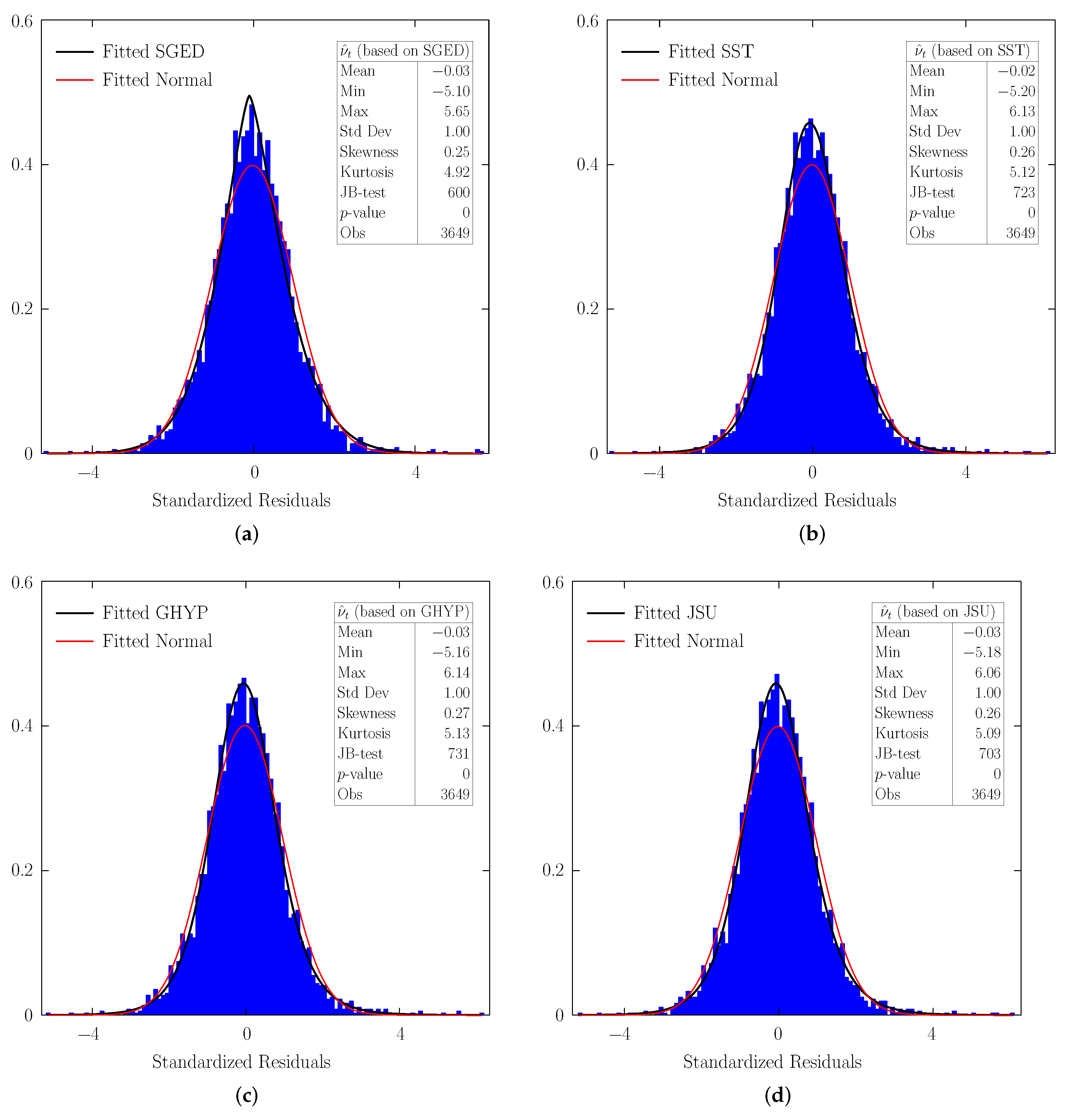
The distributional assumptions of SGED, SST, GHYP, and JSU for standardized residuals ${\widehat{\nu }}_t$ are not rejected by the goodness of fit test. Figure 6 depicts a good fit between the empirical distribution of standardized residuals and assumed theoretical distribution in all four volatility models. The Kullback–Leibler distance introduced in [57] can be used in evaluating the fit between the empirical and chosen theoretical distributions. In our research, this approach was inconclusive because only for certain choices of the number of values in the nearest neighbor search algorithm was the Kullback–Leibler distance between the empirical distribution of standardized residuals and fitted SGED smaller than under fitted SST, GHYP, and JSU distributions.

Residuals from any model must be random, more precisely, independent and identically distributed (i.i.d). This can be verified using the BDS-test further developed in [58]. We perform the BDS-test of i.i.d. for ${\widehat{\nu }}_t$ and ${\widehat{\nu }}_t^2$ from each of the volatility models based on SGED, SST, GHYP, and JSU distributions. When ${\widehat{\nu }}_t$ is i.i.d, then ${\widehat{\nu }}_t$ is not serially correlated. Similarly, when ${\widehat{\nu }}_t^2$ is i.i.d, then ${\widehat{\nu }}_t$ is not heteroscedastic. The results are presented in

Table 3. p-values of the BDS-test for ${\widehat{\nu }}_t$, ${\widehat{\nu }}_t^2$, ${\widehat{\nu }}_t^3$, and ${\widehat{\nu }}_t^4$.

		SGED				SST				GHYP				JSU
		${\widehat{\mathbf{\nu }}}_{\mathit{t}}$	${\widehat{\mathbf{\nu }}}_{\mathit{t}}^{\mathbf{2}}$	${\widehat{\mathbf{\nu }}}_{\mathit{t}}^{\mathbf{3}}$	${\widehat{\mathbf{\nu }}}_{\mathit{t}}^{\mathbf{4}}$	${\widehat{\mathbf{\nu }}}_{\mathit{t}}$	${\widehat{\mathbf{\nu }}}_{\mathit{t}}^{\mathbf{2}}$	${\widehat{\mathbf{\nu }}}_{\mathit{t}}^{\mathbf{3}}$	${\widehat{\mathbf{\nu }}}_{\mathit{t}}^{\mathbf{4}}$	${\widehat{\mathbf{\nu }}}_{\mathit{t}}$	${\widehat{\mathbf{\nu }}}_{\mathit{t}}^{\mathbf{2}}$	${\widehat{\mathbf{\nu }}}_{\mathit{t}}^{\mathbf{3}}$	${\widehat{\mathbf{\nu }}}_{\mathit{t}}^{\mathbf{4}}$	${\widehat{\mathbf{\nu }}}_{\mathit{t}}$	${\widehat{\mathbf{\nu }}}_{\mathit{t}}^{\mathbf{2}}$	${\widehat{\mathbf{\nu }}}_{\mathit{t}}^{\mathbf{3}}$	${\widehat{\mathbf{\nu }}}_{\mathit{t}}^{\mathbf{4}}$
Dimension	2	0.46	0.13	0.15	0.23	0.30	0.09	0.09	0.11	0.31	0.09	0.09	0.15	0.32	0.10	0.10	0.15
	3	0.30	0.15	0.12	0.17	0.13	0.08	0.06	0.07	0.15	0.08	0.06	0.11	0.15	0.09	0.06	0.10
	4	0.12	0.18	0.12	0.20	0.04	0.08	0.06	0.10	0.04	0.09	0.06	0.13	0.05	0.10	0.07	0.13
	5	0.07	0.32	0.17	0.32	0.03	0.18	0.10	0.19	0.03	0.21	0.10	0.24	0.03	0.22	0.11	0.23
	6	0.10	0.68	0.40	0.71	0.05	0.46	0.30	0.52	0.06	0.51	0.30	0.57	0.05	0.52	0.32	0.55

.

The p-value of the BDS-test for standardized residuals ${\widehat{\nu }}_t$ is frequently below 0.10 when assuming SST, GHYP, and JSU distributions. The result suggests that ${\widehat{\nu }}_t$ is not i.i.d. in the volatility models based on the SST, GHYP, and JSU distributions. We also find a similar result for ${\widehat{\nu }}_t^2$.

Skewness and kurtosis represent the third and fourth standardized moments, respectively. That is why we additionally test if ${\widehat{\nu }}_t^3$ and ${\widehat{\nu }}_t^4$ are i.i.d., which is partly consistent with the suggestion in [41]. The BDS-test suggests that ${\widehat{\nu }}_t^3$ are not i.i.d. in the volatility models assuming SST, GHYP, and JSU distributions. This could be related to the violation of the i.i.d. assumption for standardized residuals ${\widehat{\nu }}_t$ in those volatility models.

Last, we perform the sign bias test, where the null hypothesis states that the volatility model is correctly specified. The results are presented in

Table 4. Test values of the sign bias test for standardized residuals ${\widehat{\nu }}_t$.

	Assumed Theoretical Distribution
	SGED	SST	GHYP	JSU
Sign Bias	0.45	0.12	0.13	0.14
Negative Sign Bias	1.28	1.35	1.33	1.33
Positive Sign Bias	1.55	1.91 *	1.90 *	1.88 *
Joint Effect	4.68	5.75	5.70	5.62

Notes: * stands for p-values between 0.05 and 0.10. The positive sign bias test rejects the null hypothesis stating that the volatility model is correctly specified when SST, GHYP, and JSU distributions are assumed.

.

The null hypothesis is rejected when assuming SST, GHYP, and JSU distributions because the p-value for the positive sign bias test is less than 0.10. Hence, based on the BDS-test and sign bias test, we conclude that assuming SGED for volatility modeling is appropriate in our case study.

5. Discussion

For volatility modeling, we verified the distributional assumption, i.i.d. assumption, and correctness of the specified volatility model. The distributional assumption states that model residuals follow a particular theoretical distribution. The empirical and assumed theoretical distributions can be analyzed using distribution plots or, more formally, using the goodness of fit test. The goodness of fit test suggested that SGED, SST, GHYP, and JSU distributions provided a good fit for the empirical distribution of standardized residuals.

Not always is the distributional assumption satisfied. The author of [59] addressed the model misspecification problem related to the wrong distributional assumption and proposed a quasi maximum likelihood method for robust statistical inference. This method is applied in [60] for modeling the dynamics of electricity prices from various countries. The research assumed a normal distribution, even if prices are asymmetric and have platykurtic and leptokurtic distributions. We believe that estimation results may be biased due to the wrong distributional assumption. In some cases, the distributional tests were applied incorrectly. For example, the authors of [18] relied on the AIC for choosing the appropriate distributional assumption.

We suggest assuming flexible distributions when the empirical distribution of data or model residuals has the features of asymmetry, heavy tails, or excess kurtosis that may lead to a parsimonious model. Using more complex volatility models with normal or Student’s t distribution assumed may not be fully correct (e.g., [7,61]).

After the distributional assumption, we must verify if model residuals are random, that is, independent and identically distributed (i.i.d.), which suggests that residuals do not have serial correlation and heteroscedasticity problems. However, some papers do not discuss whether model residuals are serially correlated or heteroscedastic. For example, residuals from most of GARCH-type estimated models presented in Tables 3–6 in [5] had a serial correlation and heteroscedasticity problems. In such cases, the estimates are biased and we cannot apply hypothesis testing.

Based on the BDS-test and sign bias test, we find that SGED is the appropriate distribution for volatility modeling in our case study. Based on the correctly estimated volatility model, we can analyze the effect of demand and reforms. We estimate that a 1% increase in forecast demand is expected to increase the electricity price by 0.06%.

The effect of reforms is analyzed using regime dummy variables. High coefficient estimates in front of the Regime 2 dummy variable in the mean and volatility equations presented in Table 2 suggest that after the coal contracts expired in March 1993, price level and volatility increased. Later, price level and volatility increased further during price-cap regulation (i.e., during Regime 3). Higher price volatility during price-cap regulation may stem from different bidding strategies during the peak-demand period over weekdays and weekends. A similar finding was already described in [21] but based on daily average prices. Focusing on prices of the peak-demand period over days is sometimes more important than analyzing average prices because firms may be more inclined to exercise market power namely during the peak-demand period. Another approach to account for this possible strategy is to analyze demand weighted average prices (e.g., in [62]). However, this approach may not always be feasible due to limitations or incompleteness of data on demand for electricity.

As presented in Table 2, coefficient estimates in front of the Regime 5 dummy variable in the mean and volatility equations are lower than coefficient estimates in front of the Regime 3 and Regime 4 dummy variables. The result suggests that price level and volatility declined after the second series of divestments. Hence, the second series of divestments was more successful at lowering price level and volatility than the price-cap regulation and the first series of divestments.

6. Conclusions and Policy Implications

Modeling energy prices has been of interest to investors, producers, and market regulators. We suggest using flexible distributions that account for such features as asymmetry, heavy tails, or excess kurtosis. A correct distributional assumption is necessary when using the maximum likelihood method. The advantage of using flexible distributions, for example, even for symmetric data or errors, is that the estimate of the skewness parameter of the flexible distribution will confirm symmetry without loss of generality. The application of flexible distributions may lead to a simpler and parsimonious model allowing for more precise forecasts, economic evaluation, planning, and policy recommendations. The authors of [32] highlighted the importance of correct modeling of price volatility for building accurate pricing models, for forecasting future price volatility, and for enriching our understanding of the broader financial markets, the energy industry, and the overall economy. The presented volatility model can be adapted or extended for analyzing other energy markets. For this purpose, one may include new exogenous variables accounting for fuel prices, renewable energy sources, various events like the COVID-19 pandemic, etc.

We find that after the second series of divestments, price level and volatility reduced compared to the price-cap regulation period and the first series of divestments. Therefore, we conclude that a sufficient horizontal restructuring through divestment series may indeed be successful at lowering prices and volatility on the market. On the one hand, lower prices for goods and services of general interest are essential for consumers. On the other hand, lower price volatility may be preferred by producers willing to minimize the uncertainty about their revenues or profits, which could motivate producers to increase investments.

Generally, a horizontal restructuring through divestment series may allow reducing the ability of dominant producers to affect prices. In particular, dominant producers may decide to withhold part of their production capacity in order to increase prices and subsequently achieve higher profits [54]. For example, the European Commission investigated the E.ON AG producer for abusing its dominant position to withhold available production facilities on the German electricity market in order to raise prices [63]. Later, it was agreed that the producer would divest about 20% of its generation capacity in Germany. However, not in all countries is it possible to introduce divestment series. For example, Australia is planning to introduce amendments to the Competition and Consumer Act 2010 [64]. The amendments will allow the introduction of divestments in order to force electricity wholesalers to sell a business or asset if they engage in certain pricing breaches.

A horizontal restructuring through divestment series may be preferred to price-cap regulation because the latter is associated with monitoring costs. This reasoning probably explains why the European Commission decided to choose divestments and Australia decided to introduce amendments to the Act. Our research confirms that divestment series may indeed be successful at lowering prices without any need for further monitoring that the price-cap regulation would have required.

References

- Hadsell, L.; Marathe, A.; Shawky, H.A. Estimating the volatility of wholesale electricity spot prices in the US. Energy J. 2004, 25, 23–40. [Google Scholar] [CrossRef] [Green Version]
- Bessembinder, H.; Lemmon, M.L. Equilibrium pricing and optimal hedging in electricity forward markets. J. Financ. 2002, 57, 1347–1382. [Google Scholar] [CrossRef]
- Herrera, A.M.; Hu, L.; Pastor, D. Food price volatility and macroeconomic factors: Evidence from GARCH and GARCH-X estimates. Int. J. Forecast. 2018, 34, 622–635. [Google Scholar] [CrossRef]
- Ziel, F.; Weron, R. Day-ahead electricity price forecasting with high-dimensional structures: Univariate vs. multivariate modeling frameworks. Energy Econ. 2018, 70, 396–420. [Google Scholar] [CrossRef] [Green Version]
- Zhang, Y.J.; Yao, T.; Ripple, R. Volatility forecasting of crude oil market: Can the regime switching GARCH model beat the single-regime GARCH models? Int. Rev. Econ. Financ. 2019, 59, 302–317. [Google Scholar] [CrossRef]
- Hasanov, A.S.; Shaiban, M.S.; Al-Freedi, A. Forecasting volatility in the petroleum futures markets: A re-examination and extension. Energy Econ. 2020, 86, 104626. [Google Scholar] [CrossRef]
- Nonejad, N. Crude oil price volatility and equity return predictability: A comparative out-of-sample study. Int. Rev. Financ. Anal. 2020, 71, 101521. [Google Scholar] [CrossRef]
- Dutta, A.; Bouri, E.; Roubaud, D. Modelling the volatility of crude oil returns: Jumps and volatility forecasts. Int. J. Financ. Econ. 2021, 26, 889–897. [Google Scholar] [CrossRef]
- Kocaarslan, B.; Soytas, U. Reserve currency and the volatility of clean energy stocks: The role of uncertainty. Energy Econ. 2021, 104, 105645. [Google Scholar] [CrossRef]
- Luo, J.; Demirer, R.; Gupta, R.; Ji, Q. Forecasting oil and gold volatilities with sentiment indicators under structural breaks. Energy Econ. 2022, 105, 105751. [Google Scholar] [CrossRef]
- Xu, Y.; Lien, D. Forecasting volatilities of oil and gas assets: A comparison of GAS, GARCH, and EGARCH models. J. Forecast. 2022, 41, 259–278. [Google Scholar] [CrossRef]
- Bowden, N.; Payne, J.E. Short term forecasting of electricity prices for MISO hubs: Evidence from ARIMA-EGARCH models. Energy Econ. 2008, 30, 3186–3197. [Google Scholar] [CrossRef]
- Escribano, A.; Peña, J.I.; Villaplana, P. Modelling electricity prices: International evidence. Oxf. Bull. Econ. Stat. 2011, 73, 622–650. [Google Scholar] [CrossRef] [Green Version]
- Geman, H.; Roncoroni, A. Understanding the fine structure of electricity prices. J. Bus. 2006, 79, 1225–1261. [Google Scholar] [CrossRef] [Green Version]
- Zhou, F.; Huang, Z.; Zhang, C. Carbon price forecasting based on CEEMDAN and LSTM. Appl. Energy 2022, 311, 118601. [Google Scholar] [CrossRef]
- Evans, J.E.; Green, R.J. Why Did British Electricity Prices Fall after 1998? MIT Center for Energy and Environmental Policy Research Working Paper Series No. 03-007; MIT Center: Cambridge, MA, USA, 2003. [Google Scholar]
- Koopman, S.J.; Ooms, M.; Carnero, M.A. Periodic seasonal Reg-ARFIMA-GARCH models for daily electricity spot prices. J. Am. Stat. Assoc. 2007, 102, 16–27. [Google Scholar] [CrossRef] [Green Version]
- Abramova, E.; Bunn, D. Forecasting the intra-day spread densities of electricity prices. Energies 2020, 13, 687. [Google Scholar] [CrossRef] [Green Version]
- Joskow, P.L. Foreword: US vs. EU Electricity Reforms Achievement. In Electricity Reform in Europe; Glachant, J.M., Lévêque, F., Eds.; Edward Elgar Publishing Limited: Cheltenham, UK, 2009. [Google Scholar]
- Robinson, T.; Baniak, A. The volatility of prices in the English and Welsh electricity pool. Appl. Econ. 2002, 34, 1487–1495. [Google Scholar] [CrossRef]
- Tashpulatov, S.N. Estimating the volatility of electricity prices: The case of the England and Wales wholesale electricity market. Energy Policy 2013, 60, 81–90. [Google Scholar] [CrossRef] [Green Version]
- Tashpulatov, S.N. The impact of behavioral and structural remedies on electricity prices: The case of the England and Wales electricity market. Energies 2018, 11, 3420. [Google Scholar] [CrossRef] [Green Version]
- Engle, R.F. Autoregressive conditional heteroscedasticity with estimates of the variance of United Kingdom inflation. Econometrica 1982, 50, 987–1007. [Google Scholar] [CrossRef]
- Bollerslev, T. Generalized autoregressive conditional heteroscedasticity. J. Econom. 1986, 31, 307–327. [Google Scholar] [CrossRef] [Green Version]
- Nelson, D.B. Conditional heteroskedasticity in asset returns: A new approach. Econometrica 1991, 59, 347–370. [Google Scholar] [CrossRef]
- Glosten, L.R.; Jagannathan, R.; Runkle, D.E. On the relation between the expected value and the volatility of the nominal excess returns on stocks. J. Financ. 1993, 48, 1779–1801. [Google Scholar] [CrossRef]
- Hansen, P.R.; Lunde, A. A forecast comparison of volatility models: Does anything beat a GARCH(1,1)? J. Appl. Econom. 2005, 20, 873–889. [Google Scholar] [CrossRef] [Green Version]
- Charles, A.; Darné, O. Forecasting crude-oil market volatility: Further evidence with jumps. Energy Econ. 2017, 67, 508–519. [Google Scholar] [CrossRef]
- Ergen, I.; Rizvanoghlu, I. Asymmetric impacts of fundamentals on the natural gas futures volatility: An augmented GARCH approach. Energy Econ. 2016, 56, 64–74. [Google Scholar] [CrossRef]
- Klein, T.; Walther, T. Oil price volatility forecast with mixture memory GARCH. Energy Econ. 2016, 58, 46–58. [Google Scholar] [CrossRef] [Green Version]
- Jarque, C.M.; Bera, A.K. A test for normality of observations and regression residuals. Int. Stat. Rev. 1987, 55, 163–172. [Google Scholar] [CrossRef]
- Ewing, B.; Malik, F. Modelling asymmetric volatility in oil prices under structural breaks. Energy Econ. 2017, 63, 227–233. [Google Scholar] [CrossRef]
- Shalini, V.; Prasanna, K. Impact of the financial crisis on Indian commodity markets: Structural breaks and volatility dynamics. Energy Econ. 2016, 53, 40–57. [Google Scholar] [CrossRef]
- Wangsness, P.B.; Halse, A.H. The impact of electric vehicle density on local grid costs: Empirical evidence from Norway. Energy J. 2021, 42, 149–167. [Google Scholar] [CrossRef]
- Koopman, S.J.; Lukas, A.; Scharth, M. Predicting time-varying parameters with parameter-driven and observation-driven models. Rev. Econ. Stat. 2016, 98, 97–110. [Google Scholar] [CrossRef] [Green Version]
- Gosset, W.S. The probable error of a mean. Biometrika 1908, 6, 1–24. [Google Scholar]
- Subbotin, M.T.H. On the law of frequency of error. Mat. Sb. 1923, 31, 296–301. [Google Scholar]
- Box, G.E.P.; Tiao, G.C. Bayesian Inference in Statistical Analysis; Addison-Wesley Publishing Co.: Reading, MA, USA, 1973. [Google Scholar]
- Bosco, B.P.; Parisio, L.P.; Pelagatti, M.M. Deregulated wholesale electricity prices in Italy: An empirical analysis. Int. Adv. Econ. Res. 2007, 13, 415–432. [Google Scholar] [CrossRef]
- Fernández, C.; Steel, M. On Bayesian modeling of fat tails and skewness. J. Am. Stat. Assoc. 1998, 93, 359–371. [Google Scholar]
- Hansen, B.E. Autoregressive conditional density estimation. Int. Econ. Rev. 1994, 35, 705–730. [Google Scholar] [CrossRef]
- Barndorff-Nielsen, O.E. Exponentially decreasing distributions for the logarithm of particle size. Proc. R. Soc. Lond. A Math. Phys. Eng. Sci. 1977, 353, 401–419. [Google Scholar]
- Johnson, N.L. Systems of frequency curves derived from the first law of Laplace. Trab. Estad. 1954, 5, 283–291. [Google Scholar] [CrossRef]
- Lee, Y.H.; Pai, T.Y. REIT volatility prediction for skew-GED distribution of the GARCH model. Expert Syst. Appl. 2010, 37, 4737–4741. [Google Scholar] [CrossRef]
- Su, J.B. How to mitigate the impact of inappropriate distributional settings when the parametric value-at-risk approach is used. Quant. Financ. 2014, 14, 305–325. [Google Scholar] [CrossRef]
- Theodossiou, P. Skewed generalized error distribution of financial assets and option pricing. Multinatl. Financ. J. 2015, 19, 223–266. [Google Scholar] [CrossRef] [Green Version]
- Ioannidis, F.; Kosmidou, K.; Savva, C.; Theodossiou, P. Electricity pricing using a periodic GARCH model with conditional skewness and kurtosis components. Energy Econ. 2021, 95, 105110. [Google Scholar] [CrossRef]
- Fu, Y.; Zheng, Z. Volatility modeling and the asymmetric effect for China’s carbon trading pilot market. Phys. A Stat. Mech. Its Appl. 2020, 542, 123401. [Google Scholar] [CrossRef]
- Frömmel, M.; Han, X.; Kratochvil, S. Modeling the daily electricity price volatility with realized measures. Energy Econ. 2014, 44, 492–502. [Google Scholar] [CrossRef]
- Eberlein, E.; Keller, U. Hyperbolic distributions in finance. Bernoulli 1995, 1, 281–299. [Google Scholar] [CrossRef]
- Küchler, U.; Neumann, K.; Sørensen, M.; Streller, A. Stock returns and hyperbolic distributions. Math. Comput. Model. 1999, 29, 1–15. [Google Scholar] [CrossRef]
- Frestad, D.; Benth, F.E.; Koekebakker, S. Modeling term structure dynamics in the Nordic electricity swap market. Energy J. 2010, 31, 53–86. [Google Scholar] [CrossRef] [Green Version]
- Simonato, J.G. American option pricing under GARCH with non-normal innovations. Optim. Eng. 2019, 20, 853–880. [Google Scholar] [CrossRef]
- Lízal, L.M.; Tashpulatov, S.N. Do producers apply a capacity cutting strategy to increase prices? The case of the England and Wales electricity market. Energy Econ. 2014, 43, 114–124. [Google Scholar] [CrossRef]
- Tashpulatov, S.N. Analysis of electricity industry liberalization in Great Britain: How did the bidding behavior of electricity producers change? Util. Policy 2015, 36, 24–34. [Google Scholar] [CrossRef] [Green Version]
- National Grid Company. Seven Year Statement; National Grid Company: Coventry, UK, 1994–2001. [Google Scholar]
- Kullback, S.; Leibler, R.A. On information and sufficiency. Ann. Math. Stat. 1951, 22, 16–27. [Google Scholar] [CrossRef]
- Brock, W.A.; Dechert, W.D.; Scheinkman, J.A.; LeBaron, B. A test for independence based on the correlation dimension. Econom. Rev. 1996, 15, 197–235. [Google Scholar] [CrossRef]
- White, H. Maximum likelihood estimation of misspecified models. Econometrica 1982, 50, 1–25. [Google Scholar] [CrossRef]
- Erdogdu, E. Asymmetric volatility in European day-ahead power markets: A comparative microeconomic analysis. Energy Econ. 2016, 56, 398–409. [Google Scholar] [CrossRef] [Green Version]
- Lin, Y.; Xiao, Y.; Li, F. Forecasting crude oil price volatility via a HM-EGARCH model. Energy Econ. 2020, 87, 104693. [Google Scholar] [CrossRef]
- Tashpulatov, S.N. The impact of regulatory reforms on demand weighted average prices. Mathematics 2021, 9, 1112. [Google Scholar] [CrossRef]
- European Commission. Summary of Commission Decision of 26 November 2008 relating to a proceeding under Article 82 of the EC Treaty and Article 54 of the EEA Agreement (Cases COMP/39.388—German Electricity Wholesale Market and COMP/39.389—German Electricity Balancing Market). Off. J. Eur. Union 2009, 52, 8. [Google Scholar]
- Poddar, D.; Kalic, N.; Hersey, E.; van Werkum, R. Divestment Powers for the Australian Electricity Market—Is Its Bark Worse Than Its Bite? Clifford Chance: London, UK, 2019; pp. 1–5. [Google Scholar]
Figure 1.
Standard normal, Student’s t, standardized Student’s t, and generalized error distributions. Author’s calculations. Notes: (a) Student’s t distribution was introduced in [36]. Density of Student’s t distribution is defined as (in blue), where , , , and . Density of standardized Student’s t distribution is defined as (in black), where , , , and . The shape parameter in Student’s t distribution is also known as the number of degrees of freedom. We consider in this illustration. As , both kinds of Student’s t distributions approach the normal distribution (in red). (b) Generalized error distribution (GED) was introduced in [37]. Density of GED is defined as (in blue), where , , , , and . When the shape parameter is equal to two, then GED coincides with the normal distribution (in red).
Figure 2.
Box plot for SMP and log(SMP). Author’s calculations. Notes: The construction of the box plot for detecting outliers does not require any distributional assumption. The box plot with whiskers is constructed using the interquartile range. Points beyond the whiskers correspond to outliers. We do not use the rule of three sigmas for detecting outliers because the empirical distribution of data did not conform to the fitted normal distribution.
Figure 3.
Distribution of SMP in (a) and distribution of log(SMP) in (b) of the peak-demand period over trading days (1 April 1990–26 March 2001). Author’s calculations. Notes: The empirical distribution (in blue) does not match the fitted normal distribution (in red), which is also confirmed by the goodness of fit test rejecting the null hypothesis of normal distribution. We also find that the empirical distribution is skewed to the right (because skewness is positive) and has excess kurtosis (because kurtosis is above three). For the normal distribution, the values of skewness and kurtosis are zero and three, respectively.
Figure 4.
Correlogram of log(SMP), that is, of the peak-demand period over trading days (1 April 1990–26 March 2001). Author’s calculations. Notes: The ACF plot in (a) describes cycles at lag orders and , which correspond to weekly and annual periodicities, respectively. The PACF plot in (b) describes other statistically significant lags surpassing the red boundaries of the confidence interval. These lags can be useful for modeling the dependence structure of the data.
Figure 5.
Periodogram for log(SMP). Author’s calculations. Notes: The periodogram plot for is based on the Fourier transform, which is defined as and can be approximated as , where , , and N determines the grid. The expressions in parentheses represent scalar products, which in statistical terms measure covariation between and cosine or sine functions for different values of . In this optimization problem, our task is to find such values of that would explain a large portion of variation in . The Fourier transform suggests that frequencies , , and with cosine and sine functions allow maximizing . We do not consider because correlation between and is statistically insignificant.
Figure 6.
Empirical, fitted theoretical, and fitted normal distributions of standardized residuals . Notes: Based on the estimated distributional parameters presented in Table 2, we plot the fitted theoretical SGED in (a), SST in (b), GHYP in (c), and JSU in (d) to compare with the empirical distribution of standardized residuals from each volatility model. For plotting the fitted normal distribution, we use estimates of mean and standard deviation from summary statistics of . In all four volatility models based on SGED, SST, GHYP, and JSU, we find that the empirical distributions of are skewed to the right (because skewness is statistically greater than zero) and have excess kurtosis (because kurtosis is statistically greater than three). For the normal distribution, the values of skewness and kurtosis are zero and three, respectively. The Jarque–Bera test (JB-test) rejects the null hypothesis of normal distribution.