
Estimating Structural Shocks with the GVAR-DSGE Model: Pre- and Post-Pandemic

Westminster Business School, University of Westminster, London NW1 5LS, UK
Mathematics 2022, 10(10), 1773; https://0-doi-org.brum.beds.ac.uk/10.3390/math10101773
Submission received: 30 December 2021
/
Revised: 12 February 2022
/
Accepted: 18 February 2022
/
Published: 23 May 2022
(This article belongs to the Special Issue Mathematical Financial Econometrics: Non-normal Distributions and Risk Forecasting)
Abstract
:This paper investigates the possibility of using the global VAR (GVAR) model to estimate a simple New Keynesian DSGE-type multi-country model. The long-run forecasts from an estimated GVAR model were used to calculate the steady-states of macro variables as differences. The deviations from the long-run forecasts were taken as the deviation from the steady-states and were used to estimate a simple NK open economy model with an IS curve, Philips curve, Taylor rule, and an exchange rate equation. The shocks to these equations were taken as the demand shock, supply shock, monetary shock, and exchange rate shock, respectively. An alternative model was constructed to compare the results from GVAR long-run forecasts. The alternative model used a Hodrick–Prescott (HP) filter to derive deviations from the steady-states. The impulsive response functions from the shocks were then compared to results from other DSGE models in the literature. Both GVAR and HP estimates produced dissimilar results, although the GVAR managed to capture more from the data, given the explicit co-integration relationships. For the IRFs, both GVAR and HP estimated DSGE models appeared to be as expected before the pandemic; however, if we include the pandemic data, i.e., 2020, the IRFs are very different, due to the nature of the policy actions. In general, DSGE–GVAR models appear to be much more versatile, and are able to capture dynamics that HP filters are not.
1. Introduction
The field of macroeconomics is dominated by DSGE-type models, mainly due to their ability to build from micro-foundations and, as a result, bypass Lucas’ critique. Due to the highly non-linear nature and the intractability of the model, the majority of the literature is confined to studies of a single economy, or with a few countries included as a small open economy model. There has been slow progress in expanding the literature to a global-type method, such as the working paper by IMF Carabenciov et al., 2013 [1], while many works are confined to a regional scale. Recent literature on the impacts of Covid-19 has also faced a similar problem, where the models are built for a single country analysis or on a regional basis. As such, the global dynamic feedbacks between economic variables are limited. For example, Eichenbaum et al. (2021) [2] developed a macro-model for the US, with epidemic properties, to study the link between economic decisions (such as reducing consumption by agents to reduce the chance of infection and, therefore, extending the recession). The paper provides economic decisions and epidemic dynamics in the US, but this cannot be easily extended to other countries or on a global scale. The measurement of the global macroeconomic impacts is more suitable with the GVAR methodology. For example, Chudik, Mohaddes, Pesaran et al. (2021) [3] developed a threshold GVAR model to measure the macroeconomic effects of the pandemic on a global scale, with 33 countries and multiple regions.
The global VAR framework from DDPS (Dées et al. 2013) [4] provides an approach that allows estimating a global model while limiting the problem of scale in the VAR literature (known as the causality of dimension). Instead of imposing restrictions separately on the individual equations, as seen in the SVAR literature, Global VAR attempts to solve the model as a whole.
Under this paradigm, many multi-country models have been built for macro and finance purposes. For example, in (Smith, 2013) [5] the handbook shows how a large GVAR model can be built with 30+ countries and a dozen variables for each country, spanning 50 years of data, etc. However, there is a common critique of the interpretations of the impulse response functions (IRFs) to VAR-type models, as they may not correspond to the economic theory directly. The same can be applied to IRFs generated in GVAR models, and this is referred to as the shock identification problem in the literature. On the other hand, DSGE models do generate shocks that can have such a clear interpretation, but extending them to a multi-country framework is very difficult.
To solve the shock identification problem of VARs, there are various approaches in the literature. These include structural VARs and identification by sign restrictions on the impulse responses. These approaches are particularly easy to implement if the model in question is small scale and as such, a clear and consistent identification regime can be applied. However, this can be difficult to implement in a large-scale model. Another approach offered a large-scale model, to close the gap between the GVAR and DSGE models by Dées, Pesaran, Smith, and Smith (2013) [4]. The authors showed that, a multi-country rational expectations (RE) New Keynesian type model, which consists of three equations i.e., Phillips curve, IS Curve, and a Taylor rule, can be solved with the input of GVAR long-run forecasts. In a typical DSGE model, all shocks are in effect deviations from the steady-state values. Therefore, the modeller is required to estimate the steady-states, either from econometric applications or taking calibrated values from the existing literature. The authors in DPSS argue that the long-run forecasts produced from an estimated GVAR model can be used as the steady-states from which the shocks can be derived, and, as such, the shocks will now be given a clear economic interpretation, while satisfying Lucas’ critique. In general, their paper covered the technical issues involved when estimating the DSGE model with GVAR inputs and provided a framework for this type of estimation. Similarly to other papers in the DSGE literature, this shows that global demand and supply shocks are the most important drivers of output, inflation, and interest rates in the long run. Financial impacts such as monetary and exchange rate shocks have only a short-run impact on the evolution of the world economy. This paper evaluated the framework that was given in the DPSS paper, and, first, re-estimated two GVAR models and used their long-run forecasts as the inputs for estimating two RE models. This was done by extending the datasets from the original paper from 2009 to 2020, including the pandemic and subsequent extreme swings. As an alternative, another RE model was estimated using steady-states from a Hodrick–Prescott (HP) filter for comparison. In the end, comparisons were made based on the estimated coefficients of the models and the DSGE literature. An example is shown below. The actual oil price is shown against the long-run forecast with GVAR and a filtered oil price series with a lambda of 1600, which is standard for quarterly data. It is easy to see that the HP filter often loses the granularity of the data and the cycles. As such, any cointegration relationships between series would be lost. Therefore, this paper hypothesizes that a DSGE model estimated with GVAR long-run forecast, instead of the standard HP filter, will perform better.

2. Methodology
The list below shows the steps that were taken to estimate the RE models.
a. expanding the datasets from 2009 to 2020.
b. Establish individual VARX*/VECMX* models.
c. Estimate GVAR model from individual VARX*/VECM*.
d. Create GVAR long-run forecasts from the model.
e. Take the difference between GVAR long-run forecasts and actual data as the gap or deviation from the steady-states.
f. Use the deviation from steady-state values to estimate a rational expectation (RE) model.
g. Compare the estimated coefficients from the models.
h. Compute the IRFs from the model.
i. Alternative model/estimate the steady-states from HP filter.
j. Compare the results to the GVAR generated model.
k. Compare the results to the DSGE literature.
To estimate a DSGE model with GVAR inputs, the datasets were first extended by 11 years for all 33 countries and four variables. These variables were to be used for forming individual VARX* models and then solved together as a GVAR. For the HP estimated DSGE model, no GVAR model was solved, and all steady-states were estimated with HP. Details of the datasets are given in the next section.
The theory justifying using GVAR to estimate long-run forecasts and the deviation to steady-states, instead of the conventional HP filter, is detailed in DPSS. The first step of solving the GVAR is forming individual VARX* models. Each country has one equation relating itself to its domestic variables and foreign variables represented by a star *. Details are provided in the next section.
Once the long-run forecasts have been calculated, the difference between the actual values and the forecast is the gap or the deviation from the steady-states, with the long-run forecast being the steady-states. These deviations from steady-state values are then used in the DSGE model. Specifically, two DSGE models were estimated. One with the 2020 data and another model with the data to 2019 only. As an alternative, an HP filter was used to estimate the steady-states, instead of a GVAR long-run forecast. Deviations from the steady-states were calculated as above.
Comparisons were made at the end between the different models, in terms of their coefficients and the shapes of the IRFs. A specific comparison was also made to the DSGE literature.
3. Data
The datasets contain a large selection of countries and their corresponding economic variables. The database contains 33 countries, spanning from 1979 to 2021, extending the original by 11 years. The model in this study describes the relationships between itself and across 33 countries from 1979q1–2020q4. Similarly to Dées et al. [4], the countries in the Eurozone are grouped and considered as ‘Euro Area’ in the model with its VARX* model, of which eight eurozone countries are grouped into the Euro Area and treated as one country (in the sense of a separate VARX* model). The list of the countries in the model consists of the US, China, Japan, UK, Euro area (Germany, France, Italy, Spain, Netherlands, Belgium, Austria, Finland), Canada, Australia, New Zealand, Sweden, Switzerland, Norway, Korea, Indonesia, Thailand, Philippines, Malaysia, Singapore, India, South Africa, Turkey, Saudi Arabia, Brazil, Mexico, Argentina, Chile, and Peru. As it stands, this contains the bulk of the world output, at around 90% on p.18, di Mauro and Pesaran, 2013 [6]. Due to data quality and availability, semi-emerging economies such as Russia, Nigeria, Pakistan, and Vietnam are not included. In terms of variables, there are real outputs (quarterly in the natural log, seasonally adjusted, with 2015 indexed at 100 for all countries), inflation (constructed from local CPI index, quarterly in natural log), real exchange rates (constructed from local currency against USD, where USD is set as 1, also in the quarter and natural log), real equity price index (from the local largest stock market index, quarterly and in natural log), and short term interest rates (constructed from the local central bank using interest rate, deposit rates, T-bill rates and money market rates, quarterly averages, in natural log, long term interest rate, constructed with interest rates, government securities and bonds, in quarterly averages and natural log). The datasets also include three global variables, namely oil price, raw material price, and metal price. The oil price is constructed with the Brent crude index, also quarterly and in log. Both the raw material and metal prices are taken from primary commodity price indices, and also in a quarterly log. It is important to note that, the compilation of the database has been kindly shared and allowed for academic usage; however, there are some missing data in the database, which makes it difficult to account for the effects for some variables. For example, the real equity price index is not available for China and a few other countries. In addition, for the long-term interest rate, only a handful of countries publish data; therefore, only advanced economies are included. As such, rather than having all 33 countries and the 6 variables plus 3 global variables = (33 × 6) + 3 = 201 time series, we only have 178 series, with 23 series missing (201-178).
Similar to (Chudik, 2016) [3], we have modelled the variables accordingly, as:
where Yit = Nominal Gross Domestic Product of country i during the period t, in domestic currency; CPIit = Consumer Price Index in country i at time t; EQit = Nominal Equity Price Index; Eit = Exchange rate of country i at time t in terms of USD; ρs it = Nominal short-term rate of interest per annum, in percent; ρL it = Nominal long-term rate of interest per annum, in percent; Mt = price of metals, MAt = price of materials and Ot = Price of oil (in USD).
Yit = ln (GDPit/CPIit), pit = ln (CPIit), eqit = ln (EQit/CPIit), eit = ln (Eit), ρs it = 0.25ln (1 + Rsit/100),
ρL it = 0.25ln (1 + Rlit/100), Ot = ln(Ot), Mt = ln(Mt), MAt = ln(MAt),
4. Estimating the GVAR Model
The first step of the GVAR approach is the formulation of the individual VARX* (vector autoregressive with exogeneity) models for each country. In this paper, the general methodology in Dées et al. (2007) [7] was followed to model individual countries in the GVAR model. The approach assumes that there are N + 1 countries in the global economy, indexed by i = 0, 1, …, N, and the aim is to relate a set of country-specific variables, e.g., GDP, inflation, interest rates, etc. Appendix A describes the statistical tests and specification of the models.
The vector of interest is denoted as , collects the macroeconomic variables specific to the individual countries of interest indexed by i and over time, indexed by t = 0; 1; …; T. Following the notation and definitions given in [6] pp. 14–17, the general individual country model VARX* (2,2) is represented as is a vector with the dimension of of domestic macroeconomic variables indexed by individual country i and time as t; is a vector with a dimension of of foreign macroeconomic variables indexed by individual country i and time as t; is a serially uncorrelated and cross-sectionally weakly dependent process. It should be noted that is a vector that captures the foreign-specific macroeconomic variables that are related to domestic ones constructed via a weight matrix. This is defined as , where i being the domestic country and j as the foreign, are a set of weights that = 0 and when combining all the weights of i and j become 1. The scheme of the weight matrix can be designed to reflect the trade and/or financial linkages. For example, in our model, the weight of Britain (domestic) is expected to have a large trade with the EU countries such as Germany (foreign); therefore, it will have a larger weight than say, Malaysia. It should be noted that similarly to the framework of an unrestricted VAR, the VARX* model can also be written in its error-correction form VECMX*, which allows the differentiation of short and long-run effects. In particular, the long-run effects are treated as co-integrating. The individual VECMX* models are estimated separately for each country i, based on reduced rank regression, thus, identifying the long-run effects or I(1) relationships that exist within the domestic and across and also the foreign economies
. Thus, the total number of co-integrating relations and speed of adjustment for each country can be derived and given economic meaning. The full derivation of the VECMX* can be seen in [6] p. 15 and is not repeated here.
The GVAR approach is a two-stage process. The first is to estimate the VARX* model country by country, and the second is to stack all VARX* models together, to be solved as a whole. We now examined the solution to solve the model, as outlined in [6] p. 16.
Recall the generic VARX* (2,2) model:
where the definitions remain the same as defined before, we now introduce a few terms to solve the model. To form the GVAR model, we first introduce a new term define it as .
Therefore, we have
Moreover, recall that for i = 0, 1, …, N, which implies the equation above is individual country-specific and requires stacking to solve for , which links all individual models together. We now introduce a few more terms to tidy up the model:
Thus
As the term is a known non-singular matrix (invertible matrix). is called non–singular if there exists an n × n matrix such that . Thus, by multiplying its inverse, the term disappears and we now obtain the GVAR (2) model with 2 lags where
where the new terms collect the inverse of
The GVAR model above can be solved recursively, see Pesaran, 2015 [8]. Specifically, this paper used the GVAR toolbox for the solution.
Forecasting
Similar to most econometric models, one of the main outputs of the GVAR model is the forecasts of the economic variables. In our case, we have estimated 33 individual VARX* (p,q) models with variable lags, and stacked together they became a GVAR (2) model. We now show that forecasts can be made from the generic GVAR (p). Recall that the individual VARX* (2,2) has two lags for both domestic and foreign variables. This can be re-written into
where equals , L is the lag operator; P is the domestic variable lag orders; W is the weight matrix, and is the domestic variables denoted in t and i denotes the country. In other words, it is simply a re-statement of the VARX* model as a function of domestic variables with lag orders multiplied by their corresponding weights. Furthermore, recall that, once the VARX* models have been estimated individually, the next step is to stack the models together to form the GVAR model.
Again, using the notations in Dées et al. (2007) [7] by stacking the individual VARX* models (written as ), we obtain the GVAR (p) model as
where
The GVAR ex-ente forecast model has now formed and can be solved via recursive method at any horizon N.
5. Empirical Results and Long-Run Forecasts
We now turn to the results produced by the estimated GVAR model. As mentioned before, there are 33 countries in total, with eight euro countries which will be estimated as one, therefore there are 26 country models. Each has its combination of lag orders, up to a maximum of two, as determined by AIC/BIC. It should be noted that not all VARX* models have equivalent lag orders nor the same set of domestic and foreign variables, due to the specification tests of lag order and weak exogeneity in the last section. In the end, after removing the variables that did not meet the weak exogeneity assumption, we had estimated 271 variables, placed in 26 VARX models and one auxiliary model for global variables, such as oil price, metal, and raw material price for eight quarters, i.e., 2 years. This means 2184 point estimates were created for all variables.
Unit root test
An augmented Dickey–Fuller (ADF) test was carried out at 95%, implying that if the test statistic for the variable is more negative than the critical values, then it will be rejected, as there is no unit root. The test was carried out on level, differenced, twice differenced, with the trend, and without trend on all variables. Once the unit root had been tested, the corresponding co-integrating VARX* models were estimated as VECMX*. The next step is the identification of the co-integrating relationships within the individual models. The rank of co-integrating relationships for each model is then computed using
Johansen’s trace and maximal eigenvalue statistics.
Testing for weak exogeneity
The main assumption in the GVAR approach is the weak exogeneity of the foreign variables with respect to the respective VARX* model. As described in [9], this assumption is compatible with a certain degree of weak dependence across (the residuals). Following the work on weak exogeneity testing by Johansen (1992) [10] and Granger and Lin (1995) [11], the weak exogeneity assumption implies no long-run feedback from to , suggesting that error correction terms of the individual country VECMX* models do not enter the marginal model of (Smith and Galesi, 2014) [12]. This implies we can consistently estimate the VARX* models individually and, later, combine them to form the GVAR. The proof of weak exogeneity implication on can be seen in [8] ch. 23, p. 569). The test is a regression model described in [10]. The test shows that the weak exogeneity assumption holds for the models.
Testing for structural breaks
Having considered the rather harmless integrated series in the previous section and also the possible violations of weak exogeneity and their treatment, we now turn to one of the most fundamental problems in econometric modelling. So far, we have shown that the problems mentioned above can be mitigated, but unfortunately, similarly to other time-series/econometric models, the GVAR is also susceptible to structural breaks. The core concept of structural breaks is straightforward, it refers to an unexpected sudden shift of the time-series. Consider a daily stock price time series, where sudden shifts are very common due to stock splits, unexpected announcements, overnight trading, oversea stock exchange performance, etc. This renders the original time-series model unreliable, as the time-series has shifted unexpectedly, therefore, not within the range of the forecast; this also implies forecast errors will be greater. The problem of structural breaks has been discussed extensively in the literature since the 1960s, after Quandt (1958) [13] proposed the Sup F test that calculates the likelihood ratio test for a change in model parameters and also identifies the break date. The Sup F test was quite adaptable, but only worked on univariate regression; nevertheless, it became the basis for future research.
The GVAR literature, mainly those in Pesaran et al. (2004) [9], Pesaran and Smith (2011) [14], Dées et al. (2007) [7], di Mauro and Pesaran (2013) [6], and Chudik and Pesaran (2014) [3], has an extensive discussion of the problem. The GVAR Handbook [6] surveyed the existing strategy that The GVAR literature employed. This includes several test statistics to assess the structural stability of the estimated coefficients and error variances of the individual VARX*/VECMX* models. Specifically, the survey indicated that the methods used are (p. 21): the maximal OLS cumulative sum (CUSUM) statistic and its mean square variant by Ploberger and Krämer (1992) [15]; a test for parameter constancy against non-stationary alternatives by Nyblom (1989) [16]; as well as sequential Wald type tests ‘of a one-time structural change at an unknown change point specifically’; also the QLR statistic by Quandt (1960) [17], the MW statistic and the APW statistic (Andrews and Ploberger, 1994) [18]. The test shows the data does not display structural breaks.
6. DSGE-GVAR Model
The standard three-equation model includes a forward-looking Phillips curve, a Taylor rule, and an IS curve. The IS curve also includes exchange rate and foreign output gap variables. Similar to the literature, the exchange rate movement is captured with the US as the base currency. Following New Keynesian theory, all variables are measured as deviations from their steady-states. The dominant method is to treat the steady-states as constants with deterministic trends or measured with a HP filter. Here, two methods were used to measure the steady-states and, therefore, the deviations. The first is using the long-run forecasts from GVAR. The other is with an HP filter as an alternative. The economic advantage of using GVAR over HP, or any other statistical procedure, is that the long-run forecast should be able to capture any existing co-integrating relationships within the data and, as such, can be used as the steady-state. On the other hand, an HP filter exists as a simple statistical univariate de-trending procedure that does not capture any long-run relationships in the data. It removes short-term fluctuations associated with the business cycle. The filtered data is the steady-states from which the deviation will be calculated from the actual observed value. In other words, if the deviations from steady-states are represented by tildes, then:
is the actual data of inflation for country i and time t, say the Q1 of 2015, the variable being the measured steady state for country i and time t either with GVAR long-run forecasts or HP filter. The difference between the two will be a gap or deviation from the steady state. The other variables included are output deviations , interest rate deviations , and real effective exchange rate deviations , with the exception of the US, as it uses USD as the base currency.
The Phillips curve (PC) is derived from the optimizing behavior of monopolistically competitive firms subject to nominal rigidities, which determines inflation deviations , and takes the form:
where denotes the information available at time t − 1. No intercept is included in the equations, as the mean would be zero for any deviations from steady-state values. The error term is then interpreted as a supply shock; therefore, given a full economic meaning as opposed to the residual terms in the previous GVAR model.
The IS equation takes the form of:
where is understood as a demand shock. The IS curve represents the aggregate demand. The equation is obtained by log-linearizing the Euler equation in consumption and substituting the result in the economy’s aggregate resource constraint (see Dées, 2009 [7] for full derivation and Smith [14] for non-technical explanation). For this open economy model, the aggregate resource constraint will also contain net exports, which in turn will be a function of the real effective exchange rate, , and the foreign output gap, .
The Taylor rule takes the standard form, as below, and the error term is taken as a monetary policy shock .
The log real effective exchange rate deviations are modelled as a stationary first-order autoregression. As such the would be less than one.
7. Model Estimation
There are commonly two approaches to estimating DSGE models in the literature: by generalized method of moments (GMM), or Bayesian methods. However, Bayesian estimation, in this case, is difficult, considering where N is large and as such the specification of multivariate priors over many parameters would be challenging. Therefore, for this model GMM is preferred. To further restrict the parameters of the equations, inequality constraints are also imposed. For example, the coefficient of the output gap in the Philips curve should be positive, but if it is negative then it will be constrained to be zero.
Regarding the identification of the parameters in the model, this paper follows the arguments in Canova and Sala (2009) [19], Koop et al. (2011) [20], and Dées et al. (2009) [7]. They argue that the large country framework can provide new sources of identification that are not available in small, single closed economy models. This is identified via the use of cross-section averages of foreign variables as instruments. Individual country shocks, being relatively unimportant, will be uncorrelated with the cross-section averages as N becomes large. Global factors in the model, i.e., oil price, make the cross-section averages correlated with the included endogenous variables. The parameters of the multi-country model can be estimated consistently for each country separately by instrumental variables subject to the theory restrictions referred to above.
For this model, the following variables are used as instruments. Lagged values of the country-specific endogenous variables: , , , . The current values at t for country-specific foreign variables , , and the log oil price deviation .
The model is solved for all periods in the estimation sample, giving estimates of the shocks. Due to the size and complexity of the model, it is not possible to derive a unique analytical condition for the existence of a determinate solution. However, a unique solution exists after imposing these restrictions. Similar to the literature, the estimates of the structural parameters can be used to estimate the country-specific supply, demand, and monetary policy shocks εi,st, εi,dt, and εi,mt. These shocks are assumed to be pairwise orthogonal within each country for identification, but shocks of the same type may be correlated across countries. Below Table 1 shows the averages of pairwise correlations across the four types of shocks in the model. The values are small; therefore, this is in line with the assumption of orthogonal shocks.
8. Shock Analysis
In this section, selected impulse responses are presented. The shocks here are not on the variables themselves but their deviation from steady-states. If the system is stable, then these shocks should converge to their steady-state values within a few years. This is true for the majority of the shocks, although this is not always the case; particularly, when shocks are applied to individual countries instead of regions. A few economically less-stable countries tend to exhibit short term volatility in their time-series, such as Argentina and Turkey. As such, the shocks to their variables tend to be more violent and less likely to cycle back to zero. In terms of the whole model, the largest eigenvalue of the system is 0.98 and many are complex; therefore, the path often cycles back to zero.
In total, four models were run. The below Table 2 summarizes the model and its characteristics. In the first model, M1 was estimated for eight regions, containing eight regions and had five shocks. The period of data for M1 is between 1984Q2 to 2019Q4, in other words this excludes the pandemic data. A post-pandemic vision M2 was also estimated with the additional year of 2020. This model, M2, also contains an extra time-series for the Saudi Arabia model with short term rates. Saudi Arabia is usually not included for monetary purposes, as the country does not control the interest rate directly, rather the short-term repo rate offered by Saudi Arabian Monetary Authority is used as a proxy. This allows the negative global shock to be simulated, as the DSGE-GVAR model now contains all 33 countries; therefore, it is closed. This is otherwise not possible with other models, such as DPSS or M1. As an alternative to the DSGE-GVAR approach, two DSGE models were estimated with HP filtered steady-states, namely H1 and H2. While shocks are estimated individually on each country model, their impulse response functions are stacked together regionally. The following section investigates the shocks that were performed. In particular, the following shocks are presented. For the reference model, only a few shocks are available; therefore, they were included whenever possible.
Shocks
- Global Demand on oil price
- Oil Price shock on real exchange rate
- US rate on inflation
- Global demand on inflation
- Global demand on output
- Global supply on output
- Additional negative shocks
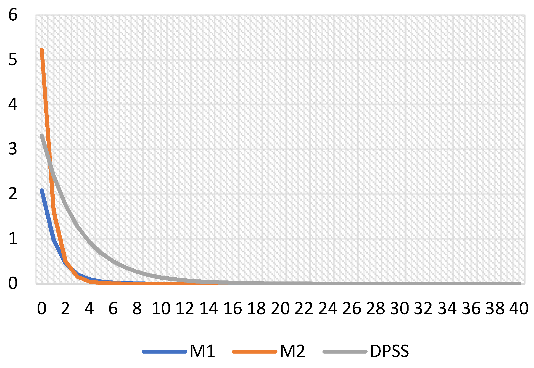
Global demand shock on oil price—Figure 1
A standard error positive shock (+1) was applied to all five models. However, the quadratic equations failed to solve for the oil price shocks with H1 and H2 models; therefore, they were not available. The DPSS takes the data up to 2011 when the oil prices were in the range of USD 100–110 per barrel for Brent oil. This contrasts with the recent low prices of 2019 and 2020. Brent was trading around USD 60 to 70 per barrel in 2019, with the extreme lows of USD 20 up to USD 50 in 2020. Negative prices happened in 2020 at the beginning of the lockdown, as physical stocks were in surplus, due to a lack of refineries to process them. At some point, the May future delivery was marked to USD −37.63 in April 2020. However, since the data in the model is on a quarterly basis, the short-lived negative prices had a smaller effect. The extreme price swings are reflected properly in the IRFs. A one standard error positive global demand shock was applied, and the responses were as expected. M2 with the 2020 prices showed the strongest response with over 5% per unit of SE of a demand shock. This is due to the volatile price swings in 2020, and the IRF responded as expected. The next two are DPSS (2011) and M1 (2019), which showed a modest 2% to 3% increase.
Figure 1.
Positive shock to Global Demand on Oil price.

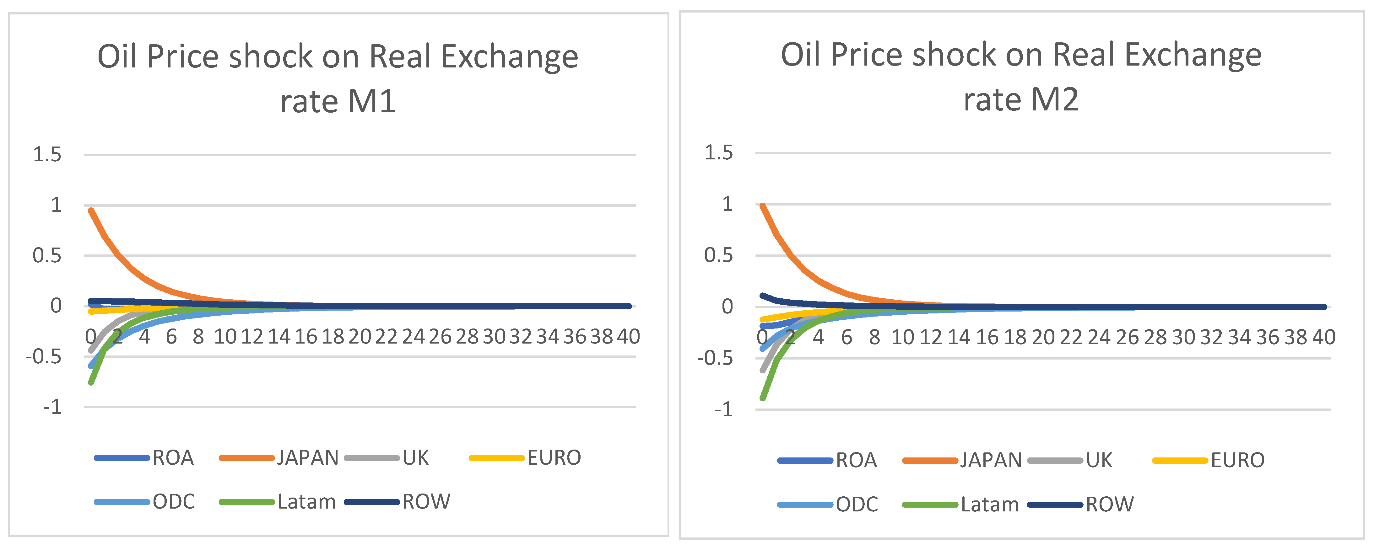
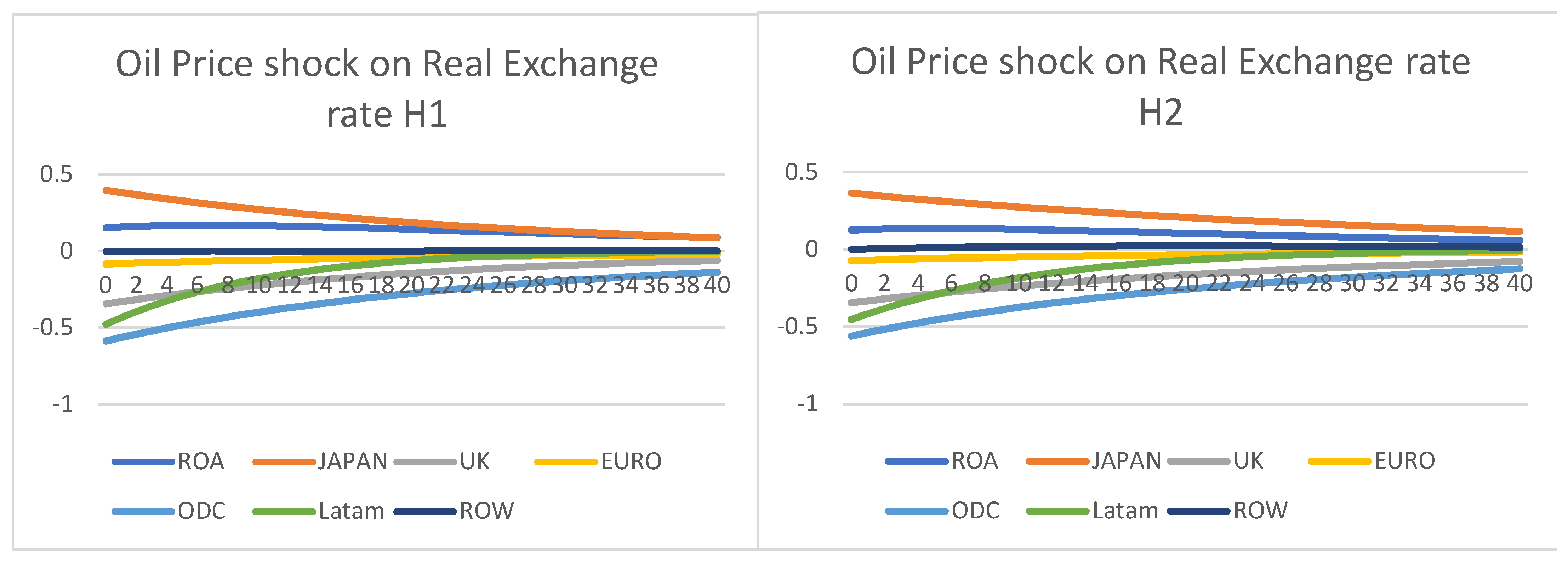
Oil Price shock on Real Exchange rate—Figure 2
Real exchange is not available for DPSS; therefore, they are not included for comparison. A positive oil price shock of one standard error was applied to all four models. For the DSGE–GVAR type models, both M1 and M2, as shown below, show that the real exchange rate tends to react strongly during the first few quarters to shocks, but often cycles back to steady-states a few quarters later. In particular, regions that are oil export-led, such as Latin America, Norway (ODC), and the UK, show that USD depreciate against them when oil prices increased. Conversely, big importers had their currencies depreciated against the USD, such as Japan (USD > JPY; therefore, showing a 1% increase of USD against JPY). Most regions, however, showed a low reaction, such as the Eurozone and ROW. This closely resembles what is observed in real life, as exchange rates tend to be stable around an equilibrium and should not drift, unless there is a strong economic situation, such as a currency devaluation. Including the 2020 data did not create much difference, although the effects were more pronounced for Latin America, but not significant. However, the DSGE-HP type models H1 and H2 showed IRFs that were not stable. This is shown in the graphs below, as none of the shocks apart from ROW returned to the steady-states; therefore, they are not stationary, nor stable enough to derive any conclusions. This is since using a HP filter diminished any meaningful cycles in the time-series; therefore, they have not captured any important features from history.
Figure 2.
Positive oil price shock on real exchange rates.


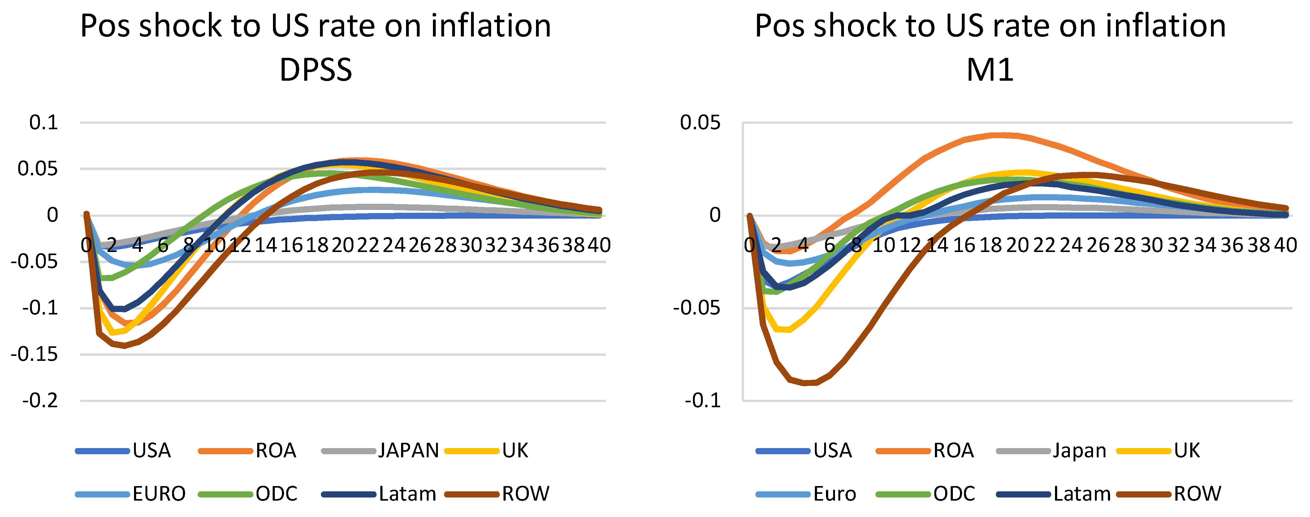
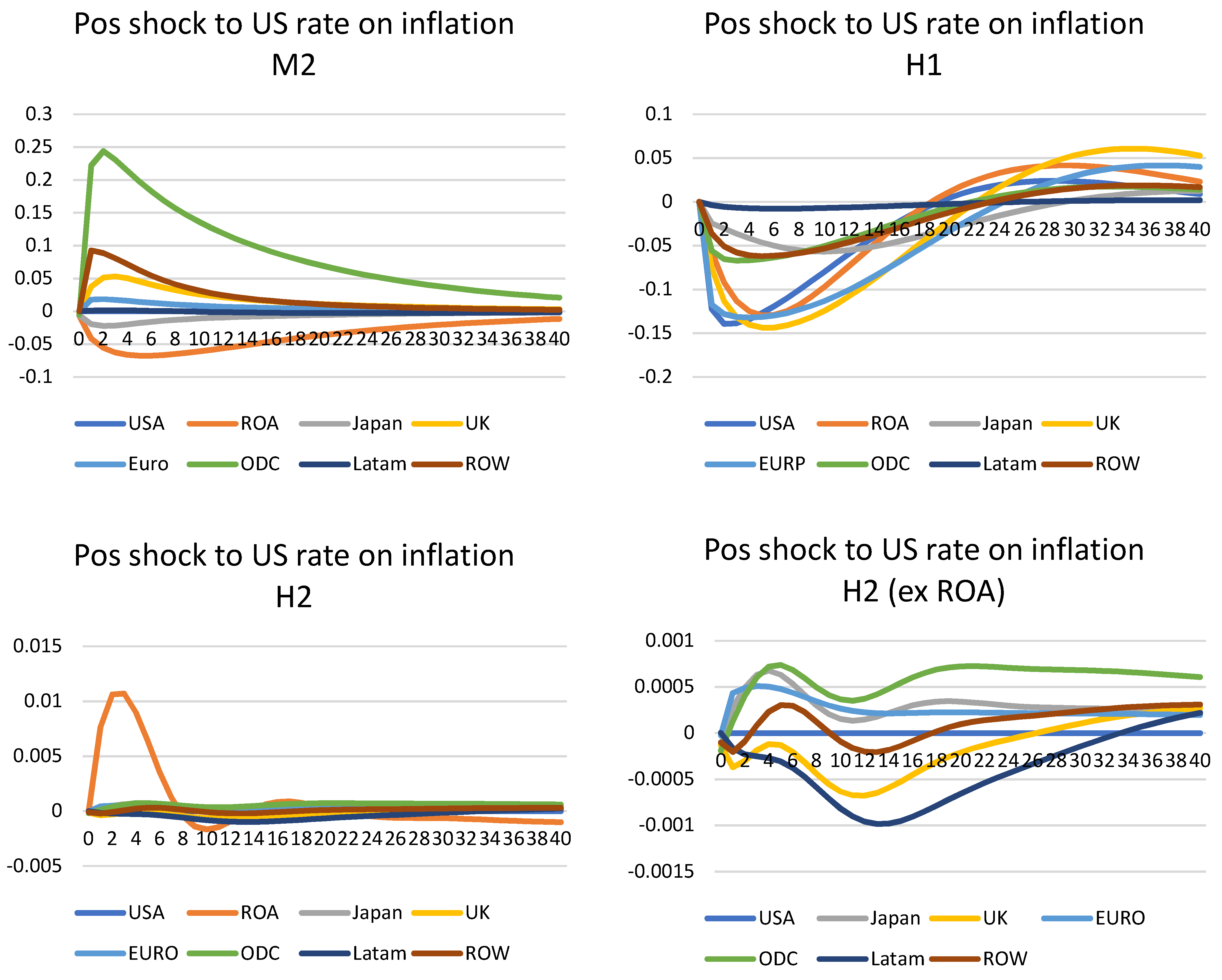
US monetary shock on inflation—Figure 3
All five models (DPSS, M1, M2, H1, and H2) are available for monetary shock and inflation; therefore, this shock was applied to all of them. Due to the lack of interest rate for Saudi Arabia, a global shock (i.e., shocking all countries) is not possible here. Instead, a US positive shock was used. A positive one standard error was applied. This is in the range of 0.22 basis points for the DPSS model to 0.15 for the M1, M2, H1, and H2 models. As expected, the US monetary policy shock depressed inflation in the US and other countries. This is consistent with the standard results in the literature,. Inflation soon returned to close to the steady-state within a few years for DPSS and M1. However, the case is a little more complicated for H1, where, although the model shows similar IRFs, they do not converge back to the steady-states after 40 quarters. This is similar to the above oil shock, where the Eigenvalues do not allow a stable solution.
Figure 3.
Positive monetary shock on inflation.


For DPSS and M1, by the fourth quarter, inflation for the US was −0.18% and output −0.50% below their steady-state values. This shape is similar to the paper of Smets and Wouters (2007, Figure 6) [21]. Their model showed that a monetary policy shock would cause interest rates to go up, then slowly return to zero, whereas the models here show initially raised interest rates, that are then quickly offset by the effects of the relatively sharp falls in inflation. On average after four quarters, inflation is lower. Relatively, US variables tend to return to their steady-state values when compared to other countries. This shows that a US monetary policy shock has a large global impact.
However, the cases for M2 and H2 are more complicated. The results from M2 show that the shocks cycle back to their steady-states relatively quickly. However, after including the data for 2020, the reaction of inflation to the interest raise is counterintuitive. Particularly for ODC, this showed a small but sharp spike in inflation. In general, except ROA and Japan, other areas showed inflation instead. This is probably as the majority of the countries have near or actual zero rates in their models. As such, any further increase would not show a significant decrease in inflation. Since the 2020 data show an abrupt decrease in interest rates globally and a strong decrease in inflation until the last quarter, the correlation between the two may be significant in the results here. The paradox of positive monetary shock and increase in inflation is a common problem in the VAR-shock literature. This was first noticed by Christiano et al. (1996) [22], but the ‘price puzzle’ was solved when introducing the commodity price index into the model.
One explanation has been attributed to the existence of a leading indicator for inflation, to which the central bank reacts and which is omitted from the VAR. The omission from the information set of a variable positively correlated with inflation and interest rates causes the VAR to be miss-specified; hence, the positive relation between inflation deviation and interest rates is observed. In theory, the extra channels from the international models, as well as global models of commodities, should capture the effect and inflation should show as negative instead. However, Pesaran et al. (2011) [14] also found this problem in their paper, and it could not be explained away by the extra time-series for different commodities. However, in the Covid-19 situation, the co-movement of lowering the interest rate and inflation affected the IRFs; therefore, the results were as shown below. For the DSGE–HP models, both show that their IRFs are unstable and did not converge to the steady-states. In particular, for H2, the majority of the models show indifference towards the shock, and their IRFs are not stable after 40 quarters.
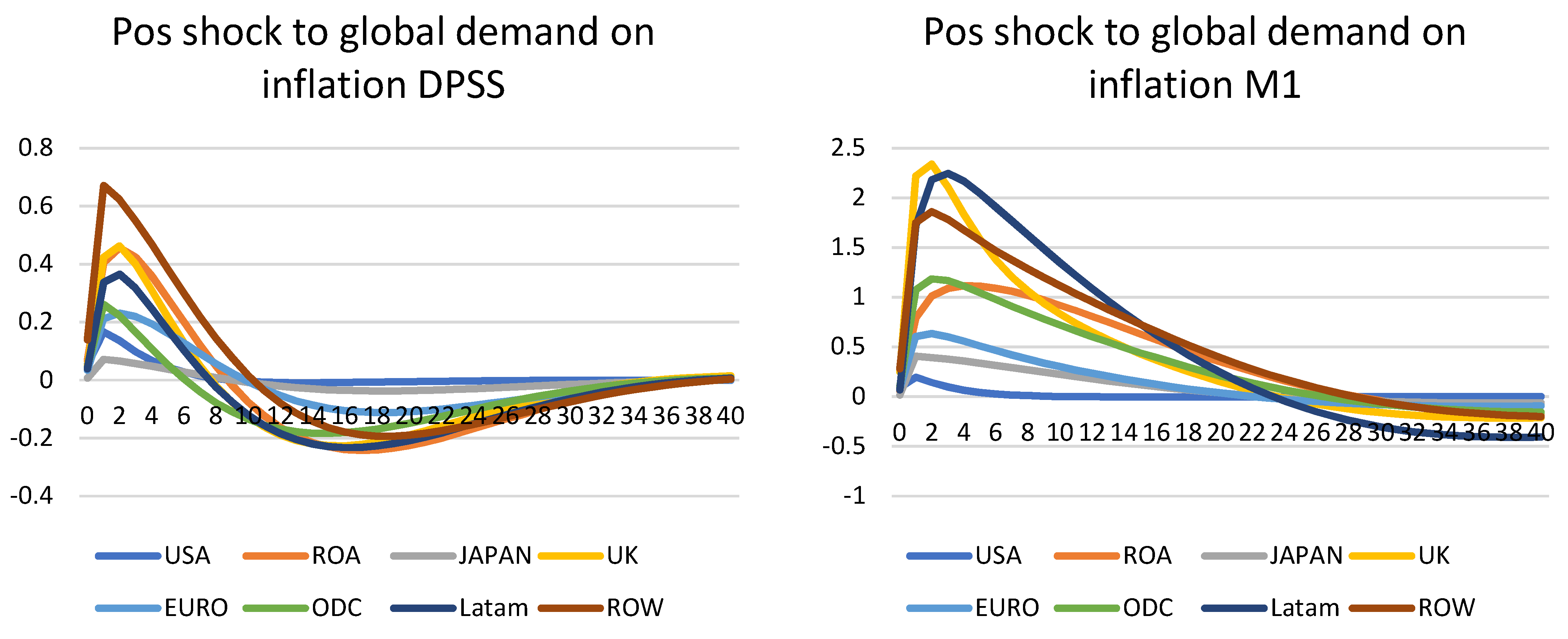
Global demand shock on inflation—Figure 4
All five models (DPSS, M1, M2, H1, and H2) are available for demand shock and inflation; therefore, this shock was applied to all of them. A positive one standard error global shock was used, i.e., all countries had their demand equation shocked and the effect on inflation was tested for below.
Figure 4.
Positive global demand on inflation.


For DPSS, M1, and H1, all show the expected shape of a sharp increase in inflation, before smoothly falling to the steady-states. The majority of the shocks also cycle back to their steady-states, although some remain after 40 quarters. In particular, the UK, USA, and ROA (including China) show a strong and sharp increase in inflation when there is a global demand shock. This is like the situation in 2021, when there was a sudden demand for the economy from the previous slump in 2020. This was also very similar to the inflation observed in the majority of countries in 2021, after the first two waves of the pandemic and the global lockdowns and travel restrictions. This is also similar to the 2020 models, but to a lesser extent. In this case, both models are distorted by the one-off increase in inflation seen in China due to the strict lockdowns. As such, both models have unusual shapes. Their IRFs are mostly stable and cycle back to the steady-states after 40 quarters. Taking ROA away, the models show a modest increase, before lowering to the steady-states. The effects are much less obvious than non-HP models, as their time-series lack the cyclical features after filtering.
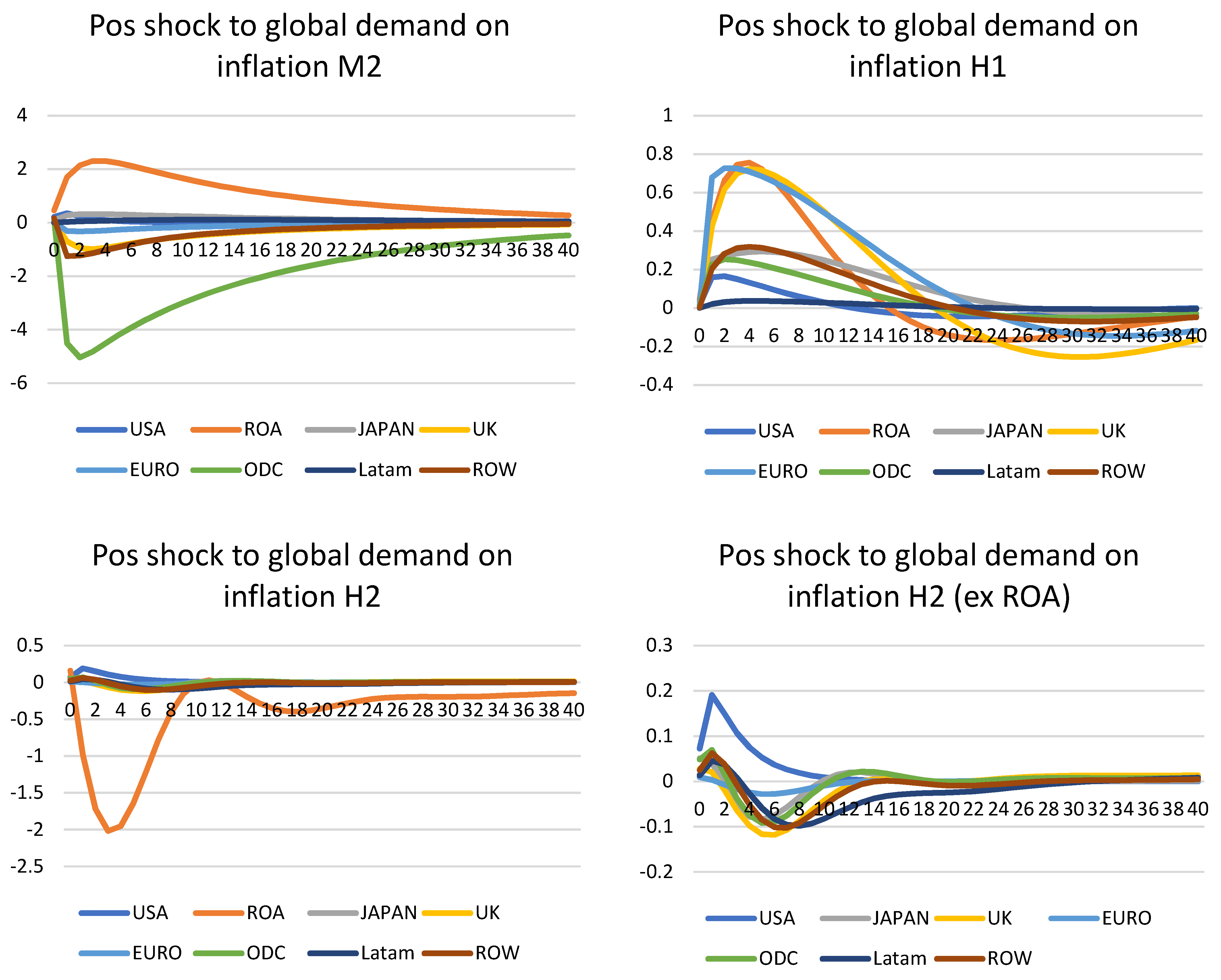
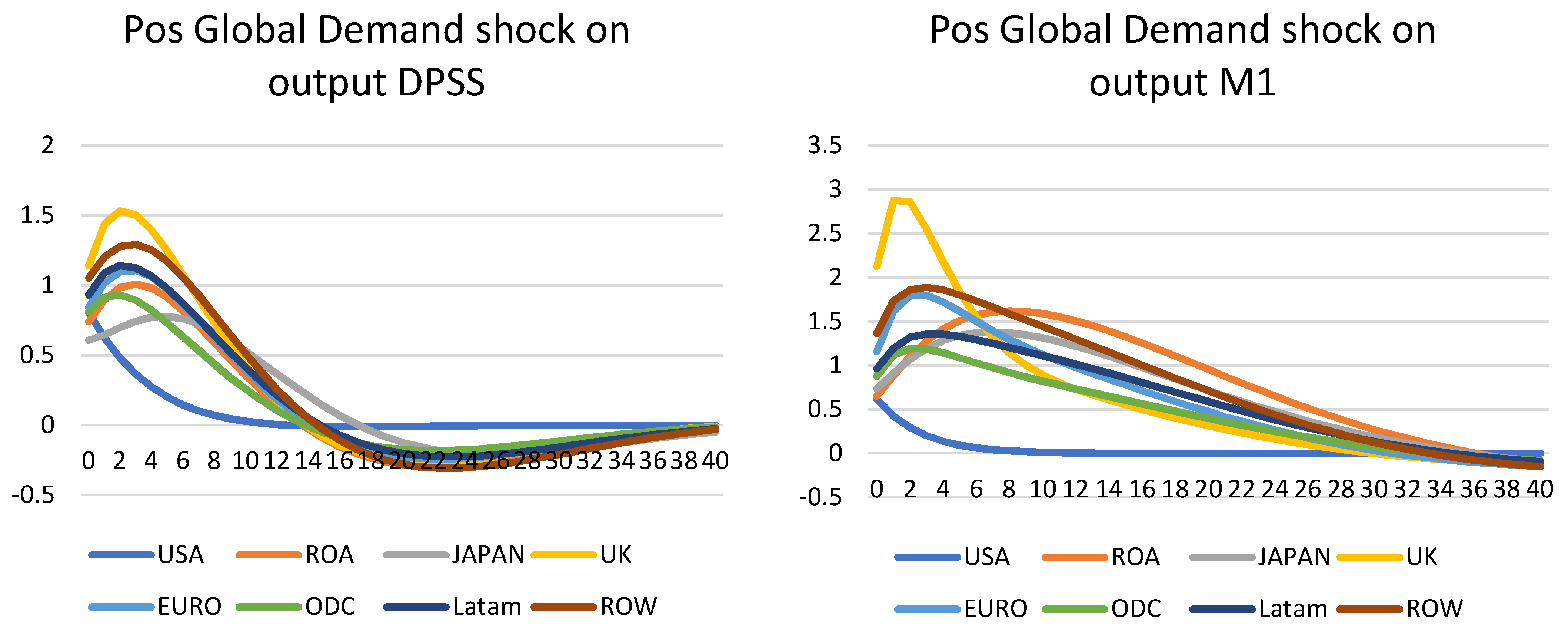
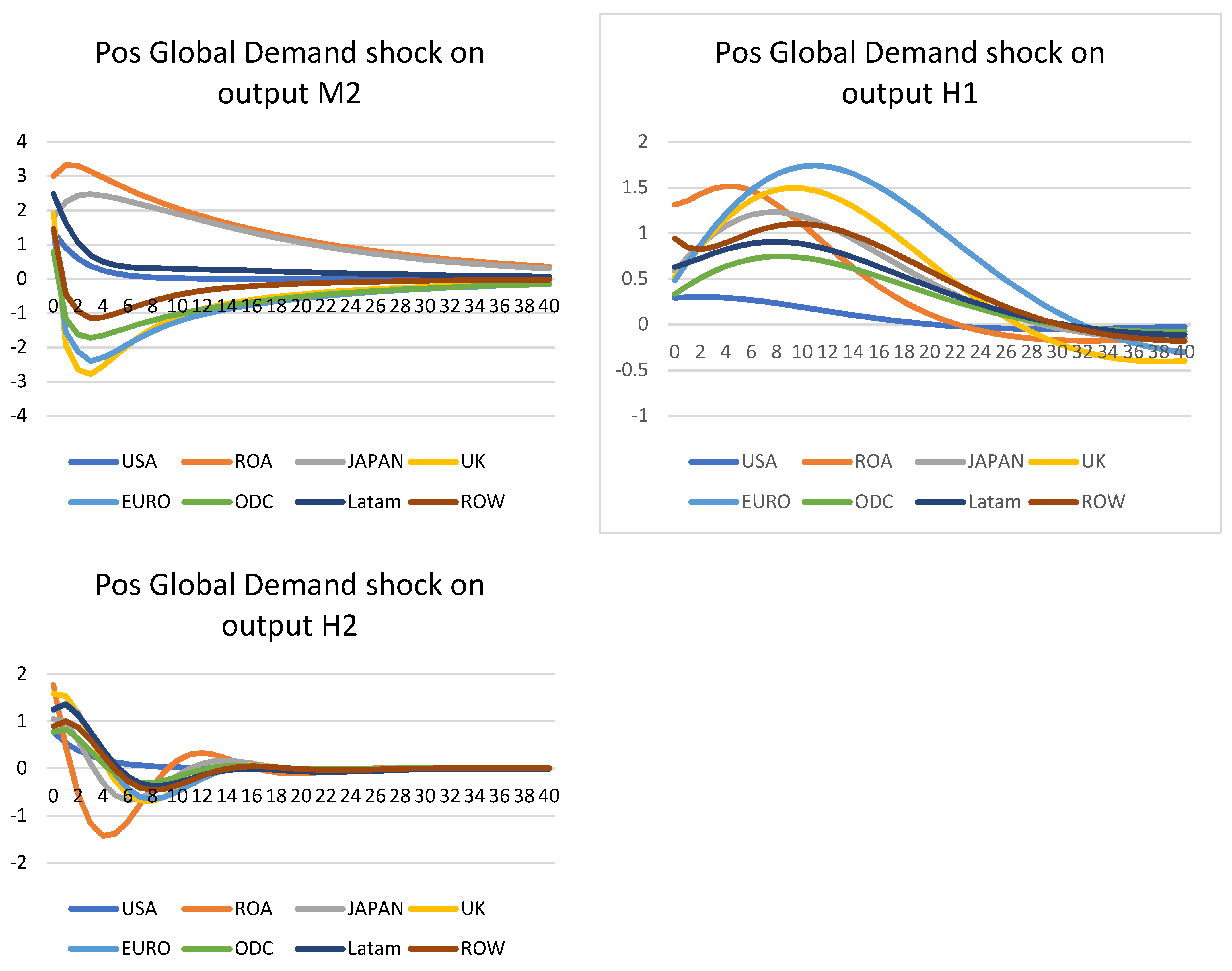
Global demand shock on output—Figure 5
All five models (DPSS, M1, M2, H1, and H2) are available for demand shock and output; therefore, this shock was applied to all of them. A positive one standard error global shock was used; i.e., all countries had their demand equation shocked and the effect on output was tested, as seen below. In general, the shapes are similar for the DPSS, DSGE-GVAR, and DSGE–HP type models. As expected, the output increased sharply upon impact, before settling down near or below the steady-states. The impact was in the range of 0.5% of output growth for Japan, to more than 1.5% for the UK in the second quarter. For the DPSS model, the shocks tended to revert after 4 to 5 years. This is due to the lower growth after the financial crisis and the beginning of the Euro crisis; therefore, the growth was the lowest among DPSS, M1, and H1. Prior to Covid-19, the growth was quite steady across all models; therefore, the M1 model showed the strongest growth and impact from a positive demand shock. The impact was also longer, lingering for 6 years. Similar shapes were also recorded for H1, but the peaks tended to be slower, and were only reached after 2–3 years. Given the sudden shock of the demand equation, the shocks should have moved quickly upon impact and decreased from the peak. As such, the DPSS and M1 provide better insights into actual growing paths. Including the 2020 data, both M2 and H2 models display a similar shape, but different paths of growth on output. Due to the extreme values in 2020, many region models had an initial boost, but immediately turned to negative growth once in the third quarter and after. The effect was particularly strong for M2 compared to H2, where the time-series were much smoother from the filter. The heavy infections in the US, ODC, and UK meant that lockdowns remained in place longer. As such, the economic impact was much stronger, and this affected their growth paths to negative, even after an initial increase. This, however, did not happen to ROA, for example; although China had initially discovered the virus, the impact was much weaker on the economy, as it experienced growth every year. As a result, the demand shock had a much stronger impact on ROA. This was, however, not captured in H2, as the sudden output gap (actual GDP minus HP steady-states) was much stronger than usual; therefore, actual growth was not predicted in this model.
Figure 5.
Positive global demand shock on output.


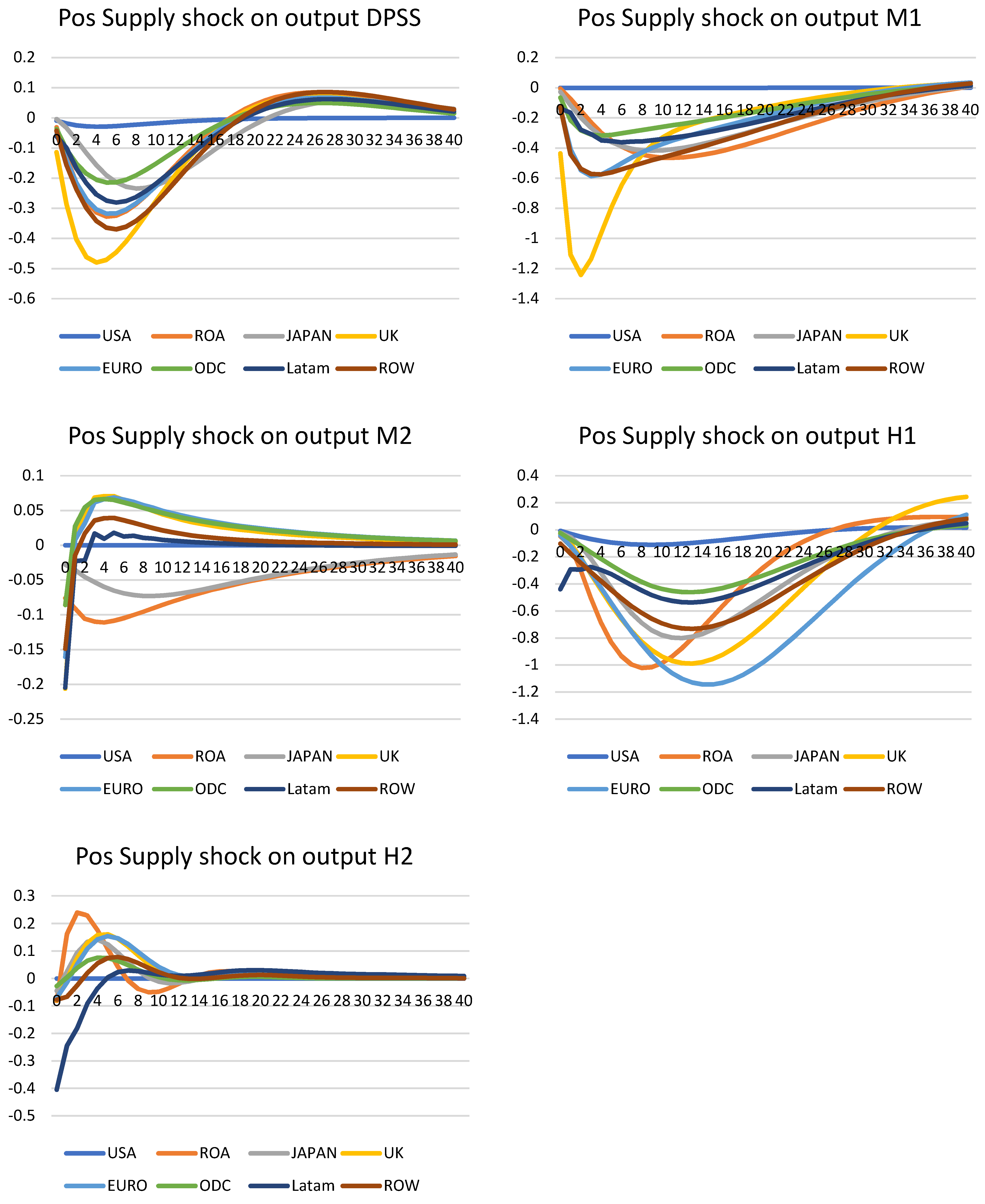
Supply shock on output—Figure 6
Next, a supply shock was applied to the output. This was done via a positive shock of one standard error to the Phillips curve. By definition, this shock causes inflation and interest rates to increase on impact, but here we are interested in the impact on output. The global supply shock also reduces output across all models; for the DPSS, with an average effect of −2.4% after four quarters. All regions suffered a decrease, except the US model. This was also true for the M1 and H1 models, although the updated data of M1 reflected a much stronger effect, with the UK in both models suffering the most. This was reflected in late 2021, with a double whammy of Brexit supply chain issues causing inflation and an increase of interest rate towards the end showing a similar effect. Regarding the pattern of dynamic adjustments, this model captured the deficiencies of importing for UK via the trade weight matrix and across trading partners. Both the DPSS and M1 also operated at a faster pace, as their effects slowed to steady-states after a few years. Qualitatively M1 also showed a similar pattern, but the speed was much slower and it took a few more years until it settled. However, for both H2 and M2 models, they exhibited a similar pattern of a sharp decrease, then a sharp bounce back to the steady-states. Perhaps not surprisingly, the extreme co-movements of decrease in inflation, interest rates, and output, and the sudden increase in inflation and output in the third and fourth quarters, reduced the impact of supply shocks to a sharp downturn, before recovering almost immediately. In this case, both models captured well the channels of supply shock transmission to output.
Figure 6.
Positive supply shock on output.

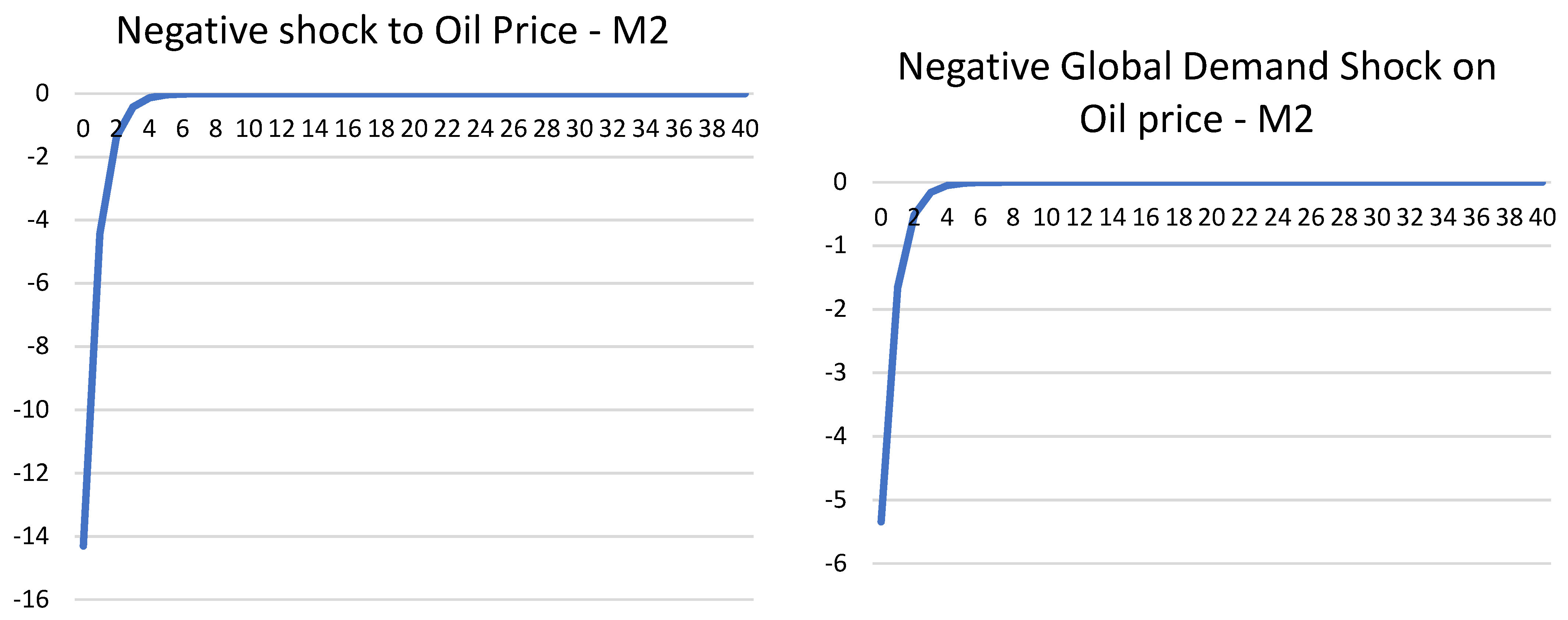
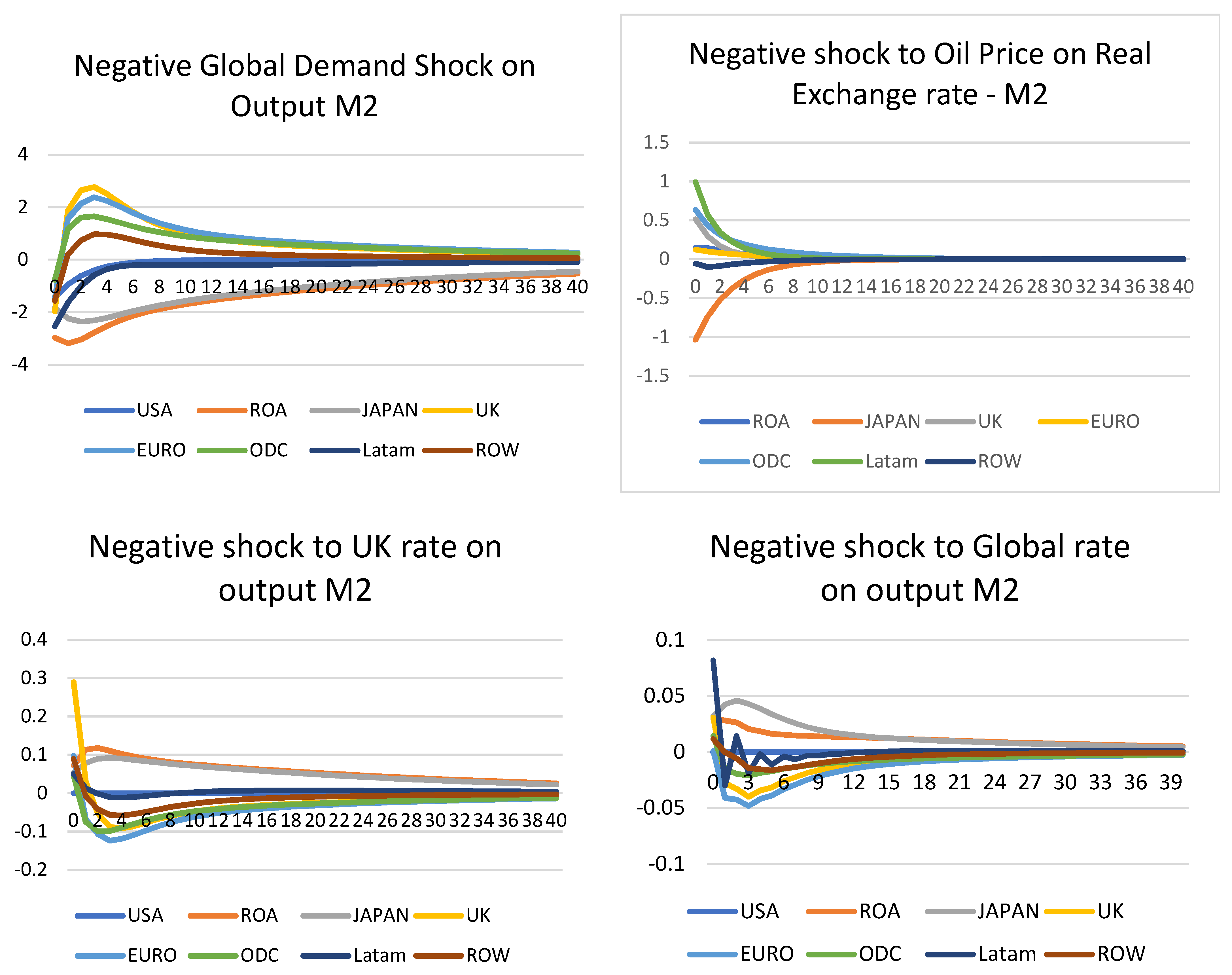
Additional negative shocks with M2—Figure 7
The shocks in the above sections form an exercise in understanding the impact of different shocks on the economy from a pre-and post-pandemic point of view. However, it is interesting to re-run some of the scenarios with negative shocks instead. As noted in the previous table, to stimulate a global interest rate shock, a completely closed model is required; therefore, the interest rate variable was approximated with repo for the Saudi Arabian model. In this section, for all models, there are eight regions (33 countries). Now that M2 contains all the pandemic data, it is expected to show a stronger impact on different variables given negative shocks. The first shock applied was a negative standard error to oil price. This was done for the oil price and the impact of oil price on real exchange rates. Not surprisingly, given the dramatic fall of the oil price in 2020, a 1 standard error drop in oil price shock saw a 14% drop on impact, although this sharply recovered to the steady-state levels. This is similar to the real oil price reaction in 2020, where it saw a sharp drop and recovery. Another shock was a negative global demand shock, and, similarly, this saw a drop in the oil price by about 5%. This is like the sudden emergence of the Omicron variant, where strict restrictions on travel were reintroduced in the fourth quarter of 2021 for most countries. This saw a sharp drop in oil price, from 5% to 10%, before recovering some losses. Another test considered, was a negative oil price shock to real exchange rates. This was as expected, as oil-importing regions such as Japan had appreciated against the USD, and oil-exporting currencies depreciated against the USD (USD was stronger; therefore, one dollar can exchange more currencies of Latam or ODC, hence, the increase). This was followed by a quick return to steady-states; therefore, this was as expected.
Figure 7.
Additional negative shocks to M2.


Lastly, an interesting exercise was performed on further rate decreases. First, in the UK scenario, where a sudden rate decrease happened, this would provide a small uplift to output for one quarter, before reversing the impact. If a global rate decrease shock happens, a similar effect is also felt. Here, the UK shock remained at a 0.3% increase in output for the global scenario. For all other countries, there was no discernible impact other than a weak growth in Japan and ROA. In both cases, the impact was about 0.05% to 0.025%, and soon reduced to steady-states. Zero and negative rates for Euro countries saw a minor decrease, and certainly had no growth impact.
9. Comparison with the DSGE Literature
DSGE dominates the macroeconomic modelling literature, and this is particularly the case with the majority of central banks using DSGE type models as their main models for policymaking; although, there are now other approaches being used such as time-series and semi-structural models (Central Banking, 2021) [23]. There are still difficulties in directly comparing VAR type models to DSGE, as both approaches are fundamentally different. The majority of DSGE models are also built for one to a few countries only, as there are relatively few works on an international multi-country scale. A possible comparison is often made via coefficients of the reduced-form VAR and a log-linearized version of the DSGE model and the impulse response functions.
The recent literature has made advances in comparing VAR and DSGE models. In some cases, direct comparison is possible. For example, Giacomini (2013) [24] discussed the method of mapping DSGE onto VAR models, by first transforming the DSGE model into a state-space model and then into an infinite order of VAR, and lastly into a finite order VAR. This is possible, as a simple non-linear DSGE model can be transformed into a log-linearized version that has an exact VAR(1) representation (An and Schorfheide, 2007) [25]. Often referred to as DSGE–VAR models, these are introduced to systematically mitigate the cross-coefficient constraints imposed on the VAR by the DSGE model. Depending on the specification of the DSGE models, approximations with VAR representation can be inexact, and, as such, there is often a discrepancy in terms of the forecasts or impulse response functions generated from the same data and approximated by DSGE–VAR models. As the approximates are not exact, there is a need to compare the outcome of a DSGE, DSGE-VAR, and an unrestricted VAR. For example, Lee (2018) [26] compared monetary policy effects from a small two-country open-economy model for South Korea and the US. In this case, the impulse responses of DSGE and DSGE-VAR were less similar. Forecasting performance was best with the VAR model, when estimated with the Bayesian technique. The inconsistent impulse response results in the fully structural DSGE, and reduced-form DSGE–VAR requires further investigations as to what kinds of misspecification or omitted variables exist.
Often the comparison exercise yields policy implications, as the outcome can be very different, depending on the model used, even as the discrepancy is limited as much as possible. There has, however, been a little comparison between large-scale DSGE models and large-scale VAR type models, such as GVAR. For example, there has been no work on translating a full GVAR model into unrestricted VAR and state–space model and lastly DSGE, in reverse order (there are works on DSGE-FAVAR, however; for example, Boivin and Giannoni(2006) [27] showed that it is possible to estimate a DSGE from a dynamic factor model. In Consolo, Favero, and Paccagnini (2009) [28], it was shown that DSGE-FAVAR can be an optimal forecasting model compared to the DSGE model itself).
Large scale DSGE models that are built for international and multi-country analysis, are primarily developed at central banks and policy institutions, and, as such, they are often not openly accessible. Some institutions have published working papers on their models. For example, medium and large-scale DSGE models at the European Central Bank New Area Wide Model (Christoffel et al., 2008 [29]; Karadi et al., 2018 [30]), COMPASS at Bank of England, and SIGMA from the Federal Reserve Board (Erceg et al., 2006) [31]. National central banks tend to have a smaller single country or region-based models built for capturing country-specific dynamics, such as MEDEA (Burriel et al., 2010) [32] and FiMOD (Stähler and Thomas, 2012) [33] for Spain, AINO 2.0 for Finland (Kilponen et al., 2016) [34], or GEAR for Germany (Gadatsch et al., 2016) [35]. Complete surveys on the macroeconomic models used were published by Kwok (2021) [36] and Welfe (2013) [37], and one can see that majority of models are tiny compared to the VAR or structural models, where the scale is often global. However, even if they belong to the same class of large-scale models, they differ in some dimensions. For example, many models are not always fully estimated (or calibrated) and even then, the information set and used for estimation varies substantially from one country model to another. Since the information and data set might change substantially over time, the parameter estimates and conclusions are not directly comparable, even within the DSGE literature. Meaningful cross-model comparison, therefore, requires a prudent approach, taking into consideration the data and model specification.
Considering the limitations of such a comparison, this section proceeds to consider some of the DSGE models in the literature, and a comparison is made, not with the purpose of cross-validation, but as an exercise to check the methodology used in this paper. Following the literature, two methods were used. The first is a partial comparison of the estimated coefficients in the three equations. This follows the approach in Lubik and Schorfheide (2004) [38], where the authors compared the estimated coefficients and posterior distribution of the DSGE and DSGE-VAR models. In our case, estimated coefficients of similar magnitude to the literature would be a boost to the methodology, as it would be evidence that the estimation of the DSGE-GVAR/DSGE-HP models is largely in line. The second method is performed via replicating the imposing response functions and comparing their shapes. This is done in a qualitative sense, where similar shapes from the models implied a correct estimation, as they are both generated from the New-Keynesian methodology. Further comparison of the speed of deviation closing to steady-states is further evidence that misspecification is not present in the model, as the opposite would imply the contrary.
To facilitate this comparison two major DSGE models in the literature were used. Replications were made using MMB (https://www.macromodelbase.com/ version MMB 3.1, Models used: US_SW07 and CA_LS07, accessed on 10 November 2021) i.e., Lubik and Schorfheide (2007) [39] and Smets and Wouters (2007) [21]. Both models are now considered to be the classic models in the New Keynesian literature, where a variant of the three-equation model is used. A rough comparison is possible with this paper’s GVAR–DSGE model, as both LS and SW are New Keynesian in nature. A straightforward comparison of the impulse response function is only possible for monetary shock. This is because both LS and SW have a simple Taylor type monetary rule. However, demand shock is impossible, as both models make use of microdata (such as hours worked) and price rigidities, such that the shocks are not directly comparable to the model in this paper.
Estimated coefficients and impulse responses
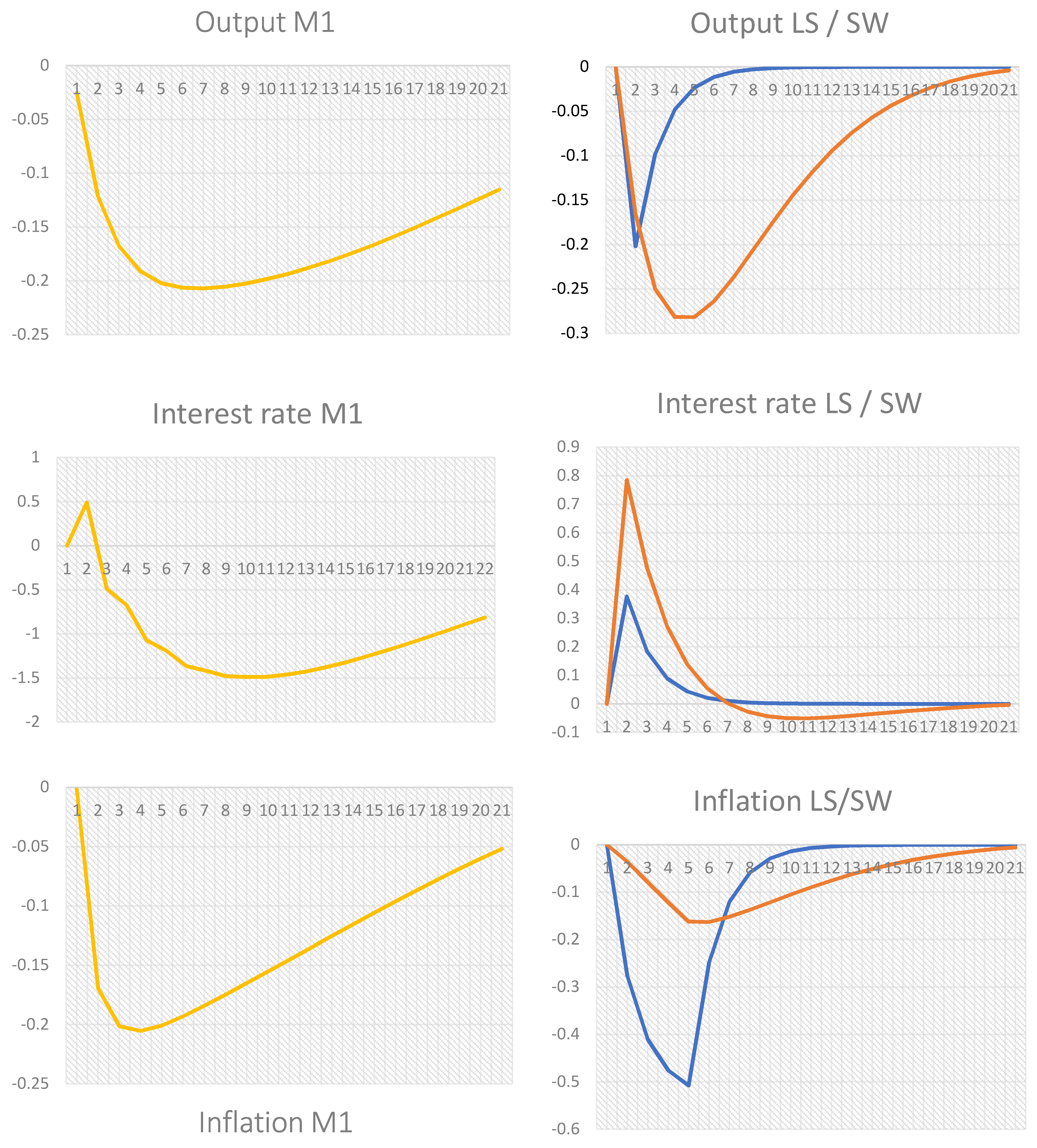
The below Table 3 summarizes the estimated coefficients for all models. The values are listed, where it was possible. The values are taken directly from the papers themselves where possible, or the MBB database if present. Lubik and Schorfheide (2007) [39] or LS, estimated a small-scale structural general equilibrium model of a small open economy using Bayesian methods. The LS model contains the countries of Australia, Canada, New Zealand, and the U.K. The model uses a generic Taylor-type rule, where monetary authority reacts in response to output, inflation, and exchange-rate movements. The model is comprised of an open-economy IS curve with exchange rates and Phillips curve; therefore, it is similar to the ones estimated in this paper. The posterior parameter estimate for the slope coefficient of the Phillips curve was 0.32, and the persistence in nominal interest rate was 0.69 (p. 1079). This is similar to the estimates from the DPSS model for similar periods (1980Q2/2011Q20), 0.33 and 0.65, correspondingly. Extending the data to 2019 and 2020 for M1, M2 produced estimates in a similar region, of 0.30/0.26 and 0.63/0.64. Figures from H1 and H2 were somewhat different, at 0.66/0.43 and 0.82/0.81. This explains the excessive responses from the impulse responses to different shocks. The SW model is similar but it uses both New Keynesian and neoclassical theories. It is often referred to as New Neoclassical Synthesis (NSS), as it combines both. For example, it uses both Phillips and Taylor curves in its models. Relative to previous models, SW has become the standard workhorse model, as it includes additional features that differentiate it from other NK models. For example, there are adjustment costs for investment, capacity utilization costs, habit persistence, and price and wage indexation. These features made it difficult to directly compare it to the models in this paper; however, it retains enough similar NK features with the Phillips, exchange rate, and Taylor equations. For the demand side, SW does not use an IS equation. The log-linearized version, instead, uses a combination of consumption and exogenous investment. As such, demand shocks are risk premium, exogenous spending, and investment-specific technology shocks, and no direct comparisons are possible. For monetary shocks, however, this is largely in line with LS and the Taylor rules employed in this paper. Typically, the interest rate depends on the last period’s interest rate, while gradually adjusting towards a target interest rate that depends on inflation and the gap between the output and its potential level. The coefficients for the Taylor model were estimated to be 0.96; therefore, it is much more aggressive than the other models. Looking at the impulse response of a positive one standard error shock, we can see that the interest rate reaction is much stronger than the expected 0.8; subsequently, inflation deviation rises much slower than in the LS model (orange lines for SW and blue for LS). Despite the differences in model specification, both LS and SW react similarly to monetary shock, except that the effect is stronger in SW. Comparing this to DSGE–GVAR models, we can see a similar pattern. Below are impulse response functions from the M1 model, and the results are averaged across regions; therefore, the results show an average response from the model.
In the examples here, illustrated in Figure 8, both replications for LS and SW are primarily for the US model and external linkages, if any. Therefore, averaged values from the DSGE-GVAR would give a similar interpretation, where the US dominates but is averaged out by external linkages. For the effect of a positive monetary policy shock on output, we can see that both M1 and SW/LS show a similar negative hump shape. The magnitude is also similar, between −0.2% and 0.3%. The biggest difference comes in the adjustment paths, where the LS model is much quicker than the other two, while both DSGE-GVAR and SW slowly adjust back to the steady-states within a few years. For interest rates, an adjustment was made for the DSGE–GVAR impulse response. The result was scaled by 10 times the original output from the M1 model. This is due to the low or even zero interest rates in many countries compared to the era of the 2007 models, where the interest rates were 5% to 6% on average before the crisis. This contrasts with the 0.5% average for the last few years. The shape remains the same, as it is only scaled up for comparison purposes. The initial response is largely the same, as all models react by increasing up to between 0.3% and 0.8%, before falling quickly. A similar pattern was observed for both SW and M1, where a negative effect was experienced, before converging back to the steady-states. Finally, all three models exhibited a similar reaction to inflation, where a drop of −0.2% to −0.5% was experienced, before increasing back to normal. The SW model had the largest value in its Taylor equation; therefore, this model has a stronger monetary authority in tracking the target, and, as such, it has the weakest reaction.
10. Conclusions
This paper developed a DSGE–GVAR multi-country model that is consistent with the New Keynesian framework. Furthermore, it tested the supply, demand, and monetary policy shocks, before and after the pandemic. The results from impulse responses clearly show that the DSGE–GVAR is better than fitting the DSGE model with just HP filtered values, which is the norm in the literature. The impact and sudden changes in 2020 caused some of the impulse responses to react strongly and unexpectedly. However, the majority of the shocks are in line with expectations. This is particularly true for the DSGE–GVAR models, unlike the HP filtered ones, where some of the models could not converge; therefore, indicating misspecification. This implies that the outcome is consistent with the framework. To reinforce the comparison with the wider literature, comparisons were also made with the DSGE literature, which showed that all models reacted similarly to monetary policy shocks, despite differences in the specification and the year.
Funding
This research received no external funding.
Institutional Review Board Statement
Not applicable.
Informed Consent Statement
Not applicable.
Data Availability Statement
For running GVAR model, the GVAR toolbox was used: https://sites.google.com/site/gvarmodelling/gvar-toolbox, accessed on 15 December 2021. For DSGE model replication, MMB was used: https://www.macromodelbase.com/ accessed on 15 December 2021.
Conflicts of Interest
The authors declare no conflict of interest.
Appendix A

Table A1.
VARX* Order of individual models p = lag order of domestic variables, q = lag order of foreign variables.
Table A1.
VARX* Order of individual models p = lag order of domestic variables, q = lag order of foreign variables.
| p | q | |
| ARGENTINA | 2 | 1 |
| AUSTRALIA | 1 | 1 |
| AUSTRIA | 1 | 1 |
| BELGIUM | 1 | 1 |
| BRAZIL | 2 | 1 |
| CANADA | 1 | 1 |
| CHINA | 2 | 1 |
| CHILE | 2 | 1 |
| FINLAND | 2 | 1 |
| FRANCE | 2 | 1 |
| GERMANY | 2 | 1 |
| INDIA | 2 | 1 |
| INDONESIA | 2 | 1 |
| ITALY | 2 | 1 |
| JAPAN | 2 | 1 |
| KOREA | 2 | 1 |
| MALAYSIA | 1 | 1 |
| MEXICO | 1 | 1 |
| NETHERLANDS | 2 | 1 |
| NORWAY | 2 | 1 |
| NEW ZEALAND | 2 | 1 |
| PERU | 2 | 1 |
| PHILIPPINES | 2 | 1 |
| SOUTH AFRICA | 2 | 1 |
| SAUDI ARABIA | 2 | 1 |
| SINGAPORE | 2 | 1 |
| SPAIN | 2 | 1 |
| SWEDEN | 2 | 1 |
| SWITZERLAND | 1 | 1 |
| THAILAND | 2 | 1 |
| TURKEY | 2 | 1 |
| UNITED KINGDOM | 2 | 1 |
| USA | 2 | 1 |
Table A2.
No. of Co-integrating Relationships for the Individual VARX* Models.
| Country | # Cointegrating Relations |
| ARGENTINA | 2 |
| AUSTRALIA | 5 |
| AUSTRIA | 3 |
| BELGIUM | 2 |
| BRAZIL | 2 |
| CANADA | 4 |
| CHINA | 2 |
| CHILE | 2 |
| FINLAND | 2 |
| FRANCE | 3 |
| GERMANY | 3 |
| INDIA | 2 |
| INDONESIA | 3 |
| ITALY | 2 |
| JAPAN | 2 |
| KOREA | 4 |
| MALAYSIA | 2 |
| MEXICO | 3 |
| NETHERLANDS | 2 |
| NORWAY | 5 |
| NEW ZEALAND | 3 |
| PERU | 4 |
| PHILIPPINES | 3 |
| SOUTH AFRICA | 3 |
| SAUDI ARABIA | 3 |
| SINGAPORE | 2 |
| SPAIN | 3 |
| SWEDEN | 2 |
| SWITZERLAND | 3 |
| THAILAND | 3 |
| TURKEY | 1 |
| UNITED KINGDOM | 1 |
| USA | 2 |
Table A3.
F-Statistics for the Serial Correlation Test of the VECMX* Residuals.
| Fcrit_0.05 | y | Dp | eq | ep | r | lr | ||
| ARGENTINA | F(4,140) | 2.44 | 1.16 | 0.98 | 1.05 | 0.75 | 0.89 | |
| AUSTRALIA | F(4,142) | 2.44 | 2.69 | 0.35 | 0.20 | 1.90 | 3.16 | 1.23 |
| AUSTRIA | F(4,144) | 2.43 | 3.86 | 1.34 | 3.29 | 3.18 | 0.68 | 7.25 |
| BELGIUM | F(4,145) | 2.43 | 2.47 | 1.96 | 1.48 | 5.03 | 5.36 | 1.92 |
| BRAZIL | F(4,141) | 2.44 | 2.77 | 2.28 | 0.63 | 1.09 | ||
| CANADA | F(4,143) | 2.43 | 1.24 | 2.20 | 1.80 | 3.85 | 2.93 | 1.08 |
| CHINA | F(4,141) | 2.44 | 3.97 | 4.28 | 1.09 | 6.00 | ||
| CHILE | F(4,140) | 2.44 | 1.12 | 2.29 | 1.27 | 2.14 | 0.34 | |
| FINLAND | F(4,140) | 2.44 | 1.37 | 4.98 | 2.33 | 1.52 | 1.80 | |
| FRANCE | F(4,138) | 2.44 | 1.39 | 3.50 | 0.34 | 0.26 | 2.31 | 3.02 |
| GERMANY | F(4,138) | 2.44 | 1.81 | 0.31 | 0.51 | 1.46 | 0.48 | 1.22 |
| INDIA | F(4,139) | 2.44 | 0.87 | 3.27 | 1.30 | 1.04 | 1.13 | 0.18 |
| INDONESIA | F(4,140) | 2.44 | 2.06 | 3.86 | 2.35 | 3.02 | ||
| ITALY | F(4,139) | 2.44 | 4.00 | 2.12 | 1.04 | 0.59 | 2.05 | 2.40 |
| JAPAN | F(4,139) | 2.44 | 1.65 | 0.20 | 0.53 | 4.27 | 1.37 | 2.39 |
| KOREA | F(4,137) | 2.44 | 3.41 | 4.00 | 2.00 | 2.27 | 0.47 | 1.61 |
| MALAYSIA | F(4,145) | 2.43 | 0.71 | 0.19 | 1.91 | 3.82 | 2.84 | |
| MEXICO | F(4,144) | 2.43 | 2.35 | 1.27 | 1.18 | 2.21 | ||
| NETHERLANDS | F(4,139) | 2.44 | 0.99 | 0.69 | 1.90 | 1.99 | 3.19 | 2.32 |
| NORWAY | F(4,136) | 2.44 | 2.36 | 1.64 | 1.25 | 1.43 | 1.99 | 3.50 |
| NEW ZEALAND | F(4,138) | 2.44 | 1.09 | 3.72 | 2.21 | 2.28 | 3.53 | 5.67 |
| PERU | F(4,139) | 2.44 | 2.56 | 4.69 | 3.02 | 6.10 | ||
| PHILIPPINES | F(4,139) | 2.44 | 4.10 | 1.29 | 0.42 | 0.07 | 3.11 | |
| SOUTH AFRICA | F(4,138) | 2.44 | 3.73 | 2.98 | 1.07 | 2.30 | 1.02 | 0.79 |
| SAUDI ARABIA | F(4,141) | 2.44 | 19.56 | 1.21 | 0.78 | |||
| SINGAPORE | F(4,140) | 2.44 | 2.32 | 2.21 | 2.12 | 1.48 | 3.86 | |
| SPAIN | F(4,138) | 2.44 | 4.07 | 3.01 | 1.01 | 1.80 | 1.63 | 1.45 |
| SWEDEN | F(4,139) | 2.44 | 0.99 | 4.96 | 4.09 | 1.89 | 2.03 | 3.07 |
| SWITZERLAND | F(4,144) | 2.43 | 5.93 | 4.06 | 1.37 | 2.00 | 1.01 | 1.68 |
| THAILAND | F(4,139) | 2.44 | 0.75 | 3.10 | 1.06 | 2.45 | 0.67 | |
| TURKEY | F(4,142) | 2.44 | 1.15 | 2.65 | 0.78 | 2.63 | ||
| UNITED KINGDOM | F(4,140) | 2.44 | 1.56 | 1.98 | 0.67 | 2.79 | 1.21 | 0.66 |
| USA | F(4,142) | 2.44 | 1.05 | 1.45 | 0.99 | 4.59 | 0.50 |
Table A4.
Average Pairwise Correlations—DSGE-GVAR (M1).
| Supply_Supply | Supply_Demand | Supply_MP | Supply_RE | Supply_Oil | Demand_Demand | Demand_MP | Demand_RE | Demand_Oil | MP_MP | MP_RE | MP_Oil | RE_RE | RE_Oil | Oil_Oil | |
| OIL | 1 | ||||||||||||||
| USA | 0.31 | 0.11 | 0.22 | 0.04 | −0.03 | 0.04 | 0.05 | −0.07 | 0.42 | 0.27 | −0.05 | 0.10 | |||
| CHINA | 0.02 | 0.01 | −0.08 | −0.07 | −0.01 | 0.07 | 0.07 | 0.00 | 0.02 | 0.09 | 0.03 | 0.20 | −0.04 | 0.01 | |
| JAPAN | 0.57 | 0.22 | 0.04 | 0.02 | −0.05 | 0.09 | 0.13 | 0.02 | 0.14 | 0.26 | −0.03 | −0.05 | −0.15 | 0.26 | |
| UNITED KINGDOM | 0.62 | 0.25 | 0.04 | 0.03 | −0.18 | 0.23 | 0.05 | 0.02 | −0.14 | 0.29 | 0.00 | 0.09 | −0.01 | −0.27 | |
| AUSTRIA | 0.62 | 0.24 | 0.02 | 0.04 | −0.15 | 0.19 | 0.04 | 0.01 | −0.11 | 0.34 | 0.00 | 0.19 | −0.02 | 0.11 | |
| BELGIUM | 0.62 | 0.25 | 0.03 | 0.03 | −0.18 | 0.21 | 0.05 | 0.03 | −0.13 | 0.32 | 0.00 | 0.00 | −0.01 | 0.10 | |
| FINLAND | 0.62 | 0.25 | 0.04 | 0.03 | −0.17 | 0.05 | 0.01 | −0.05 | −0.13 | 0.30 | 0.01 | 0.01 | −0.02 | 0.16 | |
| FRANCE | 0.63 | 0.25 | 0.05 | 0.03 | −0.15 | 0.13 | 0.08 | 0.00 | −0.05 | 0.31 | 0.00 | −0.05 | −0.03 | 0.06 | |
| GERMANY | 0.07 | 0.03 | 0.00 | 0.00 | 0.42 | 0.01 | 0.02 | −0.01 | 0.08 | 0.30 | 0.00 | 0.02 | −0.01 | 0.13 | |
| ITALY | 0.44 | 0.15 | 0.06 | 0.03 | 0.10 | 0.07 | 0.11 | 0.03 | 0.05 | 0.28 | 0.05 | −0.09 | 0.01 | −0.21 | |
| NETHERLANDS | 0.51 | 0.18 | 0.03 | 0.03 | 0.01 | 0.06 | 0.02 | 0.00 | −0.12 | 0.31 | 0.00 | 0.09 | −0.05 | −0.18 | |
| SPAIN | 0.62 | 0.24 | 0.05 | 0.03 | −0.09 | 0.06 | 0.05 | 0.02 | −0.19 | 0.23 | 0.04 | −0.09 | 0.03 | −0.12 | |
| NORWAY | 0.53 | 0.20 | 0.03 | 0.01 | −0.08 | 0.00 | 0.00 | 0.03 | −0.02 | 0.11 | 0.01 | −0.02 | 0.04 | −0.23 | |
| SWEDEN | 0.62 | 0.25 | 0.04 | 0.03 | −0.20 | 0.21 | 0.05 | 0.02 | −0.14 | 0.24 | 0.01 | 0.10 | 0.05 | −0.31 | |
| SWITZERLAND | 0.62 | 0.25 | 0.03 | 0.03 | −0.18 | 0.04 | 0.05 | 0.02 | 0.05 | 0.10 | −0.02 | 0.09 | 0.00 | 0.16 | |
| AUSTRALIA | 0.60 | 0.24 | 0.03 | 0.02 | −0.11 | 0.05 | 0.05 | −0.02 | 0.04 | 0.12 | 0.00 | −0.01 | 0.09 | −0.46 | |
| CANADA | 0.60 | 0.24 | 0.05 | 0.02 | −0.09 | 0.10 | 0.10 | −0.03 | 0.03 | 0.24 | −0.04 | 0.11 | 0.09 | −0.50 | |
| NEW ZEALAND | 0.62 | 0.24 | 0.04 | 0.03 | −0.16 | 0.06 | 0.09 | 0.03 | −0.04 | 0.09 | 0.01 | −0.04 | 0.09 | −0.33 | |
| ARGENTINA | 0.10 | 0.04 | 0.04 | −0.01 | −0.06 | −0.03 | −0.04 | 0.00 | 0.09 | 0.07 | 0.03 | 0.01 | −0.04 | −0.08 | |
| BRAZIL | 0.47 | 0.18 | 0.00 | 0.00 | −0.12 | 0.08 | 0.04 | 0.05 | −0.03 | 0.01 | 0.03 | −0.07 | 0.06 | −0.19 | |
| CHILE | 0.29 | 0.07 | 0.06 | 0.02 | 0.04 | 0.01 | 0.05 | 0.05 | −0.09 | 0.06 | 0.00 | −0.09 | 0.09 | −0.18 | |
| MEXICO | 0.16 | 0.04 | 0.00 | 0.07 | −0.17 | 0.00 | 0.10 | −0.03 | 0.13 | 0.09 | 0.01 | 0.01 | 0.11 | −0.47 | |
| PERU | −0.03 | 0.00 | 0.00 | 0.01 | 0.09 | 0.04 | 0.05 | −0.01 | −0.06 | −0.08 | −0.03 | 0.00 | 0.01 | 0.14 | |
| INDONESIA | −0.06 | −0.03 | −0.02 | −0.01 | −0.02 | 0.11 | 0.10 | −0.01 | −0.05 | 0.12 | 0.01 | 0.07 | −0.01 | −0.10 | |
| KOREA | 0.62 | 0.24 | 0.05 | 0.03 | −0.18 | 0.01 | −0.04 | −0.02 | 0.11 | 0.13 | 0.02 | −0.04 | 0.04 | −0.31 | |
| MALAYSIA | 0.62 | 0.25 | 0.02 | 0.02 | −0.16 | 0.07 | 0.07 | −0.05 | 0.05 | 0.06 | −0.01 | 0.04 | 0.09 | −0.08 | |
| PHILIPPINES | 0.62 | 0.25 | 0.03 | 0.03 | −0.19 | 0.05 | −0.02 | −0.03 | 0.10 | 0.13 | −0.01 | −0.02 | 0.06 | −0.08 | |
| SINGAPORE | 0.56 | 0.23 | 0.05 | 0.02 | −0.05 | 0.10 | −0.03 | −0.01 | −0.12 | 0.22 | 0.00 | 0.07 | 0.06 | −0.20 | |
| THAILAND | 0.62 | 0.25 | 0.02 | 0.02 | −0.13 | 0.00 | 0.00 | −0.04 | 0.04 | 0.20 | −0.04 | 0.11 | 0.03 | 0.14 | |
| INDIA | −0.13 | −0.06 | −0.11 | −0.01 | 0.02 | 0.02 | −0.09 | 0.01 | 0.04 | 0.10 | 0.02 | −0.13 | 0.03 | 0.28 | |
| SOUTH AFRICA | 0.18 | 0.05 | 0.10 | 0.01 | 0.14 | 0.06 | 0.02 | 0.03 | −0.06 | 0.09 | 0.01 | −0.18 | 0.01 | −0.12 | |
| SAUDI ARABIA | −0.13 | −0.05 | −0.08 | −0.01 | 0.04 | 0.00 | 0.06 | 0.01 | 0.11 | −0.04 | 0.37 | ||||
| TURKEY | 0.49 | 0.21 | −0.02 | 0.02 | −0.20 | 0.16 | −0.01 | 0.03 | 0.03 | 0.03 | 0.02 | −0.13 | 0.02 | 0.01 |
Table A5.
Country Weights DSGE-GVAR.
| Country | Dp_c | y_c | r_c | ep_c |
| ARGENTINA | 0.010 | 0.010 | 0.010 | 0.010 |
| AUSTRALIA | 0.015 | 0.015 | 0.015 | 0.015 |
| AUSTRIA | 0.006 | 0.006 | 0.006 | 0.006 |
| BELGIUM | 0.007 | 0.007 | 0.007 | 0.007 |
| BRAZIL | 0.035 | 0.035 | 0.035 | 0.035 |
| CANADA | 0.024 | 0.024 | 0.024 | 0.024 |
| CHINA | 0.134 | 0.134 | 0.136 | 0.134 |
| CHILE | 0.004 | 0.004 | 0.004 | 0.004 |
| FINLAND | 0.003 | 0.003 | 0.004 | 0.003 |
| FRANCE | 0.039 | 0.039 | 0.039 | 0.039 |
| GERMANY | 0.054 | 0.054 | 0.054 | 0.054 |
| INDIA | 0.059 | 0.059 | 0.059 | 0.059 |
| INDONESIA | 0.016 | 0.016 | 0.016 | 0.016 |
| ITALY | 0.035 | 0.035 | 0.035 | 0.035 |
| JAPAN | 0.081 | 0.081 | 0.082 | 0.081 |
| KOREA | 0.024 | 0.024 | 0.025 | 0.024 |
| MALAYSIA | 0.007 | 0.007 | 0.007 | 0.007 |
| MEXICO | 0.028 | 0.028 | 0.029 | 0.028 |
| NETHERLANDS | 0.012 | 0.012 | 0.012 | 0.012 |
| NORWAY | 0.005 | 0.005 | 0.005 | 0.005 |
| NEW ZEALAND | 0.002 | 0.002 | 0.002 | 0.002 |
| PERU | 0.004 | 0.004 | 0.004 | 0.004 |
| PHILIPPINES | 0.006 | 0.006 | 0.006 | 0.006 |
| SOUTH AFRICA | 0.009 | 0.009 | 0.009 | 0.009 |
| SAUDI ARABIA | 0.011 | 0.011 | 0.011 | |
| SINGAPORE | 0.004 | 0.004 | 0.004 | 0.004 |
| SPAIN | 0.026 | 0.026 | 0.027 | 0.026 |
| SWEDEN | 0.006 | 0.006 | 0.006 | 0.006 |
| SWITZERLAND | 0.006 | 0.006 | 0.006 | 0.006 |
| THAILAND | 0.010 | 0.010 | 0.010 | 0.010 |
| TURKEY | 0.018 | 0.018 | 0.018 | 0.018 |
| UNITED KINGDOM | 0.040 | 0.040 | 0.041 | 0.040 |
| USA | 0.260 | 0.260 | 0.263 | 0.260 |
Table A6.
Regional Weights DSGE-GVAR.
| Region | Country | Dp_c | y_c | r_c | ep_c |
| japan | japan | 1.00 | 1.00 | 1.00 | 1.00 |
| la | arg | 0.12 | 0.12 | 0.12 | 0.12 |
| la | bra | 0.43 | 0.43 | 0.43 | 0.43 |
| la | chl | 0.05 | 0.05 | 0.05 | 0.05 |
| la | mex | 0.35 | 0.35 | 0.35 | 0.35 |
| la | per | 0.05 | 0.05 | 0.05 | 0.05 |
| odc | nor | 0.08 | 0.08 | 0.08 | 0.08 |
| odc | swe | 0.11 | 0.11 | 0.11 | 0.11 |
| odc | switz | 0.10 | 0.10 | 0.10 | 0.10 |
| odc | austlia | 0.26 | 0.26 | 0.26 | 0.26 |
| odc | can | 0.41 | 0.41 | 0.41 | 0.41 |
| odc | nzld | 0.04 | 0.04 | 0.04 | 0.04 |
| restworld | safrc | 0.24 | 0.24 | 0.33 | 0.24 |
| restworld | sarbia | 0.28 | 0.28 | 0.28 | |
| restworld | turk | 0.48 | 0.48 | 0.67 | 0.48 |
| uk | uk | 1 | 1 | 1 | 1 |
| usa | usa | 1 | 1 | 1 | 1 |
| euro | austria | 0.032 | 0.032 | 0.032 | 0.032 |
| euro | bel | 0.038 | 0.038 | 0.038 | 0.038 |
| euro | fin | 0.019 | 0.019 | 0.019 | 0.019 |
| euro | france | 0.214 | 0.214 | 0.214 | 0.214 |
| euro | germ | 0.295 | 0.295 | 0.295 | 0.295 |
| euro | italy | 0.190 | 0.190 | 0.190 | 0.190 |
| euro | neth | 0.067 | 0.067 | 0.067 | 0.067 |
| euro | spain | 0.145 | 0.145 | 0.145 | 0.145 |
| restasia | indns | 0.061 | 0.061 | 0.061 | 0.061 |
| restasia | kor | 0.094 | 0.094 | 0.094 | 0.094 |
| restasia | mal | 0.026 | 0.026 | 0.026 | 0.026 |
| restasia | phlp | 0.022 | 0.022 | 0.022 | 0.022 |
| restasia | sing | 0.017 | 0.017 | 0.017 | 0.017 |
| restasia | thai | 0.038 | 0.038 | 0.038 | 0.038 |
| restasia | india | 0.226 | 0.226 | 0.226 | 0.226 |
| restasia | china | 0.517 | 0.517 | 0.517 | 0.517 |
Table A7.
Oil model-DSGE-GVAR.
| Country | Yvar | Xvar1 | coeffs1 | se1 | t-ratio1 | se_NW1 | t-ratioNW1 | LM_CHSQ(4) | GRsq |
| OIL | poil_c | poil_c(-1) | 0.47 | 0.08 | 5.66 | 0.12 | 3.89 | 7.11 | 0.40 |
Table A8.
Phillips Curve-DSGE-GVAR.
| Country | coeffs1 | coeffs2 | coeffs3 | t-ratio1 | t-ratio2 | t-ratio3 |
| USA | 0.06 | 0.91 | 0.14 | 0.55 | 4.77 | 3.09 |
| CHINA | 0.47 | 0.21 | 0.14 | 5.51 | 2.74 | 1.58 |
| JAPAN | 0.00 | 0.99 | 0.02 | |||
| UNITED KINGDOM | 0.16 | 0.79 | 0.12 | 1.67 | 6.51 | 4.36 |
| AUSTRIA | 0.06 | 0.93 | 0.05 | |||
| BELGIUM | 0.04 | 0.95 | 0.11 | |||
| FINLAND | 0.35 | 0.62 | 0.04 | 4.05 | 5.16 | 2.65 |
| FRANCE | 0.09 | 0.86 | 0.06 | 0.76 | 6.24 | 2.27 |
| GERMANY | 0.04 | 0.00 | 0.09 | |||
| ITALY | 0.18 | 0.81 | 0.00 | |||
| NETHERLANDS | 0.18 | 0.57 | 0.07 | 1.95 | 3.89 | 2.18 |
| SPAIN | 0.08 | 0.91 | 0.04 | 0.69 | 6.08 | 1.78 |
| NORWAY | 0.06 | 0.93 | 0.03 | |||
| SWEDEN | 0.04 | 0.87 | 0.15 | 0.36 | 5.64 | 3.38 |
| SWITZERLAND | 0.28 | 0.71 | 0.11 | |||
| AUSTRALIA | 0.06 | 0.78 | 0.19 | 0.54 | 3.97 | 2.49 |
| CANADA | 0.16 | 0.74 | 0.08 | 1.69 | 6.67 | 2.88 |
| NEW ZEALAND | 0.00 | 0.99 | 0.10 | |||
| ARGENTINA | 0.01 | 0.98 | 0.00 | |||
| BRAZIL | 0.25 | 0.74 | 0.13 | |||
| CHILE | 0.30 | 0.65 | 0.00 | |||
| MEXICO | 0.41 | 0.58 | 0.00 | |||
| PERU | 0.26 | 0.49 | 0.00 | |||
| INDONESIA | 0.38 | 0.59 | 0.00 | |||
| KOREA | 0.19 | 0.80 | 0.14 | |||
| MALAYSIA | 0.03 | 0.96 | 0.04 | |||
| PHILIPPINES | 0.29 | 0.70 | 0.16 | |||
| SINGAPORE | 0.15 | 0.70 | 0.05 | 1.59 | 3.72 | 1.88 |
| THAILAND | 0.18 | 0.81 | 0.02 | |||
| INDIA | 0.13 | 0.50 | 0.00 | |||
| SOUTH AFRICA | 0.07 | 0.92 | 0.00 | |||
| SAUDI ARABIA | 0.35 | 0.29 | 0.00 | |||
| TURKEY | 0.11 | 0.74 | 0.27 | 0.93 | 1.64 | 1.28 |
Table A9.
IS Curve-DSGE-GVAR.
| Country | coeffs1 | coeffs2 | coeffs3 | coeffs4 | coeffs5 | coeffs6 |
| USA | 0.69 | −0.01 | 0.01 | |||
| CHINA | 0.64 | −0.43 | 0.43 | 0.00 | 0.00 | 0.22 |
| JAPAN | 0.71 | −0.34 | 0.34 | −0.05 | 0.05 | 0.27 |
| UNITED KINGDOM | 0.29 | −0.49 | 0.49 | 0.09 | −0.09 | 1.08 |
| AUSTRIA | 0.18 | −0.49 | 0.49 | −0.14 | 0.14 | 1.06 |
| BELGIUM | 0.15 | −0.13 | 0.13 | −0.11 | 0.11 | 1.00 |
| FINLAND | 0.09 | 0.00 | 0.00 | 0.12 | −0.12 | 1.32 |
| FRANCE | 0.27 | 0.00 | 0.00 | −0.04 | 0.04 | 0.73 |
| GERMANY | 0.06 | −0.07 | 0.07 | −0.05 | 0.05 | 1.27 |
| ITALY | 0.08 | 0.00 | 0.00 | −0.21 | 0.21 | 0.57 |
| NETHERLANDS | 0.07 | −0.03 | 0.03 | 0.00 | 0.00 | 0.82 |
| SPAIN | 0.24 | 0.00 | 0.00 | −0.17 | 0.17 | 0.71 |
| NORWAY | −0.09 | 0.00 | 0.00 | −0.06 | 0.06 | 0.52 |
| SWEDEN | 0.04 | −0.32 | 0.32 | 0.08 | −0.08 | 1.21 |
| SWITZERLAND | 0.01 | 0.00 | 0.00 | −0.03 | 0.03 | 0.79 |
| AUSTRALIA | 0.19 | 0.00 | 0.00 | −0.01 | 0.01 | 0.53 |
| CANADA | 0.51 | 0.00 | 0.00 | −0.02 | 0.02 | 0.81 |
| NEW ZEALAND | 0.03 | 0.00 | 0.00 | −0.04 | 0.04 | 0.54 |
| ARGENTINA | 0.46 | 0.00 | 0.00 | 0.00 | 0.00 | 0.64 |
| BRAZIL | 0.09 | −0.01 | 0.01 | −0.04 | 0.04 | 1.20 |
| CHILE | 0.20 | −0.29 | 0.29 | −0.32 | 0.32 | 1.10 |
| MEXICO | 0.32 | −0.15 | 0.15 | −0.02 | 0.02 | 1.01 |
| PERU | 0.57 | 0.00 | 0.00 | −0.02 | 0.02 | 0.32 |
| INDONESIA | 0.64 | 0.00 | 0.00 | −0.11 | 0.11 | 1.23 |
| KOREA | 0.46 | 0.00 | 0.00 | 0.01 | −0.01 | 0.39 |
| MALAYSIA | 0.20 | 0.00 | 0.00 | 0.00 | 0.00 | 1.52 |
| PHILIPPINES | 0.72 | 0.00 | 0.00 | 0.04 | −0.04 | 0.63 |
| SINGAPORE | 0.06 | −0.11 | 0.11 | 0.12 | −0.12 | 1.46 |
| THAILAND | 0.67 | 0.00 | 0.00 | 0.04 | −0.04 | 1.38 |
| INDIA | 0.27 | 0.00 | 0.00 | −0.12 | 0.12 | 0.00 |
| SOUTH AFRICA | 0.56 | 0.00 | 0.00 | −0.12 | 0.12 | 0.57 |
| SAUDI ARABIA | 0.50 | 0.00 | −0.15 | 0.15 | 0.34 | |
| TURKEY | −0.01 | −0.22 | 0.22 | −0.15 | 0.15 | 1.40 |
Table A10.
Taylor rule-DSGE-GVAR.
| Country | coeffs1 | coeffs2 | coeffs3 | se1 | se2 | se3 | t-ratio1 | t-ratio2 | t-ratio3 |
|---|---|---|---|---|---|---|---|---|---|
| USA | 0.92 | 0.15 | 0.02 | 0.03 | 0.05 | 0.01 | 34.94 | 3.00 | 1.77 |
| CHINA | 0.85 | 0.03 | 0.02 | 0.07 | 0.03 | 0.02 | 12.53 | 1.10 | 1.16 |
| JAPAN | 0.91 | 0.16 | 0.00 | 0.03 | 0.05 | 34.97 | 3.28 | ||
| UNITED KINGDOM | 0.83 | 0.28 | 0.00 | 0.03 | 0.05 | 26.16 | 5.47 | ||
| AUSTRIA | 0.96 | 0.00 | 0.03 | 0.03 | 0.06 | 31.14 | 0.50 | ||
| BELGIUM | 0.94 | 0.11 | 0.03 | 0.03 | 0.06 | 0.01 | 30.14 | 1.81 | 2.15 |
| FINLAND | 0.90 | 0.20 | 0.02 | 0.03 | 0.05 | 0.01 | 34.26 | 4.22 | 2.43 |
| FRANCE | 0.84 | 0.24 | 0.03 | 0.04 | 0.06 | 0.01 | 23.69 | 4.08 | 2.17 |
| GERMANY | 0.85 | 0.10 | 0.03 | 0.04 | 0.07 | 0.01 | 20.95 | 1.47 | 2.98 |
| ITALY | 0.84 | 0.23 | 0.03 | 0.04 | 0.09 | 0.02 | 19.86 | 2.71 | 1.30 |
| NETHERLANDS | 0.95 | 0.02 | 0.04 | 0.03 | 0.06 | 0.01 | 28.82 | 0.27 | 3.40 |
| SPAIN | 0.92 | 0.09 | 0.01 | 0.04 | 0.07 | 0.02 | 24.23 | 1.24 | 0.57 |
| NORWAY | 0.84 | 0.11 | 0.04 | 0.07 | 0.06 | 0.03 | 12.79 | 1.70 | 1.41 |
| SWEDEN | 0.92 | 0.10 | 0.01 | 0.03 | 0.05 | 0.02 | 27.49 | 1.87 | 0.69 |
| SWITZERLAND | 0.49 | 0.03 | 0.07 | 0.06 | 0.04 | 0.01 | 8.73 | 0.67 | 6.50 |
| AUSTRALIA | 0.42 | 0.12 | 0.14 | 0.05 | 0.03 | 0.02 | 9.04 | 4.43 | 8.66 |
| CANADA | 0.80 | 0.29 | 0.00 | 0.04 | 0.05 | 22.38 | 5.49 | ||
| NEW ZEALAND | 0.49 | 0.33 | 0.18 | 0.05 | 0.04 | 0.04 | 9.33 | 7.66 | 5.11 |
| ARGENTINA | −0.27 | 0.28 | 0.00 | 0.12 | 0.12 | −2.27 | 2.34 | ||
| BRAZIL | −0.61 | 1.51 | 0.00 | 0.14 | 0.22 | −4.37 | 6.88 | ||
| CHILE | 0.40 | 0.63 | 0.01 | 0.11 | 0.18 | 0.04 | 3.56 | 3.49 | 0.33 |
| MEXICO | 0.01 | 0.37 | 0.06 | 0.04 | 0.02 | 0.02 | 0.33 | 18.22 | 2.48 |
| PERU | −0.19 | 0.39 | 0.04 | 0.18 | 0.11 | 0.22 | −1.03 | 3.52 | 0.19 |
| INDONESIA | 0.67 | 0.22 | 0.10 | 0.04 | 0.04 | 0.02 | 16.27 | 4.88 | 4.69 |
| KOREA | 0.72 | 0.20 | 0.09 | 0.06 | 0.06 | 0.03 | 12.40 | 3.35 | 3.16 |
| MALAYSIA | 0.54 | 0.00 | 0.01 | 0.07 | 0.02 | 7.96 | 0.15 | ||
| PHILIPPINES | 0.73 | 0.22 | 0.01 | 0.05 | 0.05 | 0.02 | 15.57 | 4.60 | 0.59 |
| SINGAPORE | 0.97 | 0.06 | 0.02 | 0.02 | 0.04 | 0.01 | 47.89 | 1.42 | 3.62 |
| THAILAND | 0.81 | 0.13 | 0.00 | 0.04 | 0.07 | 18.10 | 1.95 | ||
| INDIA | 0.49 | 0.16 | 0.00 | 0.12 | 0.08 | 4.01 | 2.06 | ||
| SOUTH AFRICA | 0.64 | 0.14 | 0.06 | 0.05 | 0.04 | 0.01 | 12.63 | 3.12 | 7.06 |
| TURKEY | 0.64 | 0.12 | 0.09 | 0.06 | 0.05 | 0.03 | 10.98 | 2.51 | 2.74 |
Table A11.
Real Exchange equation DSGE-GVAR.
| Country | coeffs1 | coeffs2 | coeffs3 | se1 | se2 | t-ratio1 | t-ratio2 |
|---|---|---|---|---|---|---|---|
| USA | 0.01 | 0.00 | 3.24 | ||||
| CHINA | 0.79 | −0.79 | 1.00 | 0.05 | 0.05 | 15.07 | 15.07 |
| JAPAN | 0.73 | −0.73 | 1.00 | 0.06 | 0.06 | 12.43 | 12.43 |
| UNITED KINGDOM | 0.58 | −0.58 | 1.00 | 0.07 | 0.07 | 7.98 | 7.98 |
| AUSTRIA | 0.55 | −0.55 | 1.00 | 0.07 | 0.07 | 7.94 | 7.94 |
| BELGIUM | 0.66 | −0.66 | 1.00 | 0.06 | 0.06 | 10.60 | 10.60 |
| FINLAND | 0.58 | −0.58 | 1.00 | 0.07 | 0.07 | 8.69 | 8.69 |
| FRANCE | 0.39 | −0.39 | 1.00 | 0.08 | 0.08 | 5.02 | 5.02 |
| GERMANY | 0.49 | −0.49 | 1.00 | 0.07 | 0.07 | 6.62 | 6.62 |
| ITALY | 0.49 | −0.49 | 1.00 | 0.07 | 0.07 | 6.55 | 6.55 |
| NETHERLANDS | 0.73 | −0.73 | 1.00 | 0.06 | 0.06 | 12.52 | 12.52 |
| SPAIN | 0.84 | −0.84 | 1.00 | 0.05 | 0.05 | 17.99 | 17.99 |
| NORWAY | 0.42 | −0.42 | 1.00 | 0.08 | 0.08 | 5.64 | 5.64 |
| SWEDEN | 0.71 | −0.71 | 1.00 | 0.06 | 0.06 | 12.19 | 12.19 |
| SWITZERLAND | 0.49 | −0.49 | 1.00 | 0.07 | 0.07 | 6.70 | 6.70 |
| AUSTRALIA | 0.59 | −0.59 | 1.00 | 0.07 | 0.07 | 8.94 | 8.94 |
| CANADA | 0.84 | −0.84 | 1.00 | 0.04 | 0.04 | 19.33 | 19.33 |
| NEW ZEALAND | 0.35 | −0.35 | 1.00 | 0.07 | 0.07 | 4.90 | 4.90 |
| ARGENTINA | 0.54 | −0.54 | 1.00 | 0.07 | 0.07 | 7.46 | 7.46 |
| BRAZIL | 0.28 | −0.28 | 1.00 | 0.09 | 0.09 | 3.15 | 3.15 |
| CHILE | 0.52 | −0.52 | 1.00 | 0.07 | 0.07 | 7.04 | 7.04 |
| MEXICO | 0.69 | −0.69 | 1.00 | 0.06 | 0.06 | 11.84 | 11.84 |
| PERU | 0.59 | −0.59 | 1.00 | 0.07 | 0.07 | 8.64 | 8.64 |
| INDONESIA | 0.48 | −0.48 | 1.00 | 0.07 | 0.07 | 6.88 | 6.88 |
| KOREA | 0.73 | −0.73 | 1.00 | 0.05 | 0.05 | 14.37 | 14.37 |
| MALAYSIA | 0.53 | −0.53 | 1.00 | 0.07 | 0.07 | 7.60 | 7.60 |
| PHILIPPINES | 0.71 | −0.71 | 1.00 | 0.06 | 0.06 | 11.80 | 11.80 |
| SINGAPORE | 0.66 | −0.66 | 1.00 | 0.06 | 0.06 | 10.36 | 10.36 |
| THAILAND | 0.56 | −0.56 | 1.00 | 0.07 | 0.07 | 8.02 | 8.02 |
| INDIA | 0.29 | −0.29 | 1.00 | 0.08 | 0.08 | 3.66 | 3.66 |
| SOUTH AFRICA | 0.68 | −0.68 | 1.00 | 0.06 | 0.06 | 11.56 | 11.56 |
| SAUDI ARABIA | 0.82 | −0.82 | 1.00 | 0.05 | 0.05 | 16.54 | 16.54 |
| TURKEY | 0.20 | −0.20 | 1.00 | 0.10 | 0.10 | 1.98 | 1.98 |
References
- Carabenciov, I.; Freedman, C.; Garcia-Saltos, M.R.; Laxton, M.D.; Kamenik, M.O.; Manchev, M.P. Gpm6: The Global Projection Model with 6 Regions; International Monetary Fund: Washington, DC, USA, 2013. [Google Scholar]
- Eichenbaum, M.S.; Rebelo, S.; Trabandt, M. The Macroeconomics of Epidemics. Rev. Financ. Stud. 2021, 34, 5149–5187. [Google Scholar] [CrossRef]
- Chudik, A.; Mohaddes, K.; Pesaran, M.H.; Raissi, M.; Rebucci, A. A counterfactual economic analysis of Covid-19 using a threshold augmented multi-country model. J. Int. Money Financ. 2021, 119, 102477. [Google Scholar] [CrossRef] [PubMed]
- Dées, S.; Pesaran, M.H.; Smith, L.V.; Smith, R.P. Constructing Multi-Country Rational Expectations Models. Oxf. Bull. Econ. Stat. 2013, 76, 812–840. [Google Scholar] [CrossRef]
- Smith, R.P. The GVAR approach to structural modelling. In The GVAR Handbook: Structure and Applications of a Macro Model of the Global Economy for Policy Analysis; Oxford University Press: Oxford, UK, 2013; pp. 56–69. [Google Scholar]
- Di Mauro, F.; Pesaran, M.H. (Eds.) The GVAR Handbook: Structure and Applications of a Macro Model of the Global Economy for Policy Analysis; OUP Oxford: Oxford, UK, 2013. [Google Scholar]
- Dées, S.; Pesaran, M.H.; Smith, L.V.; Smith, R.P. Identification of New Keynesian Phillips Curves from a Global Perspective. J. Money Crédit. Bank. 2009, 41, 1481–1502. [Google Scholar] [CrossRef] [Green Version]
- Pesaran, M.H. Time Series and Panel Data Econometrics; Oxford University Press (OUP): Oxford, UK, 2015. [Google Scholar]
- Pesaran, M.H.; Schuermann, T.; Weiner, S.M. Modeling Regional Interdependencies Using a Global Error-Correcting Macroeconometric Model. J. Bus. Econ. Stat. 2004, 22, 129–162. [Google Scholar] [CrossRef]
- Johansen, S. Testing weak exogeneity and the order of cointegration in UK money demand data. J. Policy Model. 1992, 14, 313–334. [Google Scholar] [CrossRef]
- Granger, C.W.; Lin, J.L. Causality in the long run. Econom. Theory 1995, 11, 530–536. [Google Scholar]
- Smith, L.; Galesi, A. GVAR Toolbox 2.0; University of Cambridge, Judge Business School, 2014; Available online: https://sites.google.com/site/gvarmodelling/gvar-toolbox/download (accessed on 13 December 2021).
- Quandt, R.E. The estimation of the parameters of a linear regression system obeying two separate regimes. J. Am. Stat. Assoc. 1958, 53, 873–880. [Google Scholar] [CrossRef]
- Pesaran, M.H.; Smith, R.P. Beyond the Dsge Straitjacket1. Manch. Sch. 2011, 79, 5–16. [Google Scholar] [CrossRef] [Green Version]
- Ploberger, W.; Krämer, W. The Cusum Test with Ols Residuals. Economet 1992, 60, 271. [Google Scholar] [CrossRef]
- Nyblom, J. Testing for the constancy of parameters over time. J. Am. Stat. Assoc. 1989, 84, 223–230. [Google Scholar] [CrossRef]
- Quandt, R.E. Tests of the hypothesis that a linear regression system obeys two separate regimes. J. Am. Stat. Assoc. 1960, 55, 324–330. [Google Scholar] [CrossRef]
- Andrews, D.W.K.; Ploberger, W. Optimal Tests when a Nuisance Parameter is Present Only Under the Alternative. Econometrica 1994, 62, 1383. [Google Scholar] [CrossRef]
- Canova, F.; Sala, L. Back to square one: Identification issues in DSGE models. J. Monetary Econ. 2009, 56, 431–449. [Google Scholar] [CrossRef] [Green Version]
- Koop, G.; Potter, S.M. Time varying VARs with inequality restrictions. J. Econ. Dyn. Control 2011, 35, 1126–1138. [Google Scholar] [CrossRef] [Green Version]
- Smets, F.; Wouters, R. Shocks and Frictions in US Business Cycles: A Bayesian DSGE Approach. Am. Econ. Rev. 2007, 97, 586–606. [Google Scholar] [CrossRef] [Green Version]
- Christiano, L.J.; Eichenbaum, M.; Evans, C. The Effects of Monetary Policy Shocks: Evidence from the Flow of Funds. Rev. Econ. Stat. 1996, 78, 16. [Google Scholar] [CrossRef]
- Central Banking. “Benchmarking 2021, Advanced Economies Draw on Wider Range of Models”. 2021. Available online: https://www.centralbanking.com/benchmarking/economics/7907091/advanced-economies-draw-on-wider-range-of-models (accessed on 12 October 2021).
- Giacomini, R. The relationship between DSGE and VAR models. In VAR Models in Macroeconomics–New Developments and Applications: Essays in Honor of Christopher A Sims; Emerald Group Publishing Limited: Bingley, UK, 2013. [Google Scholar]
- An, S.; Schorfheide, F. Bayesian Analysis of DSGE Models. Econ. Rev. 2007, 26, 113–172. [Google Scholar] [CrossRef] [Green Version]
- Lee, K.Y. A Comparison Analysis of Monetary Policy Effect Under an Open Economy Model. East Asian Econ. Rev. 2018, 22, 141–176. [Google Scholar] [CrossRef]
- Boivin, J.; Giannoni, M.P. Has Monetary Policy Become More Effective? Rev. Econ. Stat. 2006, 88, 445–462. [Google Scholar] [CrossRef] [Green Version]
- Consolo, A.; Favero, C.A.; Paccagnini, A. On the statistical identification of DSGE models. J. Econ. 2009, 150, 99–115. [Google Scholar] [CrossRef] [Green Version]
- Christoffel, K.; Coenen, G.; Warne, A. The New Area-Wide Model of the Euro Area; ECB working paper: Frankfurt, Germany, 2008. [Google Scholar]
- Karadi, P.; Schmidt, S.; Warne, A. The New Area-Wide Model ii: An Updated Version of the Ecb’s Micro-Founded Model for Forecasting and Policy Analysis with a Financial Sector; European Central Bank: Frankurt, Germany, 2018. [Google Scholar]
- Erceg, C.; Guerrieri, L.; Gust, C. SIGMA: A New Open Economy; IFDP Discussion Paper No.835; 2006. Available online: https://www.google.com.hk/url?sa=t&rct=j&q=&esrc=s&source=web&cd=&ved=2ahUKEwjdzqmk1fT3AhUp6mEKHcH8DC8QFnoECAIQAQ&url=https%3A%2F%2Fwww.federalreserve.gov%2Fpubs%2Fifdp%2F2005%2F835%2Fifdp835r.pdf&usg=AOvVaw2quRYrPH-jku9AqZYlJOKp (accessed on 15 December 2021).
- Burriel, P.; Fernández-Villaverde, J.; Rubio-Ramírez, J.F. MEDEA: A DSGE model for the Spanish economy. SERIEs 2010, 1, 175–243. [Google Scholar] [CrossRef]
- Stähler, N.; Thomas, C. FiMod—A DSGE model for fiscal policy simulations. Econ. Model. 2012, 29, 239–261. [Google Scholar] [CrossRef] [Green Version]
- Kilponen, J.; Orjasniemi, S.; Ripatti, A.; Verona, F. The Aino 2.0 model. In Bank of Finland Research Discussion Paper; 2016; Volume 16, Available online: https://papers.ssrn.com/sol3/papers.cfm?abstract_id=2795479 (accessed on 15 December 2021).
- Gadatsch, N.; Hauzenberger, K.; Stähler, N. Fiscal policy during the crisis: A look on Germany and the Euro area with GEAR. Econ. Model. 2016, 52, 997–1016. [Google Scholar] [CrossRef]
- Kwok, J. Macroeconometric Models for Portfolio Management; Vernon Press: Malaga, Spain, 2021. [Google Scholar]
- Welfe, W. Macroeconometric Models; Springer: Berlin, Germany, 2013. [Google Scholar] [CrossRef]
- Lubik, T.A.; Schorfheide, F. Testing for Indeterminacy: An Application to U.S. Monetary Policy. Am. Econ. Rev. 2004, 94, 190–217. [Google Scholar] [CrossRef] [Green Version]
- Lubik, T.A.; Schorfheide, F. Do central banks respond to exchange rate movements? A structural investigation. J. Monetary Econ. 2007, 54, 1069–1087. [Google Scholar] [CrossRef] [Green Version]
Figure 8.
Comparison of M1 and LS/SW. Color blue is for Lubik and Schorfheide (2007) [39] and orange is for Smets and Wouters (2007) [21].

Table 1.
Average pairwise correlations of shocks.
| Demand | Monetary | Real Ex | Oil | |
|---|---|---|---|---|
| Supply | 0.160 | 0.026 | 0.018 | −0.069 |
| Demand | - | 0.039 | 0.000 | 0.001 |
| Monetary | - | - | 0.003 | 0.009 |
Table 2.
Summary of estimated models.
| Model Name | Type | Period | Countries | Number of Shocks | Additional Shocks | Remarks |
|---|---|---|---|---|---|---|
| DPSS | DSGE-GVAR | 1980Q2–2006Q4 | 26 | 4-Oil, Demand, Supply and Monetary. | Reference model | |
| M1 | DSGE-GVAR | 1984Q2–2019Q4 | 33—(8 regions) | 5-Oil, Demand, Supply, Monetary and Exchange rate. | GVAR estimation. Most shocks are stable. | |
| M2 | DSGE-GVAR | 1986Q2–2020Q4 | 33—(8 regions) | 5-Oil, Demand, Supply, Monetary and Exchange rate. | Negative shock to global interest rates. Model includes short term rates from Saudi Arabia (derived from repo rates). | GVAR estimation. Some shocks are not stable. |
| H1 | DSGE-HP | 1987Q2–2019Q4 | 33—(8 regions) | 5-Oil, Demand, Supply, Monetary and Exchange rate. | HP estimation. Most shocks are stable. | |
| H2 | DSGE-HP | 1988Q2–2020Q4 | 33—(8 regions) | 5-Oil, Demand, Supply, Monetary and Exchange rate. | HP estimation. Most shocks are not stable. |
Table 3.
Estimated coefficients from different models.
| Coefficients | Phillips Curve | IS Equation | Taylor Rule |
|---|---|---|---|
| Lubik and Schorfheide (2007) 1 (LS) | 0.99 | 0.52 −0.42 | 0.69 |
| Smets and Wouters (2007) 2 (SW) | 0.99 | N/A | 0.96 |
| Dées et al., 2014 (1980Q2/2011Q20) p. 840 3 (DPSS) | 0.94 | 0.33 −0.13 | 0.65 |
| GVAR-NK 1986Q2_2019Q4 4 (M1) | 0.89 | 0.30 −0.09 | 0.63 |
| GVAR-NK 1986Q2_2020Q4 (M2) | 0.84 | 0.26 −0.16 | 0.64 |
| HP-NK 1987Q2–2019Q2 (H1) | 0.97 | 0.66 −0.18 | 0.82 |
| HP-NK 1988Q2–2020Q2 (H2) | 0.95 | 0.43 −0.18 | 0.81 |
1 The coefficients for the Philips curve (beta) and IS equation (open economy IS curve) were estimated in MMB from the replication file CA_LS07.mod. The coefficient for the Taylor rule is from the paper itself on p.1079. 2 The replication file is available in MMB named US_SW07. No direct comparison is available for IS equation. 3 The values were taken from the paper on p.840. 4 The values were taken from the relevant output files from mcnk program, i.e., Dp_c for c1 and c2 for Philips curve; Y_c c1 and c2 for IS; R_c c1 for Taylor Rule.
Publisher’s Note: MDPI stays neutral with regard to jurisdictional claims in published maps and institutional affiliations. |
© 2022 by the author. Licensee MDPI, Basel, Switzerland. This article is an open access article distributed under the terms and conditions of the Creative Commons Attribution (CC BY) license (https://creativecommons.org/licenses/by/4.0/).
Share and Cite
MDPI and ACS Style
Kwok, C. Estimating Structural Shocks with the GVAR-DSGE Model: Pre- and Post-Pandemic. Mathematics 2022, 10, 1773. https://0-doi-org.brum.beds.ac.uk/10.3390/math10101773
AMA Style
Kwok C. Estimating Structural Shocks with the GVAR-DSGE Model: Pre- and Post-Pandemic. Mathematics. 2022; 10(10):1773. https://0-doi-org.brum.beds.ac.uk/10.3390/math10101773
Chicago/Turabian StyleKwok, Chunyeung. 2022. "Estimating Structural Shocks with the GVAR-DSGE Model: Pre- and Post-Pandemic" Mathematics 10, no. 10: 1773. https://0-doi-org.brum.beds.ac.uk/10.3390/math10101773
Note that from the first issue of 2016, this journal uses article numbers instead of page numbers. See further details here.