Mathematical Simulation of Heat Transfer in Thermally Magnetised Oldroyd-B Fluid in Sakiadis Rheology with a Heat Reservoir

Abstract

Sakiadis rheology of a generalised polymeric material, as well as a heat source or sink and a magnetic field, are all part of this study. Thermal radiations have been introduced into the convective heating process. The translation of a physical situation into a set of nonlinear equations was achieved through mathematical modelling. To convert the resulting partial differential equation into a set of nonlinear ordinary differential equations, appropriate transformations have been used. The velocity and temperature profiles are generated both analytically by HAM and numerically by the Runge–Kutta method (RK-4). In order to analyse the behaviour of the physical quantities involved, numerical and graphical depictions have been offered. To show that the acquired findings are correct, a nonlinear system error analysis has been offered. The heat flux study has been shown using bar charts. For the essential factors involved, the local Nusselt number and local Skin friction are calculated in tabular form. The fluid particles’ molecular mobility was slowed due to the magnetic field and porosity, and the heat transfer rates were demonstrated to be lowered when magnetic and porosity effects are present. This magnetic field and porosity effects regulating property has applications in MHD ion propulsion and power production, the electromagnetic casting of metals, etc. Furthermore, internal heat absorption and generation have diametrically opposed impacts on fluid temperature. The novelty of the present study is that no one has investigated the Sakiadis flow of thermal convection magnetised Oldroyd-B fluid in terms of a heat reservoir across a porous sheet. In limited circumstances, a satisfactory match is revealed when the collected values are compared to the existing work published corroborating the current attempt. The findings of this study are expected to be applicable to a wide range of technical and industrial processes, including steel extrusion, wire protective layers, fiber rolling, fabrication, polythene stuff such as broadsheet, fiber, and stainless steel sheets, and even the process of depositing a thin layer where the sheet is squeezed.

1. Introduction

Flow field problems influenced by sliding surfaces with convective heat transfer underneath the implementation of magnetic properties (MHD) are one of the beneficial challenges in computational fluid dynamics because of their significance with designing and manufacturing—for example, in steel extrusion, wire protective layers, fiber rolling, pultrusion, fabrication, polythene stuff (e.g., broadsheet, fiber, and stainless steel sheets), and even in the procedure of depositing a thin layer where the sheet undergoes the squeezing occurrence [1,2,3,4,5]. The value of the ultimate output in these applications is greatly influenced by the cooling rate; therefore, in these operations, the mechanism of the cooling rate leads to the desired final product [6,7]. Sakiadis [8,9] discusses significant work on boundary layer flows and effectively applies it to a variety of applications in industry and engineering. Scholars in the fields of applied mathematics and physics later looked into his theories and used them to solve a variety of new scientific challenges, such as Zierep and Fetecau [10], who looked into the Rayleigh–Stokes problem involving the Maxwell fluid. Jamil et al. [11] used the unsteady helical flow of fluid to solve fluidics problems. They reported the relaxation/retardation time features of the Oldroyd-B fluid model. Tan and Masuoka [12] provided stability assessments for the problem of Maxwell fluid in porous media with thermal heating. Nadeem et al. [13] analysed the boundary layer flow towards a stretched sheet in the vicinity of the stagnation point using Homotopy. Hayat et al. [14] estimated thermal radiation and Joule heating dynamics using Oldroyd-B fluid for MHD flow in the thermophoresis phenomena circumstances. Malik et al. [15] investigated the three-dimensional mixed convective flow problem dynamics with an upper-convective Maxwell fluid and magnetic field, whereas Hayat et al. [16] investigated the mixed convective three-dimensional flow problem dynamics with a magnetic field and an upper-convective Maxwell fluid. Mehmood et al. [17] reported a numerical approach for micropolar Casson fluid over a stretched sheet. Ramesh et al. [18] explored the problem of heat generation in nanofluid flow on Maxewell fluid. Mehmood et al. [19] investigated the Jeffery micro fluid impinged obliquely on a stretched plate. Kumar [20] calculated the thermal radiation impact on the flow of Oldroyd B nanofluid. Rana et al. [21] offered a numerical approach to the case of non-linear thermal radiation problems for non-Newtonian flow. Awais el al. [22] studied the polymeric nanoliquid’s Sakeidis flow, and, in general, several studies [23,24,25,26,27] have recently been presented to examine the physical behaviour of fluid mechanics problems, and references have been made in them.

The purpose of this research is to examine the fluid flow across a moving surface in new ways. The heat transmission for the flow of Sakiadis was analysed for the rheology of an Oldroyd-B fluid. The presence of a generalised magnetic field term is revealed through mathematical modelling of the momentum equation. The fluid dynamics in a porous medium are investigated using internal heat absorption or generation as well as thermal radiation effects. Analytical and numerical treatments for momentum and energy dynamics have been carried out using HAM and RK-4, respectively [28,29,30,31,32,33,34,35,36].

Barman et al. [37] studied the magnetised bi-convective nanomaterial with base fluid properties using temperature-sensitive base, and a unique solution has been obtained. Ghalambaz et al. [38] explored the melting performance of PCMs in a hollow focus to a non-uniform magnetic field with a grid technique. Rehman et al. [39] investigated the numerical solution of multiple slip influence on the magnetised Casson fluid dispersed nanomaterial. The analytical solution of chemically Casson fluid flow with joule heating and a temperature dependent viscosity effect has been carried out by Rasheed et al. [40].

To demonstrate the validity of the acquired data, the velocity and temperature profiles are subjected to an error analysis. In terms of numbers and graphs, the effect of rheology on the physical quantities involved is studied using tables and charts. The novelty of the present study is that no one has investigated the Sikiadis flow of thermal convection magnetised Oldroyd-B fluid in terms of a heat reservoir across a porous sheet. When the collected data are compared to previous values, a satisfactory match is achieved in restricted cases, confirming the current effort. This study’s conclusions should be applicable to a wide range of technical and industrial operations, such as steel extrusion, wire protective layers, fiber rolling, fabrication, polythene stuff (e.g., broadsheet, fiber, and stainless steel sheets), and even in the procedure of depositing a thin layer where the sheet undergoes the squeezing occurrence.

2. Mathematical Formulation

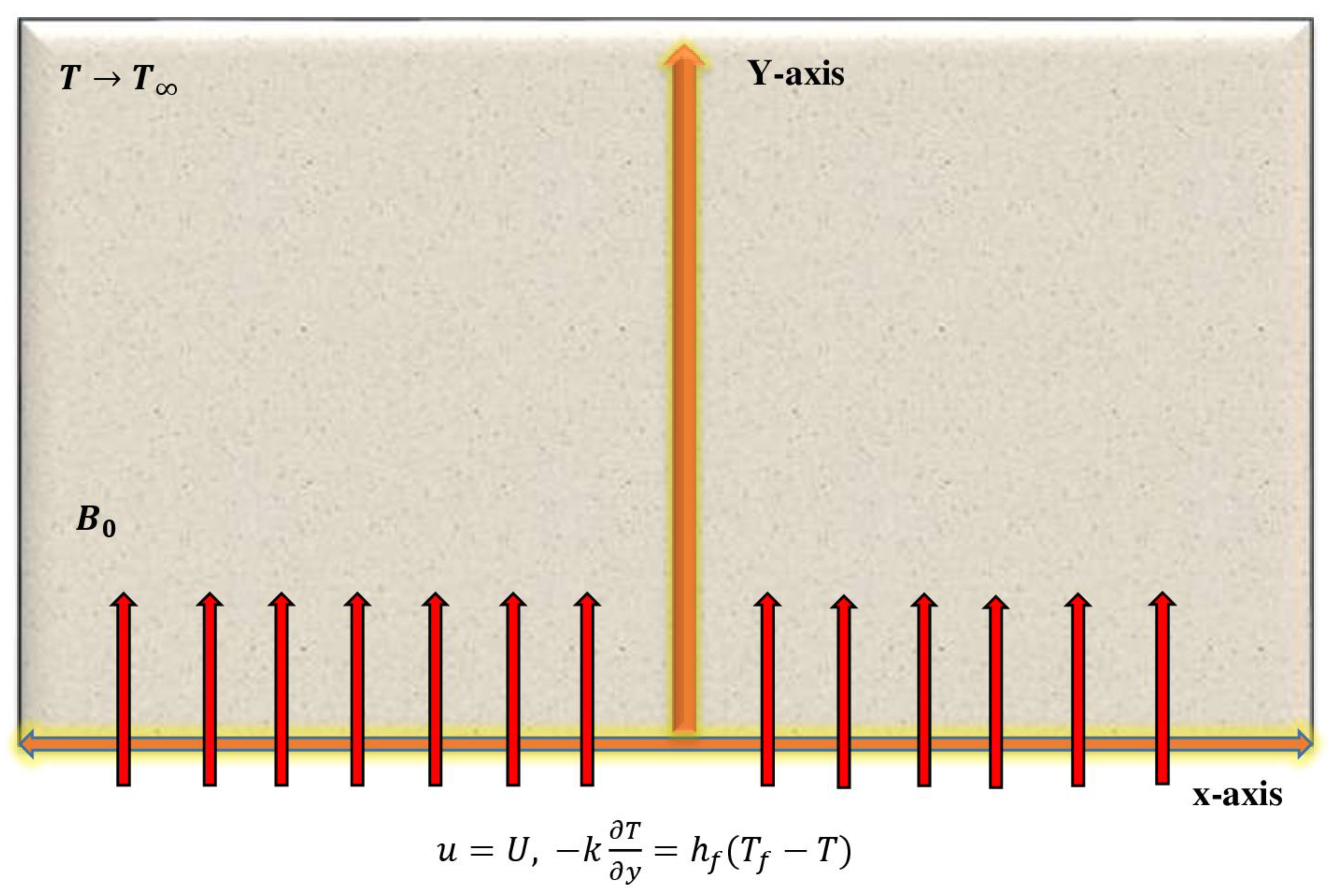
Consider the Oldroyd-B model rheology (a sort of fluid model that is based on rates) when it passes through a wall. Within a porous medium, the Sakiadis flow condition has been considered. To forecast magneto-hydrodynamics, a transverse magnetic field of intensity B₀ is supplied, as illustrated in Figure 1. The thermal characteristics at the wall and within the system have been studied using the convective heat process. The flow with internal heat generation/absorption qualities is governed by mathematical formulae.

$$\frac{\partial u}{\partial x}+\frac{\partial v}{\partial y}=0$$

(1)

$$\begin{array}{l}\rho \left(\frac{\partial u}{\partial t}+u\frac{\partial u}{\partial x}+v\frac{\partial u}{\partial y}\right)=-\frac{\partial p}{\partial x}+\mu \left(\frac{{\partial }^{2}u}{\partial x^2}+\frac{{\partial }^{2}u}{\partial y^2}\right)-\sigma B_0^{2}u\\ \rho \left(\frac{\partial v}{\partial t}+u\frac{\partial v}{\partial x}+v\frac{\partial v}{\partial y}\right)=-\frac{\partial p}{\partial y}+\mu \left(\frac{{\partial }^{2}v}{\partial x^2}+\frac{{\partial }^{2}v}{\partial y^2}\right)-\sigma B_0^{2}v\end{array}$$

(2)

$$\left(1+{\xi }_1\frac{DS}{Dt}\right)=\eta +\eta {\xi }_2\left(\frac{D{A}_1}{Dt}\right),$$

(3)

$$\frac{D{a}_i}{Dt}-\frac{\partial a_i}{\partial t}-u_r{a}_{i,r}+u_{i,r}{a}_r=0$$

(4)

$$\rho C_p\left(\frac{\partial \theta }{\partial t}+u\frac{\partial \theta }{\partial x}+v\frac{\partial \theta }{\partial y}\right)=k\left(\frac{{\partial }^2\theta }{\partial x^2}+\frac{{\partial }^2\theta }{\partial y^2}\right)+q_r$$

(5)

here, the u and v signify the velocity components, $\rho$ stands for the density of the fluid, $S$ is the stress tenser, A₁ denotes the Rivlin–Ericksen tenser, ${\xi }_1$ is the relaxation time effect, ${\xi }_2$ represents the retardation time effect, $\eta$ is the dynamic viscosity, and D/Dt is the covariant derivative.

From Equations (2)–(5) we have:

$$\begin{array}{l}u\frac{\partial u}{\partial x}+v\frac{\partial u}{\partial y}=-{\xi }_1\left(u^2\frac{{\partial }^{2}u}{\partial x^2}+v^2\frac{{\partial }^{2}u}{\partial x^2}+2uv\frac{\partial u}{\partial y\partial x}\right)-\left(\frac{\sigma B_0^{2}u}{\rho }+\frac{\nu }{k}\right)\left(u+{\xi }_{1}v\frac{\nu }{k}\right)\\ +\nu \left[\frac{{\partial }^{2}u}{\partial y^2}+{\xi }_2\left(u\frac{{\partial }^{2}u}{\partial y^2\partial x}+v\frac{{\partial }^{3}u}{\partial y^3}-\frac{\partial u}{\partial x}\frac{{\partial }^{2}u}{\partial y^2}-\frac{\partial u}{\partial y}\frac{{\partial }^{2}v}{\partial y^2}\right)\right]\end{array}$$

(6)

$$u\frac{\partial \theta }{\partial x}+v\frac{\partial \theta }{\partial y}={\alpha }_m\frac{{\partial }^2\theta }{\partial y^2}-\frac{1}{\rho C_p}\frac{\partial q_r}{\partial y}+\frac{Q_0}{\rho C_p}(\theta -{\theta }_{\infty })$$

(7)

The related BC are [22]

$$\begin{array}{ll}u=U_u,v=0,-k\frac{\partial \theta }{\partial y}=h_f({\theta }_f-\theta ),& \mathrm{at}y=0\\ u\to 0,v\to 0,\theta \to {\theta }_{\infty }& \mathrm{at}y\to \infty \end{array}$$

(8)

It is worth noting that for ${\xi }_2=0$, the Maxwell model can be obtained. Furthermore, in the case of ${\xi }_1={\xi }_2=0$, a Newtonian fluid model is obtained. In the above equation, $\sigma$ and $\theta$ indicate the fluid’s conductivity and heating rate, respectively. Moreover, $B_0,K,c_p,{\alpha }_n,\mathrm{and}{Q}_0$ are the magnetic field strength, material porosity, heat capacity constancy, thermal conductivity, and inner heat permeation/absoption parameter, respectively, whereas the radiation thermal transit amount qr is described as $q_r=-\left(4{\sigma }^3/3k\right)\frac{\partial {\theta }^4}{\partial y}.$3

Using the transformation listed below [3,4],

$$\eta ={\left(\frac{U_w}{vx}y\right)}^{1/2},u=U_w\varsigma \prime ,v=-1/2{\left(\frac{v{U}_w}{x}y\right)}^{1/2}\left(\varsigma -\eta {\varsigma }^{\prime }\right),T(\eta )=\frac{\theta -{\theta }_{\infty }}{{\theta }_f-{\theta }_{\infty }}$$

(9)

Hence, Equations (5)–(8) become

$$\begin{array}{l}{\varsigma }^{‴}+\left(\frac{1}{2}\right){\varsigma \varsigma }^{″}-\frac{D_1}{2}\left(2\varsigma \varsigma {}^{\prime }\varsigma {}^{″}+\eta \varsigma {\prime }^2\varsigma {}^{″}+{\varsigma }^2\varsigma {}^{″}\right)-M^2\left(\varsigma {}^{\prime }-D_1\left(\varsigma -\eta \varsigma {}^{\prime }\right){\varsigma }^{″}\right)\\ -K\varsigma {}^{\prime }+K{D}_1\left(\varsigma \varsigma {}^{″}-\eta \varsigma {}^{\prime }\varsigma {}^{″}\right)+D_2\left(2\left(\eta \varsigma {}^{\prime }\varsigma {}^{‴}+\eta \varsigma {}^{\prime }\varsigma {}^{⁗}-\varsigma {}^{\prime }\varsigma {}^{‴}\right)-\varsigma {\varsigma }^{iv}-\varsigma {}^{\prime }{\prime }^2\right)=0\end{array}$$

(10)

$$T{}^{″}+Pr\left(\frac{1}{2}\varsigma T{}^{\prime }+hsT\right)+\frac{4}{3}{R}_{d}T{}^{″}=0$$

(11)

$$\begin{array}{ll}\varsigma (\eta )=0,\varsigma {}^{\prime }(\eta )=1,T{}^{\prime }(\eta )=-{\Upsilon }_1(1-T(\eta )),& \mathrm{at}\eta =0\\ \varsigma {}^{\prime }(\eta )\to 0,T(\eta )\to 0& \mathrm{at}\eta =\infty \end{array}$$

(12)

In Equation (10), $D_1\mathrm{and}{D}_2$ are the Deborah numbers, $M$ is the magnetic field, and $K$ is the porosity parameter. In Equation (11), $Pr$ is the Prandtl number, $hs$ is the heat source parameter, and $R_d$ is the thermal radiation parameter, which is defined as:

$$\begin{array}{l}{D}_1=\frac{{\xi }_{1}U}{2x},D_2=\frac{{\xi }_{2}U}{2x},M^2=\frac{\sigma B_0^2}{\rho U},K=\frac{v}{kU},R_d=\frac{16\sigma {\theta }_{\infty }^3}{3k\prime k^{*}},\\ Pr=\frac{\nu }{{\alpha }_n},hs=\frac{Q_0}{\rho C_{p}U}.\end{array}$$

The physical quantity of interest is the thermal radiation, and the wall is given by

$$N_u=\frac{x{q}_x}{k({\theta }_{\varsigma }-{\theta }_{\infty })}$$

(13)

where

$$q_w=-k{\left(\frac{\partial \theta }{\partial y}\right)}_{y=0}+{\left(q_r\right)}_{y=0}$$

(14)

In dimensionless form, we have

$$N{u}_x/{\mathrm{Re}}^{1/2}=-\left(1+\frac{4}{3}{R}_d\right)T^{\prime }(0)$$

(15)

In Equations (14) and (15), $q_w$ and $R_e$ denote the wall heat flux and Reynolds number, respectively.

3. Numerical Procedure and Validation

The forward, backward, and central difference method was developed in order to obtain the numerical solution for the system of nonlinear higher order differential equations. For this goal, the ODEs are first converted to first order ODEs by using a suitable transformation along with boundary conditions. Then, they are solved by the RK-4 built-in function in MATLAB [38,39,40,41]. The Shooting technique is used to integrate a definite value for h. If the right step size Dh is chosen, this technique contains a procedure for calculating the solution. At each stage, two different solution estimations are generated and assessed. The assumption is approved if the two answers are close; otherwise, the step size is reduced until the desired precision is achieved. We utilised a Dh = 0.01 step size and accuracy to the fifth decimal point for this project. Figure 2 shows the flow chart for the numerical system.

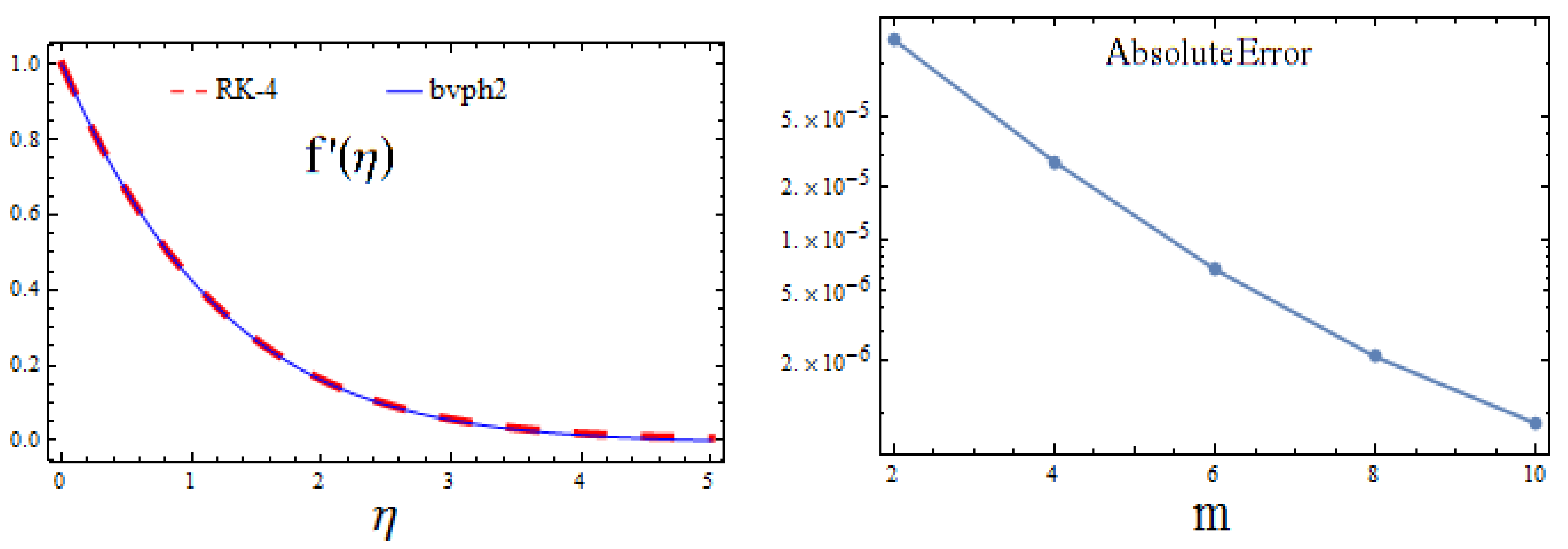
Equations (10) and (11) and boundary condition (12) are extremely nonlinear and interconnected. As a consequence, the error analysis was carried out in order to obtain the confirmed data. The code is also validated using Bvph2, and great agreement is found. The confirmation of two approaches, RK-4 and bvph2, as well as the CPU time up to the 10th iteration order, is shown in

Table 1. RK-4 and bvph2 evaluations for 20th order approximation with CPU time.

m	bvph2	RK-4	CPU Time (s)
2	3.1 × 10−6	1.3 × 10−4	1.179692
3	3.0 × 10−8	2.7 × 10−5	5.9045437
4	4.9 × 10−10	6.71 × 10−6	20.1231686
5	6.9 × 10−12	2.1 × 10−6	50.4153629
6	1.5 × 10−13	8.8 × 10−7	110.9415963
7	2.4 × 10−15	4.4 × 10−7	217.3541494
8	6.0 × 10−17	2.4 × 10−7	404.8458581
9	1.1 × 10−18	1.5 × 10−7	716.4912224
10	2.8 × 10−20	9.1 × 10−8	1213.6447644
20	5.3 × 10−22	5.7 × 10−8	2262.5860728

. As seen in this table, the computation error is rather small. Additionally, the residual error of RK-4 and bvph2 is also given in tabular form for the velocity and temperature profiles.

Table 2. Validation of RK-4 and bvph2 for the velocity field.

η	RK-4	bvph2	Absolute Error
0	1.000000	1.000000	1.110220 × 10−16
0.5	0.661166	0.660837	0.000330
1.0	0.425501	0.424831	0.000670
1.5	0.266090	0.265040	0.001050
2.0	0.162121	0.160630	0.001491
2.5	0.096694	0.094680	0.002014
3.0	0.056780	0.054141	0.002639
3.5	0.033032	0.029642	0.003390
4.0	0.019178	0.014881	0.004297
4.5	0.011226	0.005830	0.005396
5.0	0.006738	−1.046940 × 10−7	0.006738

shows the comparison of the RK-4 and bvph2, which clarifies that the precision is comparatively insignificant for the velocity profile. The current study is compared to the published work reported by Gireesha et al. [3] for additional confirmation, and good agreement is discovered, as shown in

Table 3. Validation of the present work and the published work reported by Gireesha et al. [22].

η	Present Work	Published Work [3]
0	1.000000	1.000000
0.5	0.661166	0.661163
1.0	0.425501	0.425502
1.5	0.266090	0.266094
2.0	0.162121	0.162120
2.5	0.096694	0.096693
3.0	0.056780	0.056781
3.5	0.033032	0.033034
4.0	0.019178	0.019175
4.5	0.011226	0.011223
5.0	0.006738	0.006739

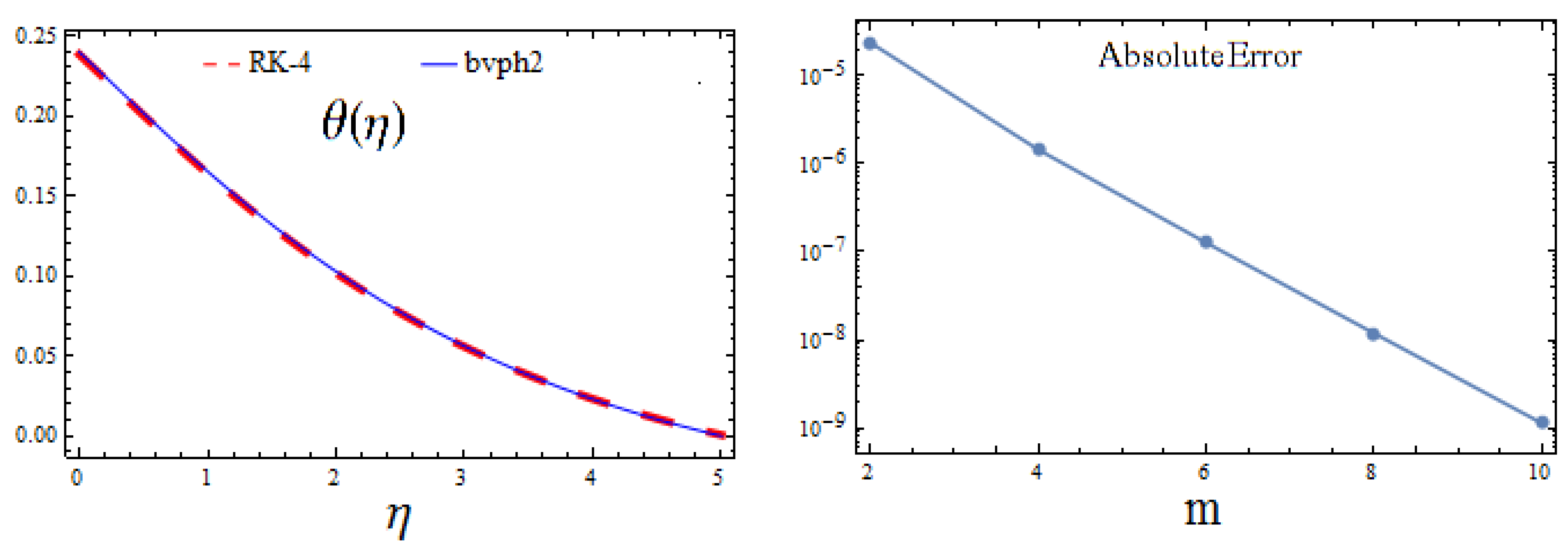
. Figure 3 and Figure 4 show the validity of these two approaches as well. Similarly, for the temperature profile, the validation of RK-4 and bvph2 is given in

Table 4. Validation of RK-4 and bvph2 for the temperature field.

η	RK-4	bvph2	Absolute Error
0	0.238311	0.239864	0.001553
0.5	0.200323	0.201763	0.001441
1.0	0.163895	0.165234	0.001339
1.5	0.130803	0.131982	0.001179
2.0	0.101765	0.102711	0.000947
2.5	0.076819	0.077492	0.000674
3.0	0.055675	0.056063	0.000388
3.5	0.037915	0.038021	0.000107
4.0	0.023095	0.022934	0.000160
4.5	0.010787	0.010385	0.000401
5.0	0.000613	3.023300×10-10	0.000613

.

4. Results and Discussion

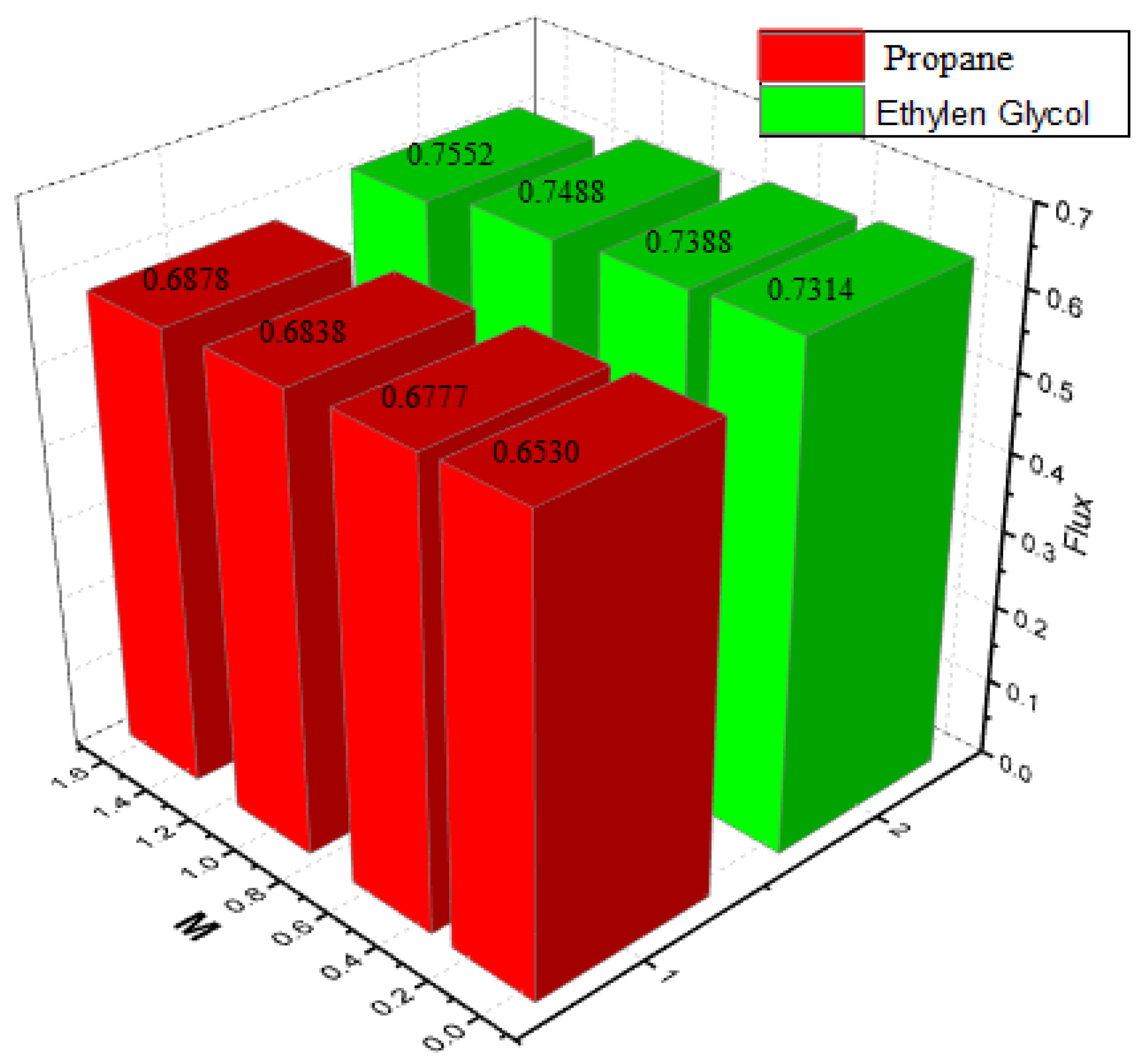
It should be emphasised that the wall convection parameter, internal generation or absorption quantity of heat, magnetic parameter, Deborah numbers, and other physical and rheological parameters are all included in the system of nonlinear equations (Equations (10)–(12)). As a result, we have created Figure 5, Figure 6, Figure 7, Figure 8, Figure 9, Figure 10, Figure 11 and Figure 12. For different magnetic parameter M values, the heat transfer rate is shown in Figure 5. The findings of propane are displayed in the front red bar, while the results of ethylene glycol are displayed in the green bar. When the magnetic is raised, the heat transfer rate drops in both cases. 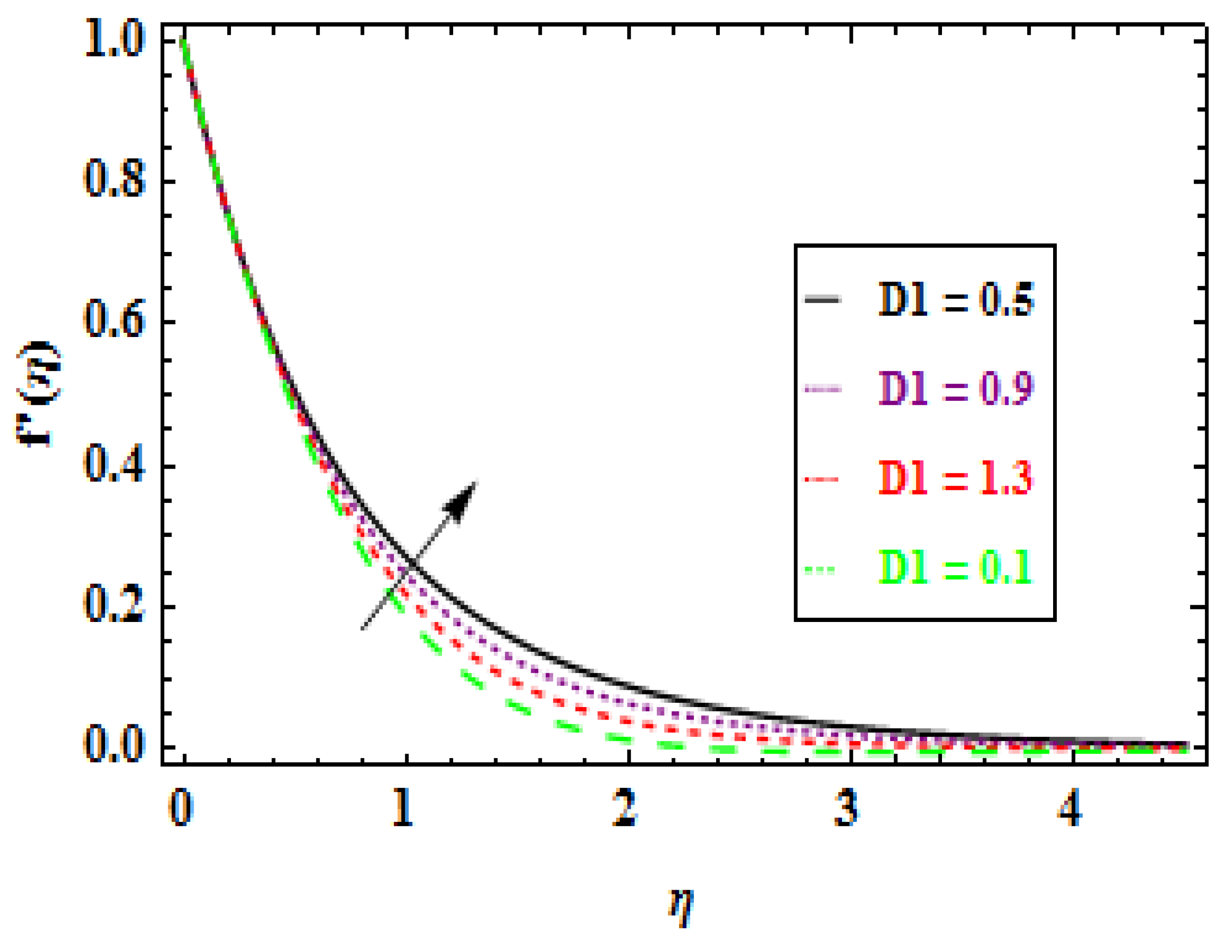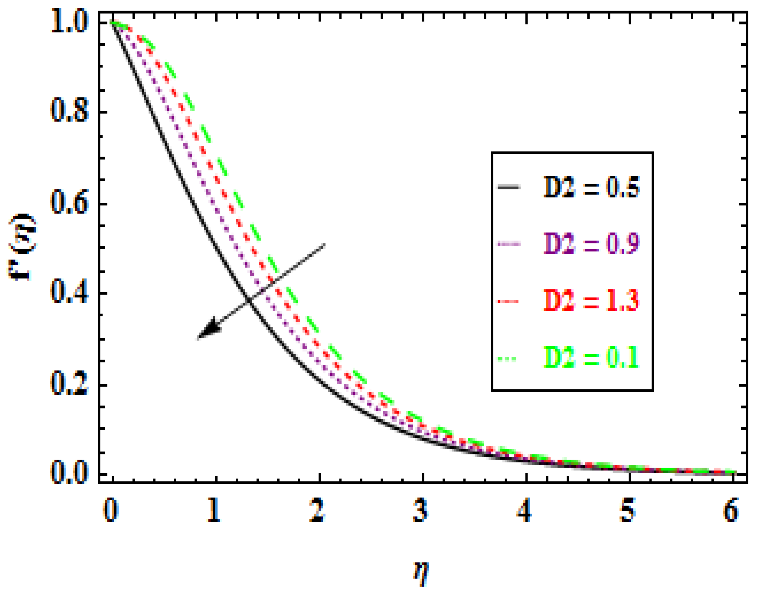The Deborah numbers (D₁ and D₂) influence the flow field, as illustrated in Figure 6 and Figure 7. As the Deborah number D₁ increases, the thickness of the boundary layer and the velocity profile both decrease, but as the Deborah number D₂ increases, the velocity profile declines. Deborah numbers with small values (D₁, D₂ << 1) represent flowing behaviour, whereas those with large values (D₁, D₂ >> 1) represent solid-like activity. Furthermore, the velocity profile shows an opposite trend for positive D₁ and D₂ values. 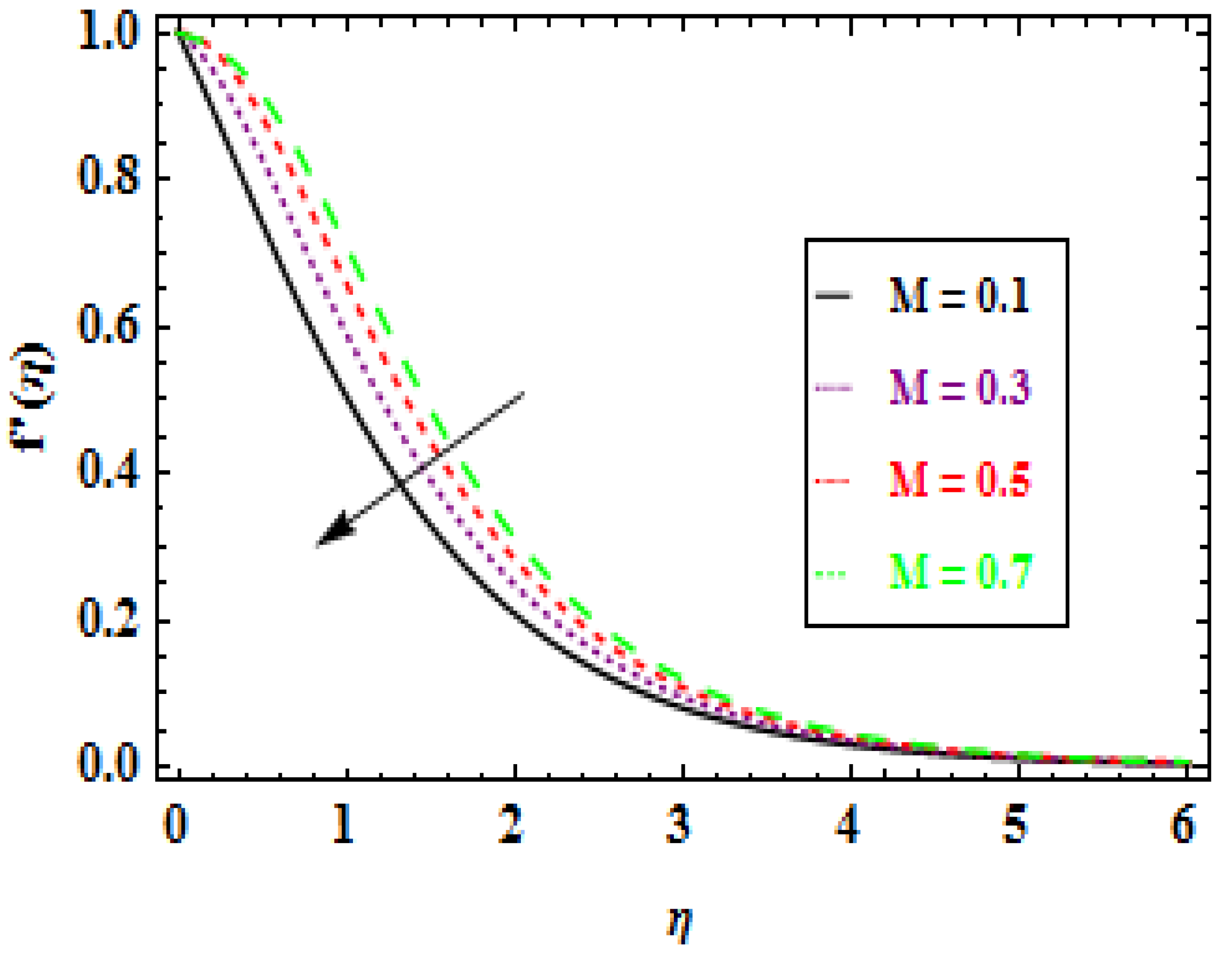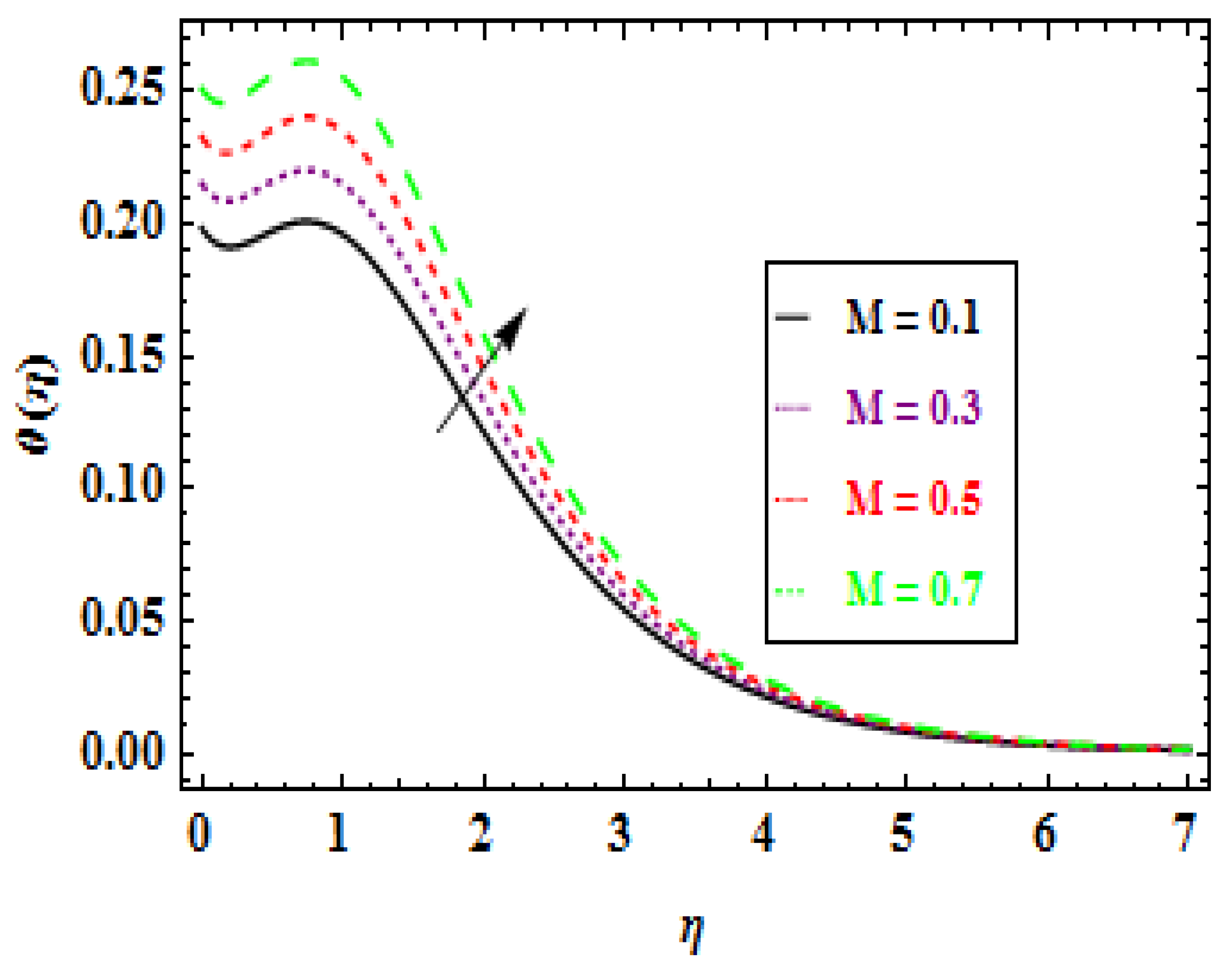Figure 8 illustrates the velocity profile’s dependence on the magnetic field M. The magnetic parameter and the fluid velocity have an inverse relationship, as we have seen. The temperature profiles of the magnetic parameter M for various magnitudes are shown in Figure 9. The temperature and thermal boundary layer thickness improves as the magnetic parameter M increases. It is clear that the velocity of fluid and the velocity boundary layer shrink with enhancing M for both fluids. This is due to the fact that the magnetic field is normal to the fluid’s direction, as the magnetic force in an opposite direction of the flow leads to an increase in the absorption of stationary fluid on the wedge and declines the speed of the flow. Therefore, the flow becomes heavier and needs further time to move. Moreover, the velocity boundary layer is thicker in the case of non-Newtonian fluid compared to Newtonian fluid. 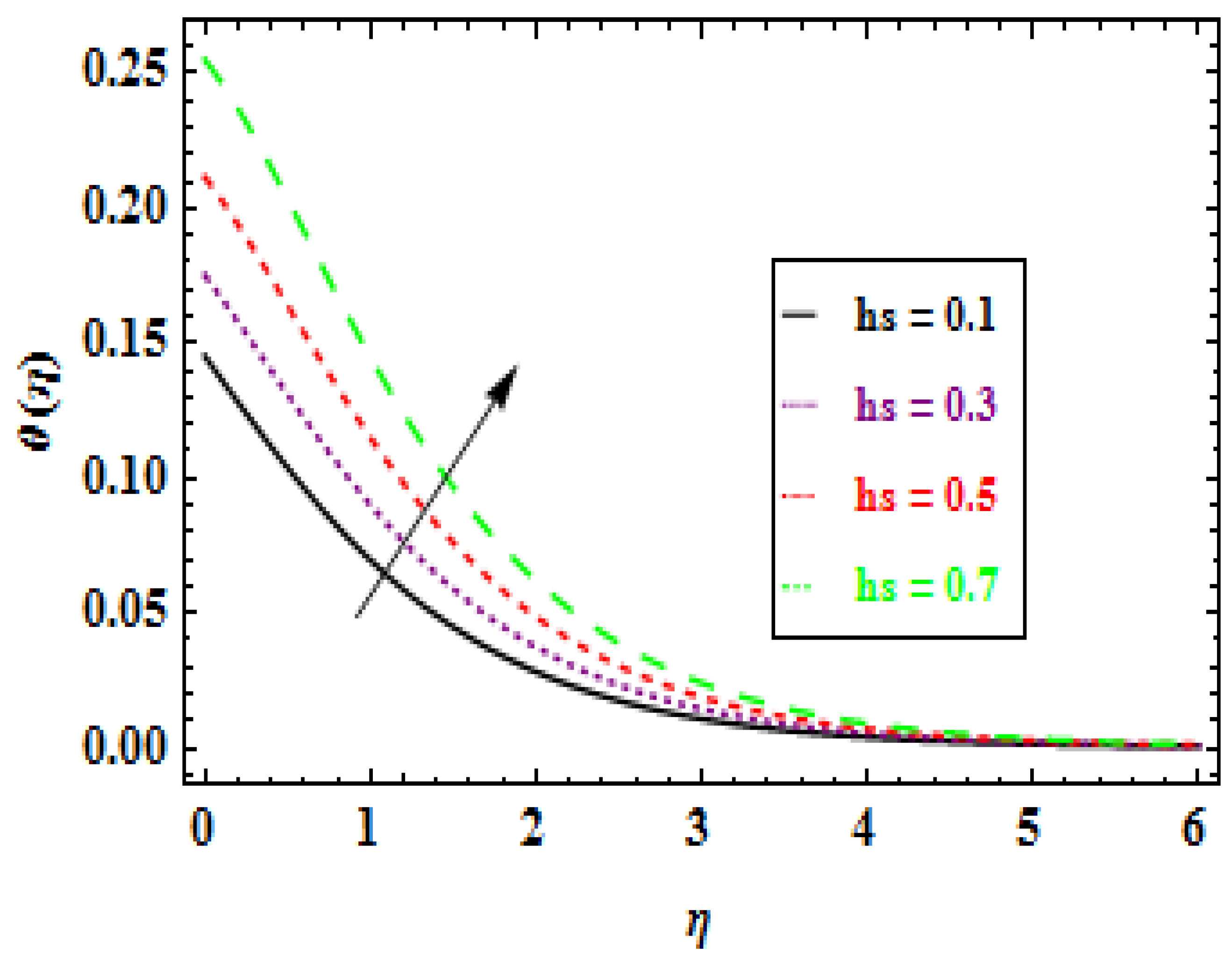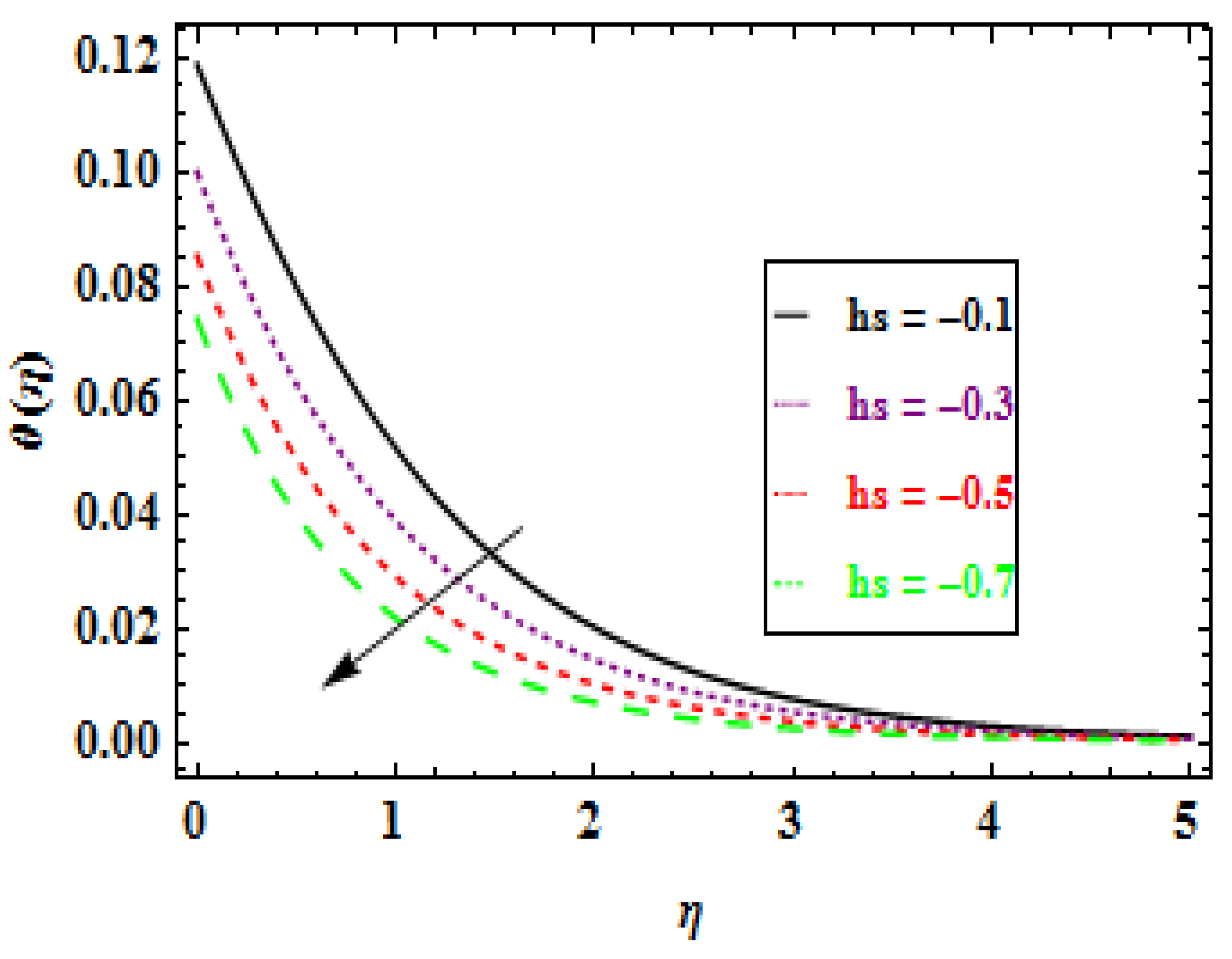The temperature profile is illustrated in Figure 10 with the internal heat absorption or generation parameter hs influence. Figure 10 and Figure 11 demonstrate the influence of the internal heat generation/absorption parameter hs on the temperature profile. Heat absorption is represented by hs < 0, whereas heat generation is represented by hs > 0. The temperature and its associated boundary layer appear to be dropping as a function of the heat absorption coefficient, whereas the temperature appears to be increasing in the case of heat generation. 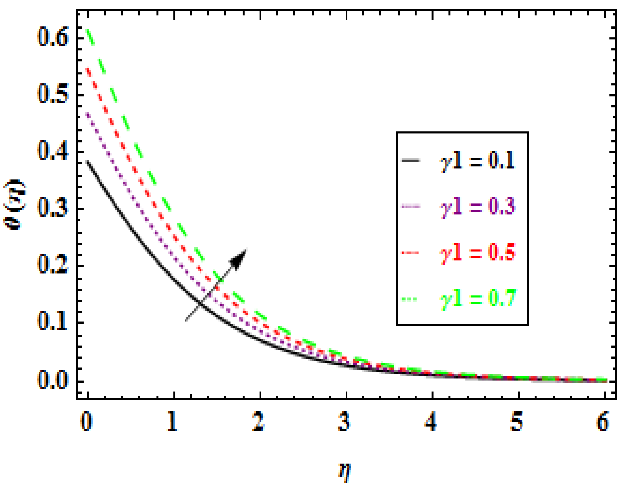Figure 12 depicts the temperature profile variation for various Biot number ${\gamma }_1$ values. For large values of ${\gamma }_1$, the temperature and thermal boundary layer thickness show a rising pattern. The most diversity may be seen near the moving wall, where the stream weakens gradually and tends to a uniform free stream.

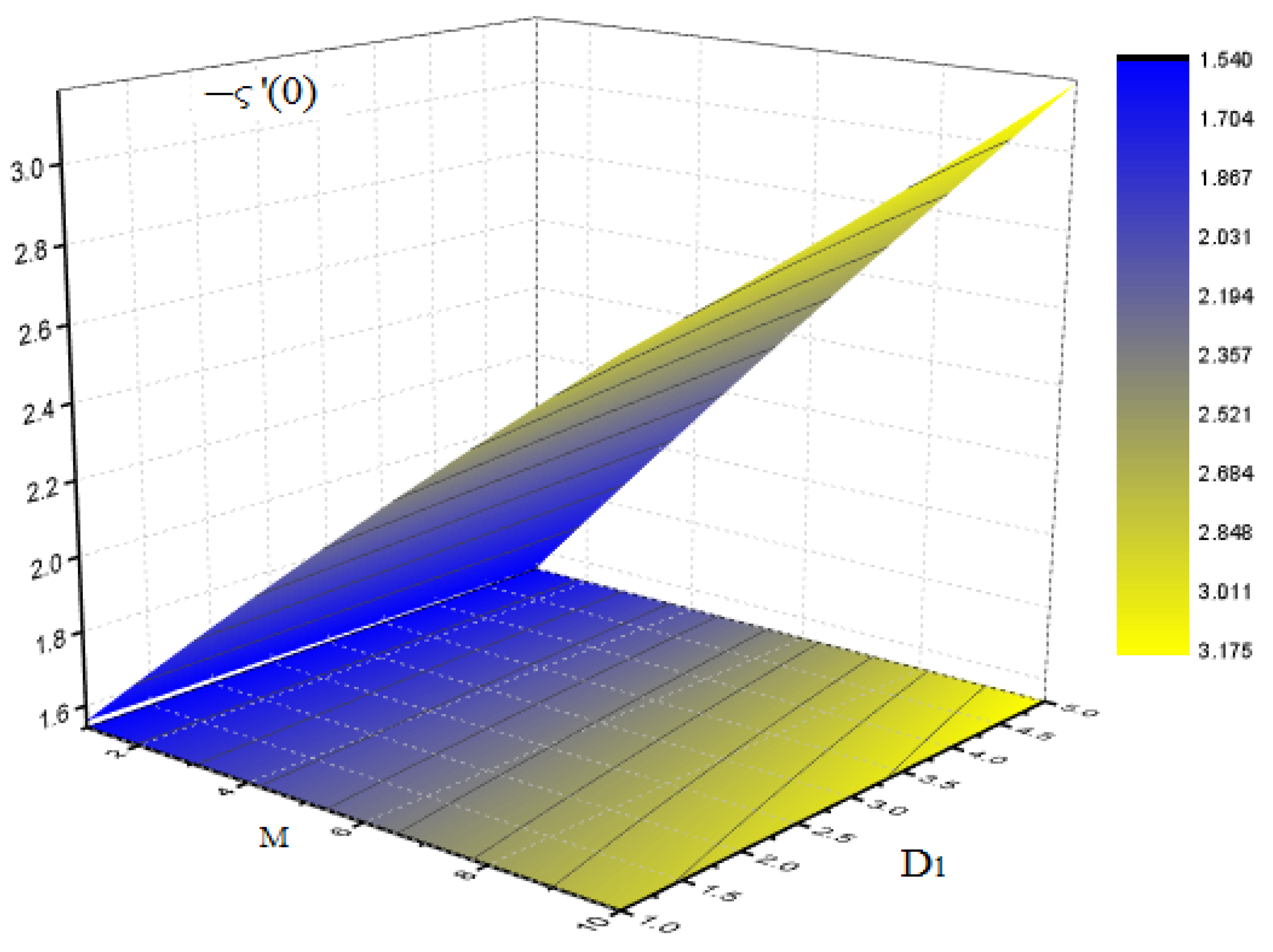
The quantitative magnitudes of local skin friction and local Nusselt numbers versus numerous rheological parameters are presented in Figure 13, Figure 14, Figure 15, Figure 16 and Figure 17 (3D graphs) and

Table 5. Influence of D₁ on −ς″(0).

Parameters							Numerical Solutions
D1	hs	M	D2	Pr	K	${\mathit{\gamma }}_1$	$-{\mathit{\varsigma }}^{″}(0)$
0.0	0.3	1	0.3	5.0	0.3	0.3	1.827825
0.3	0.3	1	0.3	5.0	0.3	0.3	1.884447
1.2	0.3	1	0.3	5.0	0.3	0.3	2.147765
1.6	0.3	1	0.3	5.0	0.3	0.3	2.215865

,

Table 6. Influence of hs on −ς″(0).

Parameters							Numerical Solutions
D1	hs	M	D2	Pr	K	γ1	−ς″(0)
0.3	−1.3	1	0.3	5.0	0.3	0.3	1.884447
0.3	−1	1	0.3	5.0	0.3	0.3	1.884447
0.3	−0.3	1	0.3	5.0	0.3	0.3	1.884458

,

Table 7. Influence of positive hs on −ς″(0).

Parameters							Numerical Solutions
D1	hs	M	D2	Pr	K	γ1	−ς″(0)
0.3	0	1	0.3	5.0	0.3	0.3	1.884431
0.3	0.4	1	0.3	5.0	0.3	0.3	1.884440
0.3	1.0	1	0.3	5.0	0.3	0.3	1.884440
0.3	1.3	1	0.3	5.0	0.3	0.3	1.885916

,

Table 8. Influence of M on −ς″(0).

Parameters							Numerical Solutions
D1	hs	M	D2	Pr	K	γ1	−ς″(0)
0.3	0.3	0	0.3	5.0	0.3	0.3	1.366983
0.3	0.3	0.2	0.3	5.0	0.3	0.3	1.571414
0.3	0.3	0.8	0.3	5.0	0.3	0.3	1.884441
0.3	0.3	1.5	0.3	5.0	0.3	0.3	2.458771

,

Table 9. Influence of D2 on −ς″(0).

Parameters							Numerical Solutions
D1	hs	M	D2	Pr	K	γ1	−ς″(0)
0.3	0.3	1	0	5.0	0.3	0.3	1.414718
0.3	0.3	1	0.4	5.0	0.3	0.	1.884432
0.3	0.3	1	1.1	5.0	0.3	0.3	4.277341
0.3	0.3	1	1.5	5.0	0.3	0.3	10.97555

,

Table 10. Influence of Pr on −ς″(0).

Parameters							Numerical Solutions
D1	hs	M	D2	Pr	K	γ1	−ς″(0)
0.3	0.3	1	0.3	2	0.3	0.3	1.884461
0.3	0.3	1	0.3	4	0.3	0.3	1.884461
0.3	0.3	1	0.3	6	0.3	0.3	1.884460
0.3	0.3	1	0.3	8	0.3	0.3	1.884460

,

Table 11. Influence of K on −ς″(0).

Parameters							Numerical Solutions
D1	hs	M	D2	Pr	K	γ1	−ς″(0)
0.3	0.3	1	0.3	5.0	0.0	0.3	1.763755
0.3	0.3	1	0.3	5.0	0.4	0.3	1.884419
0.3	0.3	1	0.3	5.0	1.2	0.3	2.358429
0.3	0.3	1	0.3	5.0	1.6	0.3	2.586296

,

Table 12. Influence of γ₁ on −ς″(0).

Parameters							Numerical Solutions
D1	hs	M	D2	Pr	K	γ1	−ς″(0)
0.3	0.3	1	0.3	5.0	0.3	0.2	1.884441
0.3	0.3	1	0.3	5.0	0.3	0.6	1.884441
0.3	0.3	1	0.3	5.0	0.3	1.2	1.884441

,

Table 13. Influence of D₁ on the wall temperature.

Parameters							Numerical Solutions
D1	hs	M	D2	Pr	K	${\mathit{\gamma }}_1$	$(1+\frac{4}{3}{\mathit{R}}_{\mathit{d}})\mathit{T}{}^{\prime }(0)$
0.0	0.5	1.0	0.5	1.0	0.5	0.5	0.88626087
0.5	0.5	1.0	0.5	1.0	0.5	0.5	0.87047844
1.0	0.5	1.0	0.5	1.0	0.5	0.5	0.85857029
1.5	0.5	1.0	0.5	1.0	0.5	0.5	0.84965734

,

Table 14. Influence of hs (negative) on the wall temperature.

Parameters							Numerical Solutions
D1	hs	M	D2	Pr	K	${\mathit{\gamma }}_1$	$(1+\frac{4}{3}{\mathit{R}}_{\mathit{d}})\mathit{T}{}^{\prime }(0)$
0.5	−1.5	1.0	0.5	1.0	0.5	0.5	0.47848456
0.5	−1	1.0	0.5	1.0	0.5	0.5	0.44917061
0.5	−0.5	1.0	0.5	1.0	0.5	0.5	0.39803006

,

Table 15. Influence of hs (positive) on the wall temperature.

Parameters							Numerical Solutions
D1	hs	M	D2	Pr	K	${\mathit{\gamma }}_1$	$(1+\frac{4}{3}{\mathit{R}}_{\mathit{d}})\mathit{T}{}^{\prime }(0)$
0.5	0	1.0	0.5	1.0	0.5	0.5	0.25191604
0.5	0.5	1.0	0.5	1.0	0.5	0.5	0.35714342
0.5	1.0	1.0	0.5	1.0	0.5	0.5	0.72566043
0.5	1.5	1.0	0.5	1.0	0.5	0.5	0.87047844

,

Table 16. Influence of M on the wall temperature.

Parameters							Numerical Solutions
D1	hs	M	D2	Pr	K	${\mathit{\gamma }}_1$	$(1+\frac{4}{3}{\mathit{R}}_{\mathit{d}})\mathit{T}{}^{\prime }(0)$
0.5	0.5	0.0	0.5	1.0	0.5	0.5	0.96221819
0.5	0.5	0.5	0.5	1.0	0.5	0.5	0.92237457
0.5	0.5	1.0	0.5	1.0	0.5	0.5	0.87047844
0.5	0.5	1.3	0.5	1.0	0.5	0.5	0.85099774

,

Table 17. Influence of D₂ on the wall temperature.

Parameters							Numerical Solutions
D1	hs	M	D2	Pr	K	${\mathit{\gamma }}_1$	$(1+\frac{4}{3}{\mathit{R}}_{\mathit{d}})\mathit{T}{}^{\prime }(0)$
0.5	0.5	1.0	0	1.0	0.5	0.5	−0.01897348
0.5	0.5	1.0	0.5	1.0	0.5	0.5	0.87047844
0.5	0.5	1.0	1.0	1.0	0.5	0.5	0.84028696
0.5	0.5	1.0	1.5	1.0	0.5	0.5	0.82674776

,

Table 18. Influence of Pr on the wall temperature.

Parameters							Numerical Solutions
D1	hs	M	D2	Pr	K	${\mathit{\gamma }}_1$	$(1+\frac{4}{3}{\mathit{R}}_{\mathit{d}})\mathit{T}{}^{\prime }(0)$
0.5	0.5	1.0	0.5	0.1	0.5	0.5	0.15693718
0.5	0.5	1.0	0.5	0.5	0.5	0.5	−0.44869951
0.5	0.5	1.0	0.5	1.0	0.5	0.5	0.87047844
0.5	0.5	1.0	0.5	1.5	0.5	0.5	0.52974335

,

Table 19. Influence of K on the wall temperature.

Parameters							Numerical Solutions
D1	hs	M	D2	Pr	K	${\mathit{\gamma }}_1$	$(1+\frac{4}{3}{\mathit{R}}_{\mathit{d}})\mathit{T}{}^{\prime }(0)$
0.5	0.5	1.0	0.5	1.0	0.0	0.5	0.21824554
0.5	0.5	1.0	0.5	1.0	0.5	0.5	0.87047844
0.5	0.5	1.0	0.5	1.0	1.0	0.5	0.85515317
0.5	0.5	1.0	0.5	1.0	1.5	0.5	0.84547170

,

Table 20. Influence of γ₁ on the wall temperature.

Parameters							Numerical Solutions
D1	hs	M	D2	Pr	K	${\mathit{\gamma }}_1$	$(1+\frac{4}{3}{\mathit{R}}_{\mathit{d}})\mathit{T}’(0)$
0.5	0.5	1.0	0.5	1.0	0.5	0.1	0.14570719
0.5	0.5	1.0	0.5	1.0	0.5	0.5	0.87047844
0.5	0.5	1.0	0.5	1.0	0.5	1.0	2.30145457
0.5	0.5	1.0	0.5	1.0	0.5	1.5	5.09132362

and

Table 21. Comparison of non-Newtonain and Newtonian (ξ₁ = ξ₂ = 0) fluids.

η	Non-Newtonian	Newtonian
0	1.000000	1.000000
0.5	0.661166	0.661167
1.0	0.425501	0.425512
1.5	0.266090	0.266005
2.0	0.162121	0.162100
2.5	0.096694	0.096687
3.0	0.056780	0.056780
3.5	0.033032	0.033034
4.0	0.019178	0.019179
4.5	0.011226	0.011230
5.0	0.006738	0.006740

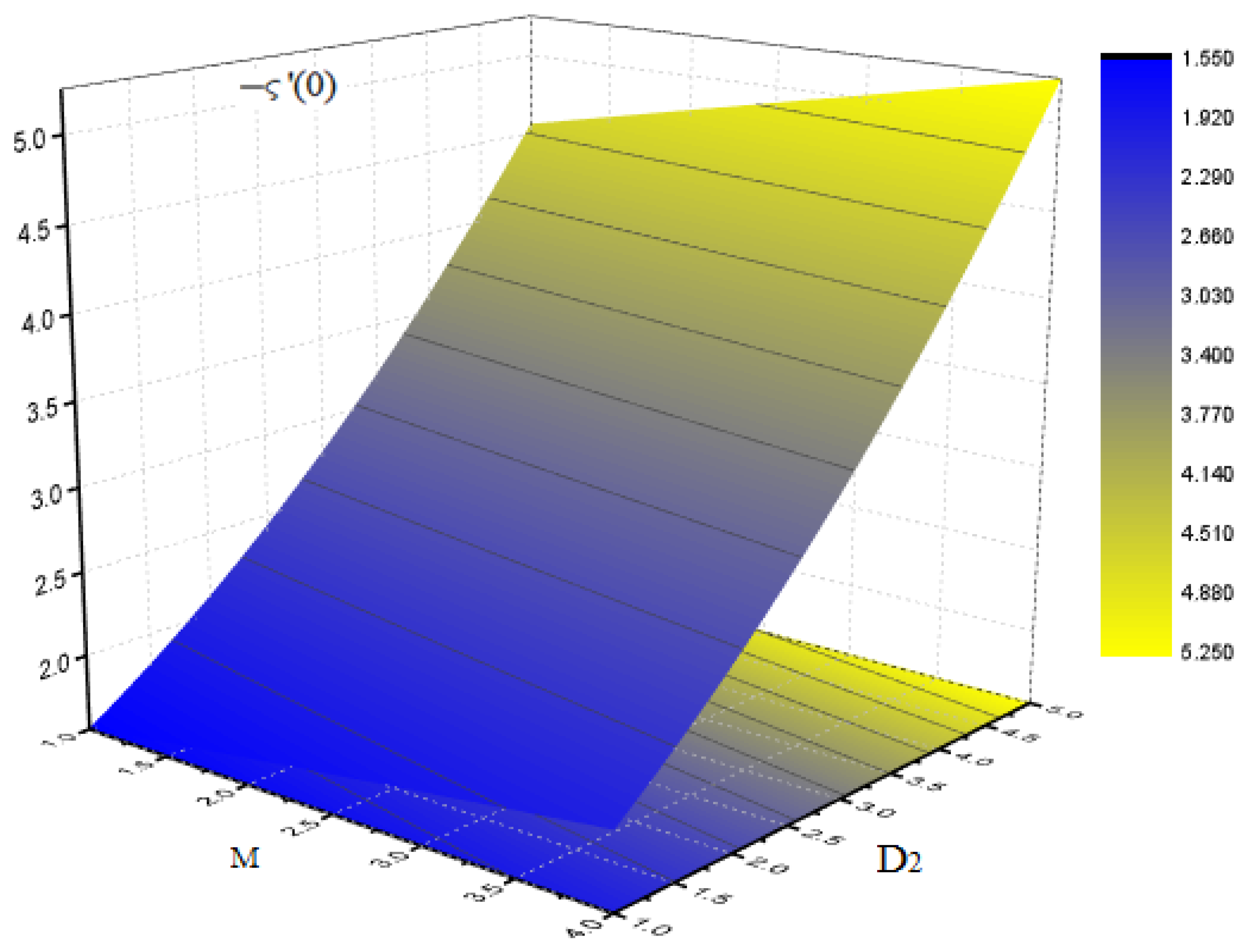
. Figure 13 represents the influence of D₁ and M on the local skin friction. From this study, it is analysed that the skin friction enhances as the D₁ and M are enhanced. This is due to the Lorentz force, which resists the flow and increases the local skin friction. For various values of D₂ = 0.1, 0.4, 1.1, and 1.5, the variation in $-\varsigma {}^{″}(0)$ is investigated, as shown in Figure 14. It is perceived that the skin friction rises with the increasing values of D₂. Similarly, investigation has been observed in Figure 15.

Table 5, Table 6 and Table 7 represent the variation of D₁, hs (for positive and negative), and M on the local skin friction. The influence of the Deborah number D₁ on the skin friction is depicted in Table 5. From this analysis, it is observed that the skin friction increases as the D₁ enhances. Table 6 and Table 7 show that hs (hs > 0 (heat generation) and hs < 0 (heat absorption)) has no significant effect on the$-\varsigma {}^{″}(0)$. It is observed that $-\varsigma {}^{″}(0)$ enhances as the magnetic parameter increases. This is due to the Lorentz force, which resists the flow and increases the local skin friction, as shown in Table 8. 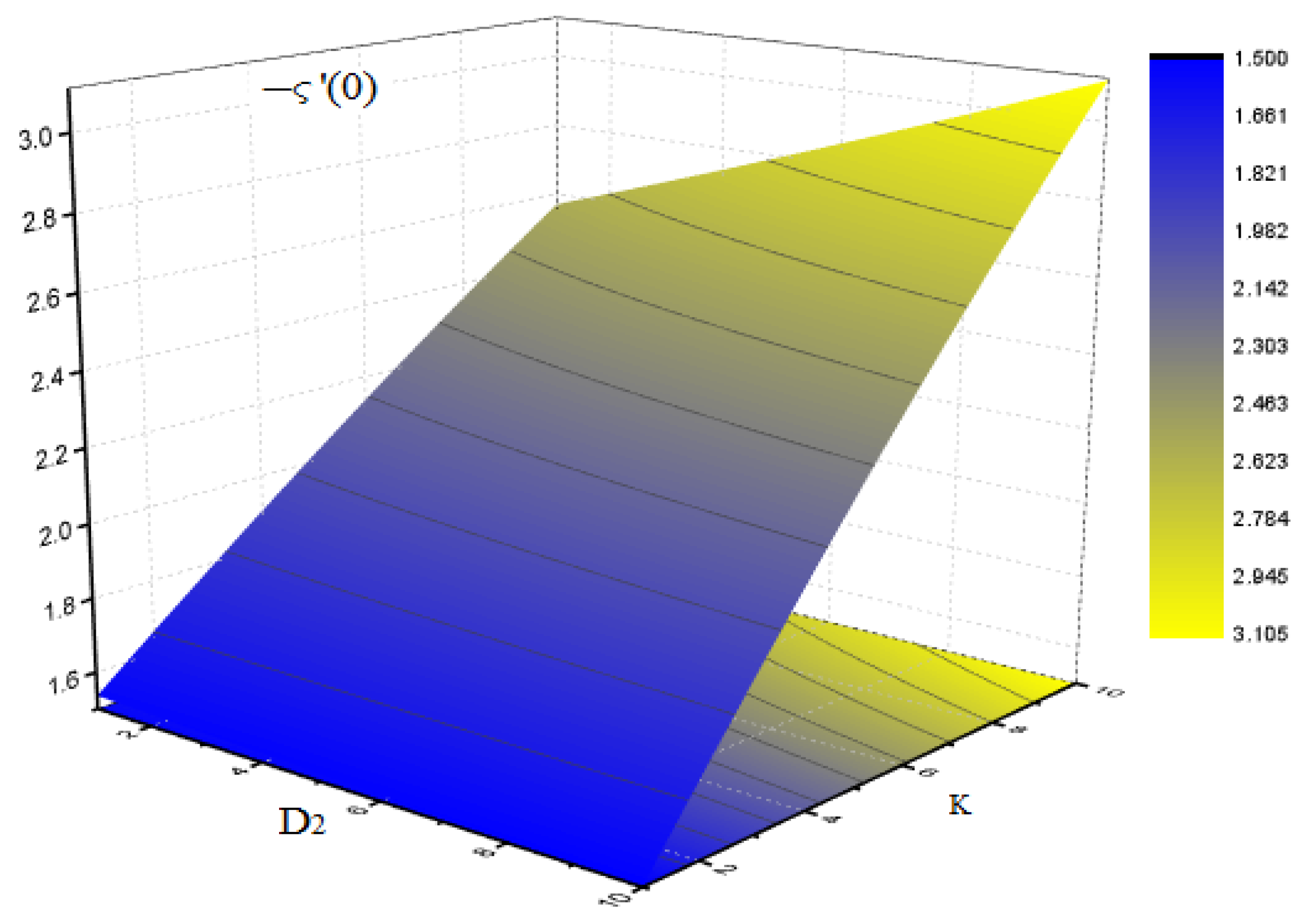Table 9, Table 10, Table 11 and Table 12 show the influence of the physical parameters D₂, Pr, K, and ${\gamma }_1$ on the skin friction. For various values of D₂ = 0.1, 0.4, 1.1, and 1.5, the variation in $-\varsigma {}^{″}(0)$ is investigated. It is perceived that the skin friction rises with the increasing values of D₂, as shown in Table 9. The ratio of momentum diffusivity to heat diffusivity is described by Pr, a dimensionless quantity. This number contrasts the effects of the viscosity and heat conductivity of a fluid. The sort of fluid we are looking at is determined by the Pr number. High thermal conductivity and low Pr values characterise the heat-transmitting fluids. As seen in Table 10, raising the Pr number has little impact on skin friction and has no discernible effect. Similarly, raising the value of K in Table 11 enhances the impact. The non-dimensional heat generation/absorption parameter ${\gamma }_1$ relies on the quantity of heat created by or absorbed in the fluid, and its impact on the skin friction is comparable to that of Pr, as shown in Table 12.

Table 13, Table 14, Table 15, Table 16, Table 17, Table 18, Table 19 and Table 20 display the variation of the Nusselt number for numerous values of the physical parameters D₁, hs (both positive and negative), M, D₂, Pr, K, and ${\gamma }_1$. Table 13 depicts the effect of D₁ on the Nusselt number. It is detected that the Nusselt number enhances as D₁ is increased. The variation of hs (hs > 0 (heat generation), hs < 0 (heat absorption)) on the Nusselt number is indicated in Table 14 and Table 15. It is predicted that the Nusselt number increases for hs > 0 and declines for hs < 0, respectively. The demonstration of the Nusselt number for the physical parameters M, D₂, Pr, and ${\gamma }_1$ on the Nusselt number is shown in Table 16, Table 17, Table 18, Table 19 and Table 20. It is perceived that the Nusselt number drops for the increasing values of the physical parameters M, D₂, and Pr. The ratio of momentum diffusivity to heat diffusivity is introduced by this dimensionless variable. This number contrasts the effects of the viscosity and heat conductivity of a fluid. The Pr number indicates the type of fluid being evaluated. High thermal conductivity and low Pr values characterise heat-transmitting fluids. As seen in Table 18, the Prandtl number has little effect on the skin friction but boosts the Nusselt number. Likewise, the porosity has an increasing impact and the Biot number has a decreasing influence on the Nusselt number, as shown in Table 19 and Table 20, respectively. Additionally, a comparison of the Newtonian and non-Newtonian fluid for various values of the magnetic parameter M is given in Table 21 in the revised manuscript.

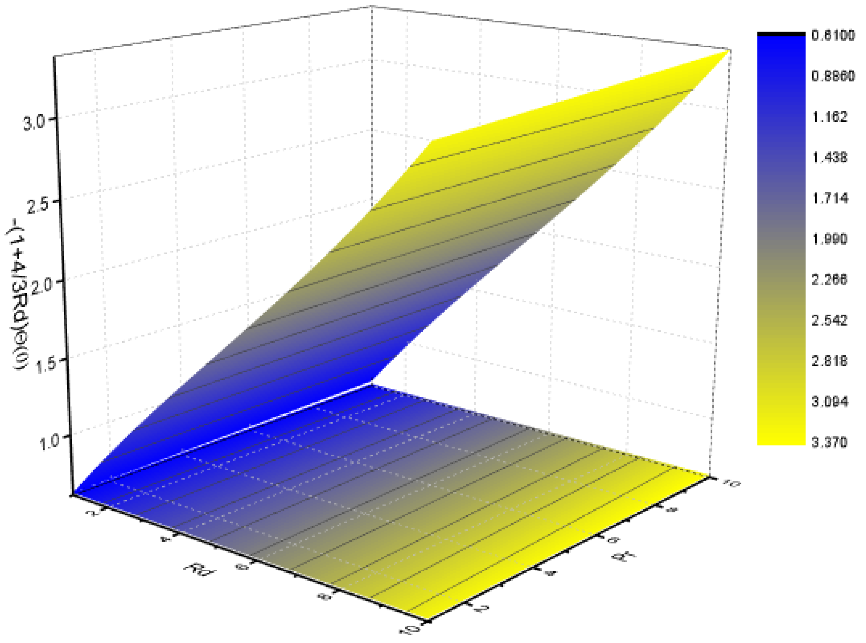
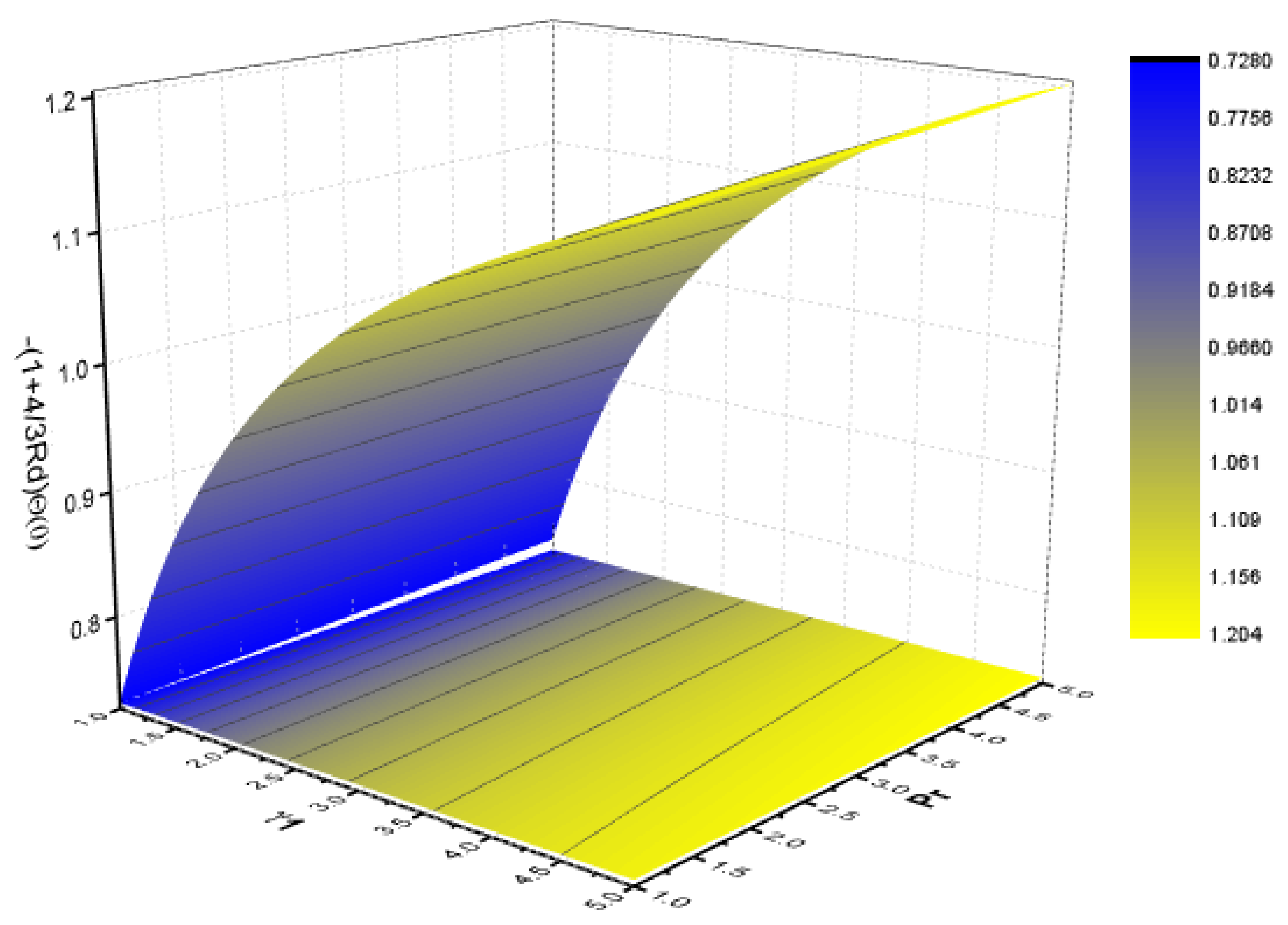
The combined effects of the physical parameters D₁, D₂, K, and M on the skin friction are presented Figure 13, Figure 14 and Figure 15. The parameters have a good influence on the skin friction. The influence of the Physical Parameters Pr, R_d, and ${\gamma }_1$ on the Nusselt number is presented in Figure 16 and Figure 17. These influences are already discussed separately in the above figures.

5. Conclusions

In this study, the fluid flows across a permeable wall with Sakiadis Oldroyd-B dynamics were investigated. The following are some of the study’s final outcomes, which are based on the graphical results:

• The velocity and momentum boundary layers diminish as the Deborah number D₁ increases, but both improve as the Deborah number D₂ increases.
• The Lorentz force, which resists the flow, reduces the velocity of the fluid as the magnetic parameter increases.
• By strengthening the magnetic field, the temperature profile rises.
• Over the temperature profile, opposite behaviours of heat generation and absorption effects are found.
• The temperature rises when the Biot number is high.
• From this analysis, it is observed that the skin friction increases as the D₁ enhances.
• It is observed that −Ϛ′′(0) enhances as the magnetic parameter increases. This is due to the Lorentz force, which resists the flow and increases the local skin friction.
• Heat conducting fluids have significant thermal conductivity and a low Prandtl number, but raising the Pr has little effect on the skin friction.
• It is predicted that the Nusselt number increases for hs > 0 and declines for hs < 0, respectively.
• In the future, exploring the potential stochastic numerical computing approaches using the procedures of Artificial Intelligence to analyse the Sakiadis flow dynamics of Oldroyd-B fluid via a porous wall model is intriguing.