
DEA and Machine Learning for Performance Prediction


International Business School, Beijing Foreign Studies University, Beijing 100089, China
*
Author to whom correspondence should be addressed.
Mathematics 2022, 10(10), 1776; https://0-doi-org.brum.beds.ac.uk/10.3390/math10101776
Submission received: 18 April 2022
/
Revised: 18 May 2022
/
Accepted: 22 May 2022
/
Published: 23 May 2022
(This article belongs to the Special Issue Quantitative Analysis and DEA Modeling in Applied Economics)
Abstract
:Data envelopment analysis (DEA) has been widely applied to evaluate the performance of banks, enterprises, governments, research institutions, hospitals, and other fields as a non-parametric estimation method for evaluating the relative effectiveness of research objects. However, the composition of its effective frontier surface is based on the input-output data of existing decision units, which makes it challenging to apply the method to predict the future performance level of other decision units. In this paper, the Slack Based Measure (SBM) model in DEA method is used to measure the relative efficiency values of decision units, and then, eleven machine learning models are used to train the absolute efficient frontier to be applied to the performance prediction of new decisions units. To further improve the prediction effect of the models, this paper proposes a training set under the DEA classification method, starting from the training-set sample selection and input feature indicators. In this paper, regression prediction of test set performance based on the training set under different classification combinations is performed, and the prediction effects of proportional relative indicators and absolute number indicators as machine-learning input features are explored. The robustness of the effective frontier surface under the integrated model is verified. An integrated models of DEA and machine learning with better prediction effects is proposed, taking China’s regional carbon-dioxide emission (carbon emission) performance prediction as an example. The novelty of this work is mainly as follows: firstly, the integrated model can achieve performance prediction by constructing an effective frontier surface, and the empirical results show that this is a feasible methodological technique. Secondly, two schemes to improve the prediction effectiveness of integrated models are discussed in terms of training set partitioning and feature selection, and the effectiveness of the schemes is demonstrated by using carbon-emission performance prediction as an example. This study has some application value and is a complement to the existing literature.
MSC:
90B501. Introduction
As a non-parametric analysis method, DEA extends the concept of single input and single output engineering efficiency to the efficiency evaluation of multi-input and multi-output decision units. This method was first proposed by Charnes, Cooper, and Rhodes in the United States in 1978 [1]. Due to its wide applicability, simple principle, and unique advantages especially in analyzing multiple inputs and outputs, it has been widely applied to the evaluation of performance of various organizations and regions in the past period. For example, bank operation performance evaluation [2,3,4,5,6], company operation performance evaluation [7,8,9,10] and regional carbon-emission performance evaluation [11,12,13,14,15,16,17]. However, the method has some limitations. First, based on the input and output data of the existing decision units, the effective frontier surface is determined, and the decision units on this effective frontier surface are all efficient. In addition, the efficiency value of each decision unit based on the distance of each unit to the effective frontier surface is determined. The effective frontier surface will be changed when new units are added. Moreover, the performance evaluation of the new year’s decision unit needs to be based on the new year’s effective frontier. If other decision units’ input and output data are not available, the effective frontier cannot be constructed for performance evaluation. In addition, the effective frontier of DEA is easily affected by statistical noise, which leads to frontier bias [18]. Finally, the DEA method cannot realize the prediction of new decision units.
The absolute efficient frontier can be constructed for solving above limitations of DEA by introducing machine learning methods. The efficiency values of new decision units can be found without re-measuring the whole decision units when new decision units are added. At the same time, it can predict the efficiency value of the new decision unit in the same period and the future efficiency value of the decision unit by regression. Finally, the presence of statistical noise can be overcome by repetitive training during the training with the machine learning models. Based on the integrated model of DEA and machine learning, to further improve the prediction effect of the integrated model, the following ideas are proposed in this paper in terms of training-set sample selection and composition of input feature indicators.
In terms of training-set sample selection, the DEA classification method is proposed in this paper when considering how to make the training set contain as much important feature information as possible. Based on the quartile method to classify the efficiency values of the measures into intervals, different combination strategies are proposed to verify which has more value, the more effective sample data or the relatively ineffective sample data. In this paper, an empirical study is conducted on the example of regional carbon-emission performance prediction in China.
In terms of the composition of input characteristic indicators, many current DEA application studies use proportional relative indicators to construct the input-output evaluation index system [19,20,21,22,23]. Theoretically, the production possibility set is a linear combination of decision units. The DEA method is a linear programming method based on this possibility set. The input and output indicators should be linearly additive. Otherwise, they may produce the wrong production possibility set and thus obtain unreliable results [24]. More intuitively, if the output indicator is a proportional (rate) indicator, the DEA model may measure an improvement target value greater than 100%, which is an illogical result. Therefore, this paper does not focus on whether the proportional indicators are reasonable in DEA, so we will not explore this issue. The use of proportional relative indicators as input-output indicators in DEA is somewhat controversial. However, proportional relative indicators are available as input feature variables in machine learning. The output characteristic variable of the machine learning model is the efficiency value of DEA measure, i.e., the ratio of weighted output to weighted input. If the proportional relative indicator is used as the input feature variable, its prediction effect may be better than using the absolute figure indicator. Based on this assumption, the empirical evidence will be developed later.
In summary, the contributions of this paper are mainly: (1) the use of an integrated model based on a non-radial SBM model and eleven machine learning methods, which is an extension of the existing methodological research. The SBM model uses a non-radial approach to introduce the relaxation variables directly into the objective function. Such an approach considers the full range of relaxation variables and allows for a more accurate assessment of efficiency values than the radial DEA model. Eleven machine learning models cover traditional and tree-based, and integrated machine learning models. (2) A DEA classification is proposed for training subset partitioning, composing different combinations of classifications for model training, and a comparative study on their specific prediction results is conducted. (3) A comparative study of the prediction effects of models with proportional relative indicators and absolute number indicators as machine-learning input features is conducted. (4) The efficiency measure under the new integrated model can be based on the absolute frontier surface, which can realize the measure of new decision units at the same time, on the one hand, or complete the measure of new decision units in future years. (5) The study of this performance prediction model increases the ideas and methods in carbon-emission performance prediction.
This paper is structured as follows. The second part introduces related studies. In the third part, an introduction to the basic models and methods involved in this study is given. In the fourth part, an empirical study and analysis are conducted on the example of regional carbon-emission performance prediction in China. The fifth part contains the results and discussion. Finally, the paper concludes with an outlook on future research directions.
2. Related Studies
By combing the literature of DEA methods and machine-learning integration methods, we can notice that some scholars have explored the situation of combining DEA with neural networks. Table 1 summarizes previous studies. Athanassopoulos and Curram [25] were the first to try to introduce neural networks into DEA, which was the first exploration in this area. The paper pointed out that DEA and neural networks, as non-parametric models, have some similar characteristics, which to some extent justifies the combination of DEA and neural networks. Wang [26] demonstrated that DEA can hardly be used to predict the performance of new decision units, and one good approach is to combine DEA and artificial neural networks (ANNs) which can help decision makers to construct a stable efficient frontier. Santin et al. [27] reviewed the application of ANNs to efficiency analysis, comparing efficiency techniques in nonlinear production functions comparison. They demonstrated that ANNs and DEA methods are non-parametric methods with some similarities, providing a basis for the subsequent combination of the two. A study by Wu et al. [28] pointed out that DEA has difficulties in predicting the performance of other decision units, and that problems in practice may exhibit great non-linearity. For example, the performance between financial indicators and efficiency is often nonlinear in bank efficiency analysis based on the performance characteristics of financial indicators. The nonlinearity can be better handled by introducing a neural network approach. They apply the combination of DEA and ANNs to the performance evaluation of Canadian banks. The empirical study showed that the method facilitates the construction of a more robust frontier surface and addresses the shortcomings of a purely linear DEA approach. Azadeh et al. [29] found that combining DEA and ANNs is a good complement to help in predicting efficiency. Emrouznejad and Shale [30] applied DEA and neural network methods to measure efficiency of large-scale datasets and demonstrated through empirical results that the integrated model can be a useful tool for measuring the efficiency of large datasets. Samoilenko and Osei-Bryson [31] proposed that neural networks should be able to assist DEA. Subsequently, a few scholars have explored somewhat in the field of integrated models of DEA and neural networks [32,33,34,35,36,37,38].
It can be seen that some relevant papers [25,26,27,28,29,30,31,32,33,34,35,36,37,38] have focused on the theoretical basis of the integrated model composed of DEA and neural network and applied it to some performance prediction problems. They have achieved good results through empirical studies and verified the reasonableness and feasibility of the integrated model of DEA and neural network. This provides valuable experience for further in-depth exploration. In any case, the current results still have the following problems and research gaps.
- They mostly use only DEA and a single neural network approach, especially ANNs in neural networks. Exploration of the combination of other machine learning methods is lacking.
- The existing literature studies mainly use the CCR and BCC models in DEA methods. These two models use the radial distance function. So, these two models for the measurement of the degree of inefficiency only include the part of all inputs (outputs) equal proportional changes, and do not take into account the part of slack improvement. Therefore, there are some shortcomings in the efficiency evaluation.
- After constructing the integrated model, related studies did not further explore how to improve performance prediction in terms of dataset composition and feature index selection.
3. Description of the Methodology
3.1. Data Envelopment Analysis (DEA)
Data Envelopment Analysis (DEA) is a tool instrument used to evaluate the relative effectiveness of work performance in the same type of organization. The principle of the method is to determine the relative effectiveness of the production frontier by keeping the inputs or outputs of the decision units constant with the help of mathematical planning and statistical data. The model projects each decision unit onto the DEA production frontier and evaluates their relative effectiveness by comparing how the decision units deviate from the DEA effective frontier.
3.1.1. DEA Base Model
In 1978, Charnes, Cooper, and Rhodes [1] proposed the first DEA model, the CCR model, which consists of the initials of three people’s last names. They extended the concept of single-input, single-output engineering efficiency to multiple-input and multiple-output relative efficiency evaluation. The CCR model has now become a familiar and essential tool for performance evaluation, taking input orientation as an example, with a specific planning equation as in Equation (1).
In the formula, the full name of “s.t.” is “subject to”, and it is usually followed by a number of constraints. Each decision unit has m kinds of input, denoted as , and the weight of the input is expressed as ; each decision unit has q kinds of output, denoted as , and the weight of the output is expressed as . The efficiency values obtained using the above weights for all decision units do not exceed 1. The detailed explanation of all parameters in all formulas is shown in Table A6 of Appendix A.
This equation is nonlinear and it has an infinity of optimal solutions, it becomes a problem when it comes to programming it. In practical applications, it is necessary to convert it into a corresponding linear programming pairwise model, i.e., Equation (2).
In the dual model, λ is the linear combination coefficient of the decision unit, and the optimal solution θ of the objective function of the model represents the efficiency value.
The CCR model assumes constant returns to scale, i.e., the input of a decision unit increases to t times its original size, and its output also becomes t times its original size. However, this assumption that all decision units are at the optimal production scale does not match the actual situation of most decision units. Based on this, Banker, Charnes, and Cooper [39] first proposed the BCC model (named after the initials of the three authors) to determine whether the decision unit has achieved efficient production scale, measuring both scale efficiency and technical efficiency. The BCC model adds constraints to the CCR dual model to form Equation (3).
3.1.2. SBM Model and Non-Expected Output
Since the radial DEA models (CCR and BCC models) cannot measure the full range of slack variables and their shortcomings in efficiency assessment, Tone [40] proposed the SBM model for improvement reasons. This model considers the input-output slack and makes the efficiency measurement results accurate. In order to solve the problem that the SBM model cannot measure the efficiency of decision units with non-expected outputs, Tone [41] further extended the SBM model and proposed an SBM model that considers non-expected outputs and its planning equation is Equation (4). This equation is nonlinear planning, which can be transformed linearly by Chames’s transformation approach for linear transformation [42]. The model effectively solves the problem of efficiency evaluation in non-desired output. In addition, the model belongs to the non-radial and non-angle-oriented model of the DEA model, which avoids the bias and influence caused by the difference between radial and angle selection.
Each decision unit in the model has three variables, input , desired output , and non-desired output . is the objective function and is strictly decreasing and satisfies . , , are the input slack variable, desired output slack variable, and non-desired output slack variable, respectively. For a particular decision unit, the decision unit is valid when and only when and , , . Conversely, the decision unit is relatively inefficient.
3.2. Machine Learning Models
Machine learning is the core of artificial intelligence and one of the fastest-growing branches of artificial intelligence, and its theories and methods are widely used to solve complex problems in engineering applications and scientific fields.
The primary classification of machine learning generally includes supervised, unsupervised, and reinforcement learning. Among them, supervised learning is training optimal prediction models from labeled data. Supervised learning mainly solves two problems: classification and regression, which are considered the following primary differences. First, the purpose is different, classification is mainly to find the decision boundary, and regression is to find the best fit. Secondly, the output types are different. Classification is discrete data, while regression is continuous data. In terms of evaluation metrics, the classification uses the correctness rate as the evaluation metric, while regression uses the coefficient of determination R2. This study is based on the regression problem, and eleven mainstream machine learning models combined with DEA methods are selected for the integration study. These models are traditional machine learning models, tree-based machine learning models, and integrated machine learning models. This section briefly introduces the main contents of the models.
3.2.1. Linear Regression (LR)
Linear regression mainly assumes that the target and eigenvalues are linearly correlated, and the optimal parameters of the equation are solved using the corresponding loss functions. The linear expressions and are given in Equation (5), where and b are the parameter vectors. The parameters take constant values. We mainly seek whether the model needs to calculate the intercept term when searching for the optimization of the grid.
3.2.2. Support Vector Regression (SVR)
Support vector machine (SVM) is a binary classification model and a linear classifier that finds the partitioned hyperplane with the maximum interval. Its learning strategy is interval maximization, which can eventually be translated into the solution of a convex quadratic programming problem. Cortes and Vapnik first proposed Support vector machine in 1995 [43]. It has shown many unique advantages in solving small samples, non-linear and high-dimensional pattern recognition.
The SVR kernel trick is implemented in the same way as SVM, mapping the sample data to a high-dimensional feature space, introducing a suitable kernel function, and constructing an optimal hyperplane to process high-dimensional inputs quickly. While both require finding a hyperplane, the difference is that SVM requires finding a spaced maximum hyperplane. However, in SVR, a spacing band is created on both sides of the linear function. SVR counts the loss function for all samples that fall outside the spacing band and subsequently optimizes the model by minimizing the width of the spacing band concerning the total loss.
Although the model function of the support vector regression model is also linear, it differs from linear regression. It is mainly different in that the principle of calculating the loss, the objective function, and the optimization algorithm.
In this paper, the radial basis kernel function is used and the penalty factor C and gamma parameters are globally searched for. C is the tolerance to error. When C is higher, it means the more intolerant to the occurrence of errors and easy to over-fit. The smaller C is, the easier it is for the under-fitting situation. Therefore, a reasonable value of C determines the generalization ability of the model. Gamma value determines the number of support vectors, and the number of support vectors further affects the speed of training and prediction.
3.2.3. Back Propagation Neural Network (BPNN)
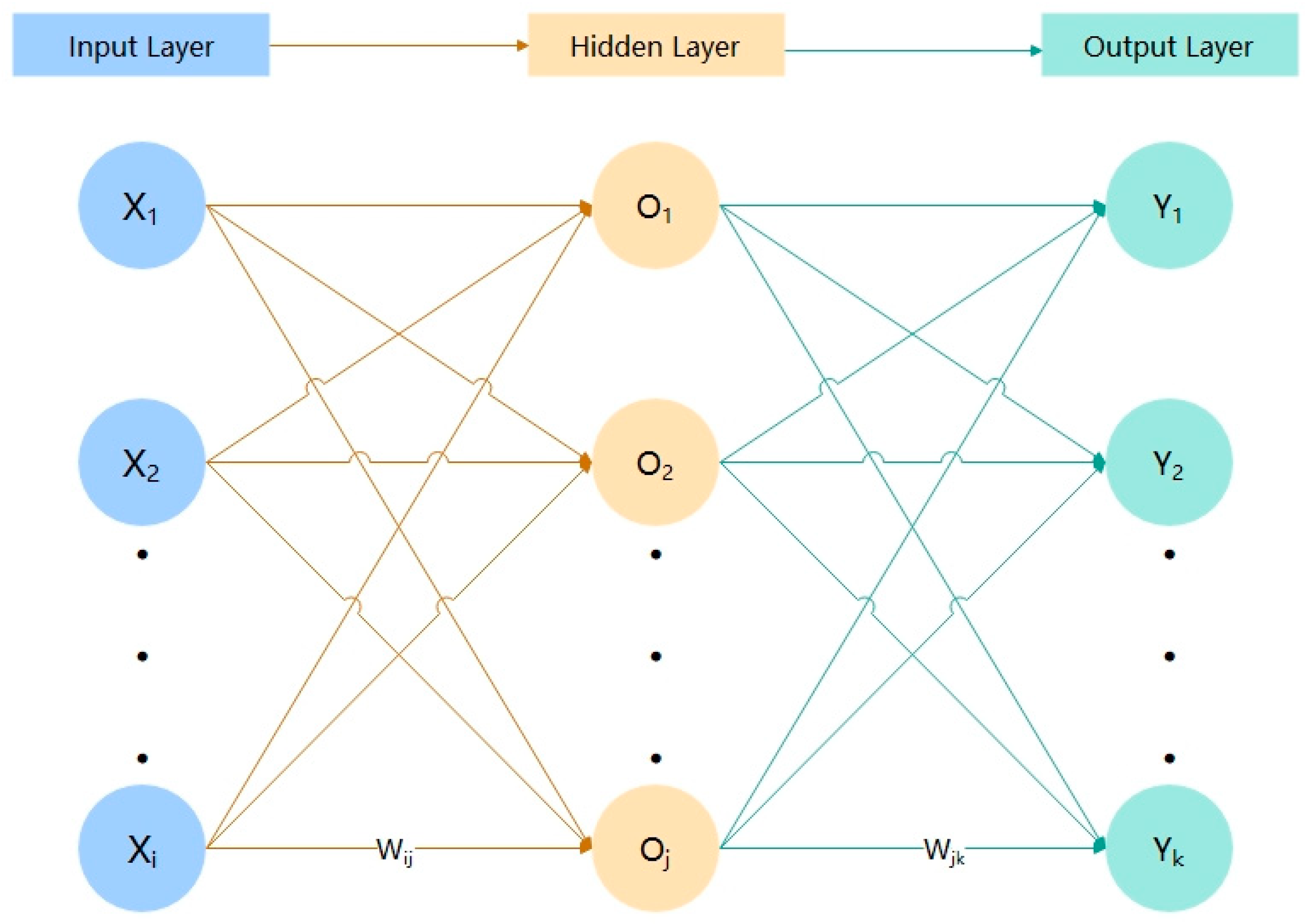
BPNN was proposed in 1986 by Rumelhart et al. [44]. The BPNN consists of an input layer, an implicit layer, and an output layer, which are trained by sample data. In addition, the network weights and thresholds are continuously modified and iterated until the minimum sum of squared errors of the network is reached, and the desired output is approximated. The topology of the three-layer BPNN is shown in Figure 1.
The input data are repeatedly fed into the neural network with feedback. Each time the data are repeated, the model compares the output of the neural network with the desired output and calculates the error. This error is back-propagated to the neural network and used to adjust the weights so that the error is reduced each time. Such a BPNN can get closer and closer to the desired output.
We perform global optimization for the cases containing one, two, and three hidden layers, and the number of neurons per layer is as follows. One hidden layer contains 10 neurons. The first of the two hidden layers contains 10 neurons and the second contains 20 neurons. In addition, the three hidden layers have three cases with the composition of neurons, and the number of neurons per layer is [10,10,10], [10,10,20], [10,20,30]. The Rectified Linear Unit (ReLU) activation function is a common neural activation function with sparsity. Therefore, this activation function is used in this paper to make the sparse model better able to mine relevant features to fit the training data. Global optimization is also performed for three optimizers which are mainly the limited memory Broyden–Fletcher–Goldfarb–Shanno (LBFGS), stochastic gradient descent (SGD), and adaptive moment estimation (ADAM).
3.2.4. Decision Trees (DT) and Random Forests (RF)
The regression decision tree mainly refers to the CART (Classification and Regression Tree) algorithm proposed by Breiman et al. in 1984 [45]. It mainly divides the feature space into several non-overlapping regions, and each division cell has a specific output. We can assign them to a cell according to the features and get the corresponding prediction value for the test data. The predicted value is the arithmetic mean of the values taken from each sample in the training set in that region.
RF is an integrated machine learning model consisting of several decision trees. When dealing with regression problems, N trees will have N outputs for one input sample, and the mean value of each decision tree output is the final output of the random forest.
In this paper, a global search is performed for the maximum depth of the tree and the number of features to be considered as branching when we apply the DT algorithm. In addition, the global search is performed for the number of base evaluators in the forest and the maximum depth of the tree when applying the RF algorithm.
3.2.5. Gradient Boosted Decision Tree (GBDT)
The GBDT algorithm, also called MART (Multiple Additive Regression Tree), is an iterative decision tree algorithm. The GBDT algorithm can be viewed as an additive model composed of M trees, and its corresponding equation is shown in Equation (6).
where x is the input sample, and w are the model parameters. h is the classification and regression tree; α is the weight of each tree.
The main idea of the algorithm is as follows. Firstly, the first base learner is initialized. Next, M base learners are created. The value of the negative gradient of the loss function in the current model is calculated and used as an estimate of the residual. Then, a CART regression tree is built to fit this residual, and a value that reduces the loss as much as possible is found at the leaf nodes of the fitted tree. Finally, the learner is updated.
In this paper, the mean squared loss function is used, and the number of trees in the parameters, the maximum depth as well as the learning rate are globally sought and tuned.
3.2.6. CatBoost, XGBoost, and LightGBM
CatBoost, XGBoost, and LightGBM can all be categorized into the family of gradient-boosting decision tree algorithms, and we describe the characteristics of the three models.
CatBoost combines category features to construct new features, which enriches the feature dimension and facilitates the model to find essential features.
XGBoost incorporates a regular term in the objective function to avoid the over-fitting of the model. At the same time, the model supports training and prediction for data containing missing values.
LightGBM takes GBDT as its core and makes essential improvements in many aspects, including second-order Taylor expansion for objective function optimization, a histogram algorithm, and an optimized leaf growth strategy. It makes the algorithm more efficient in training and more adaptable to high-dimensional data.
Global parameter search is performed for learning rate, number of trees, maximum depth, and sample rate in CatBoost, XGBoost, and LightGBM model parameters.
3.2.7. Adaboost and Bagging
Freund and Schapire proposed the Adaboost algorithm in 1997 [46]. The main idea is to assign an initial weight value to each sample for the same sample and then update the sample weight value by each iteration. The sample with a small error rate will have a reduced weight value in the next iteration, and the sample with significant error rate will boost the weight value in the next iteration. This algorithm belongs to a typical integrated learning method.
Bagging is another class of integrated learning methods. The main difference with Adaboost is that its training set is selected with put-back in the original set, and the training sets selected from the original set are independent of each other for each round. In addition, Adaboost determines the weight values based on the error rate situation, while Bagging uses uniform sampling with equal weights for each sample. Finally, the individual prediction functions of Bagging can be generated in parallel, while Adaboost can only generate them sequentially because the latter model parameters require the results of the previous model round.
In this paper, Adaboost uses decision trees as the weak evaluator, and the number of trees and learning rate are tuned to the parameters. The maximum depth of Bagging is 7, and the number of trees in the parameters is globally searched for.
4. Empirical Analysis
4.1. Design of the Empirical Analysis Process
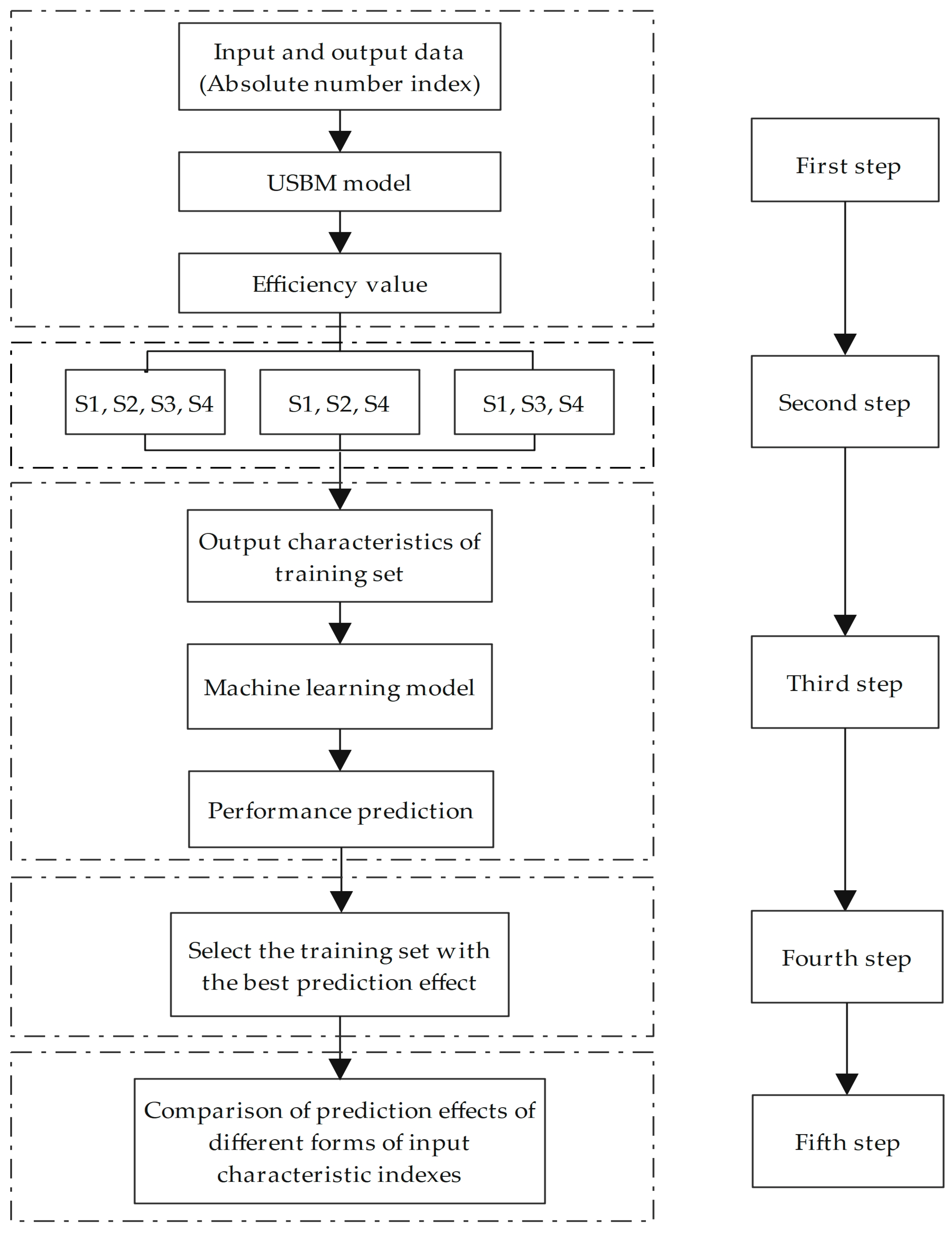
As shown in Figure 2, the steps of the empirical analysis based on the integrated DEA and machine learning model are as follows.
In the first step, based on the input and output indicators in the index system of carbon-emission efficiency, the SBM model with non-expected outputs in the DEA method is used to measure the efficiency values.
In the second step, the efficiency values obtained by the DEA model are classified into four categories of datasets, including S1, S2, S3, and S4. The four categories are classified using the quartile method, after which the prediction effects of the datasets under the three combinations of S1, S2, S3, S4, S1, S2, S4, and S1, S3, S4 classifications are compared.
In the third step, the efficiency values under the three combinations of classification in the second step are used as output feature indicators. The original input and output indicators are used as input feature indicators, and eleven machine learning methods are used for regression to find the optimal model.
In the fourth step, the machine learning models trained based on the three training sets under the DEA classification method are applied to the test set, to compare the prediction results and arrive at the training set with the best prediction results.
In the fifth step, the prediction effects of absolute number indicators and proportional relative indicators as machine learning input features are further analyzed.
4.2. Evaluation Index System Construction
The index system of carbon-emission efficiency evaluation is shown in Table 2. We selected labor force, capital stock, and total energy consumption as the three input indicators. The labor force indicator is the number of employed people in each province of China at the end of the year, and the unit is 10,000 people. The capital stock is selected as the real GDP of each year in each province of China, and the CPI data with 2006 as the base period is used to eliminate the effect of price changes in billion yuan. The energy variable is the total energy consumption of each province in China in a million tons of standard coal. GDP measures the expected output indicator in billions of yuan, and the GDP deflator is used to calculate the real GDP of each province in China excluding the effect of inflation. The non-desired output indicator is selected as the CO2 emissions of each Chinese province in tons.
4.3. Decision Units and Data Description
We selected 30 provinces in China as the decision unit, and the data are from 2006 to 2019. The data were obtained from the China Statistical Yearbook, China Energy Statistical Yearbook, China Provincial Statistical Yearbook, China Carbon Accounting Database, and the website of the National Bureau of Statistics of China. The data distribution of each input-output indicator is shown in Table 3.
4.4. Decision Unit Efficiency Value Measurement
In this paper, we use the Matlab software to construct a non-expectation and non-oriented SBM model to measure the carbon emission efficiency of thirty Chinese provinces, and the measurement results are shown in Table A1 of Appendix A. When the measurement result is equal to 1, the carbon emission is effective. Additionally, the smaller the value means, the lower the carbon emission efficiency of the province.
4.5. Evaluation Indicators of the Prediction Effect
We choose the coefficient of the wellness of the coefficient of determination (R2), Root Mean Squared Error (RMSE), and Mean Absolute Error (MAE) as the indicators to evaluate the prediction effect of the model.
R2 denotes the ratio of the explained sum of squares of deviations to the total sum of squares in the model, and the formula is expressed as Equation (7). is the actual value, denotes the predicted value, is the error from prediction, and is the error from the mean. The above parameters take constant values.
The RMSE is the square root of the sum of squares deviations of the observed values from the true values to the ratio of the number of observations m. The formula is expressed as Equation (8), representing the actual value and representing the predicted value. The above parameters take constant values.
MAE is the average absolute value of the error between the observed and true values, and the formula is expressed as Equation (9), representing the actual value and representing the predicted value. The above parameters take constant values.
Machine learning models with higher R2 and relatively lower RMSE as well as MAE means having better prediction results among the evaluation metrics.
For regression algorithms, R2 is the best measure of predictive effectiveness. This is because both RMSE and MAE have no upper and lower bounds. When our prediction model does not have any error, R2 will attain the maximum value of 1. When our model is equal to the benchmark model, R2 = 0. When R2 < 0, it means that the model we learned is not as good as the benchmark model.
The combined use of RMSE and MAE allows for the determination of anomalies in forecast errors. Specifically, MAE is a direct calculation of the mean value of the error. The MAE metric is not susceptible to extreme forecast values. The MAE focuses more on those forecast values that are close to the true value. The RMSE, on the other hand, indicates the degree of sample dispersion, which is sensitive to extreme errors. The extreme errors will make the value of RMSE much higher than the value of MAE. For instance, there are two datasets.
First set of data: True values [2, 4, 6, 8], predicted values [4, 6, 8, 10], MAE = 2.0, RMSE = 2.0.
Second set of data: True values [2, 4, 6, 8], predicted values [4, 6, 8, 12], MAE = 2.5, RMSE = 2.65.
From the results of both datasets, it can be observed that the RMSE is more sensitive than the MAE for the last predicted value. Usually, the RMSE is greater than or equal to the MAE. The only case where the RMSE is equal to the MAE is when all errors are equal or all are zero, such as the one shown in the first set. This case can be used as a reference for model users. If a model with smooth prediction errors is desired, then, a model with an RMSE that is closer to the MAE at a larger R2 can be chosen.
4.6. Performance Prediction Based on DEA and Machine Learning Models
This paper plans to include input-output indicators of Chinese provinces from 2006 to 2018 as input feature indicators and efficiency values as output feature indicators in the training set to learn them using eleven machine learning models. Then, we select the efficiency values of each Chinese province in 2019 as the prediction object to test the prediction effect.
Before prediction, we normalize the input characteristic index data. Since the output index is the efficiency value which falls within the interval of 0 to 1, no normalization is required.
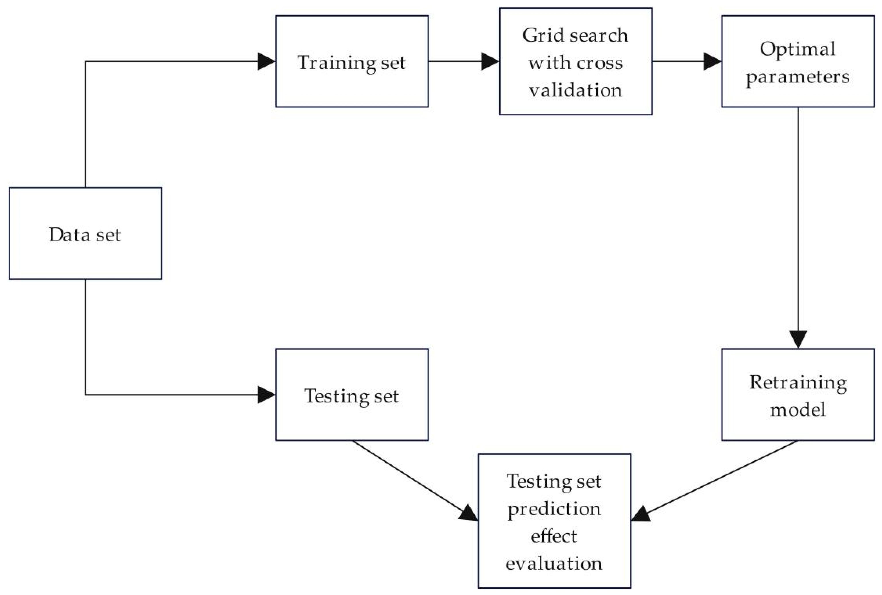
In the hyperparameter selection, we search for the optimal hyperparameters by grid search and use multiple hyperparameters for simultaneous optimization. Currently, some individual hyperparameters are tuned, and other hyperparameters will take default values. It ignores the combined effect of multiple hyperparameters on the model. Therefore, this paper uses multiple hyperparameters for simultaneous optimization. In order to avoid the over-fitting of hyperparameters, each group of hyperparameters is evaluated using cross-validation combined with five-fold cross-validation. Finally, hyperparameters with the best cross-validation performance are selected to fit a new model, and the model hyperparameter search and prediction process is shown in Figure 3.
Based on the training set of all sample data from 30 Chinese provinces from 2006 to 2018, the prediction results of the test set using the 30 Chinese province samples in 2019 were derived as shown in Table A2 of Appendix A. According to the results, the average R2, RMSE, and MAE are 0.8409, 0.1348, and 0.0941, respectively. Sorting by R2, we can find that the five models with the best prediction results are BPNN, CatBoost, XGBoost, GBDT, and LightGBM. By calculating the ratio of RMSE to MAE, it can be found that the ratio of GBDT is the highest among the five models at 1.7165. This indicates that its prediction error is most prone to abnormal values. The models with poor prediction results mainly include linear regression model and decision tree model and AdaBoost, and their R2 is less than 0.8.
4.7. Results of the Empirical Study Based on the Training Subset of DEA Classification Method
After using the full sample data for training, the authors of this paper pose a research question: which of the more valid sample data or relatively invalid sample data can be more effective in improving the prediction? So, we proposed the DEA classification method. This paper uses the quartile method to classify the efficiency values based on the measured efficiency values. Based on this, this paper further classifies the efficiency value intervals S1[0.6284, 1], S2[0.4309, 0.6284), S3[0.3541, 0.4309), and S4[0, 0.3541). It is empirically known that S1 and S4 intervals are the most effective interval and the least effective interval, respectively, which will provide the most feature information for model training. Then, as the more effective sample dataset S2 and the relatively ineffective sample dataset S3, one can ask: which one contributes more? This paper compares the prediction effects of S1, S2, and S4 as training sets and S1, S3, and S4 as training sets. The detailed results are shown in Table A3 and Table A4 of Appendix A.
The five models with the best prediction results based on the S1, S2, and S4 training sets are BPNN, XGBoost, CatBoost, LightGBM, and GBDT. The five models with the best prediction results based on the S1, S3, and S4 training sets are CatBoost, BPNN, XGBoost, LightGBM, and SVR. The average R2, RMSE, and MAE of S1, S2, and S4 training sets are 0.8461, 0.1355, and 0.0980, respectively. The average R2, RMSE, and MAE of S1, S3, and S4 training sets are 0.8150, 0.1496, and 0.1054, respectively. It can be seen that S1, S2, and S4 training sets have better results than S1, S3, and S4 training sets in terms of R2, RMSE, and MAE. Therefore, the S1, S2, and S4 training sets are significantly better than the S1, S3, and S4 training sets. Additionally, it can be inferred that the more effective sample data have more excellent value and will provide more feature information for model training, thus effectively improving the prediction effect of the model.
Among the machine learning models based on S1, S2, and S4 training sets, only LightGBM and Bagging are less effective than the models based on S1, S3, and S4 training sets in terms of prediction effects. The difference between the prediction results of the LightGBM model on S1, S2, S4 and S1, S3, S4 training sets is small. And this is also the case for the Bagging model. The prediction effect of Linear Regression and SVR is the same. Seven models have significantly higher prediction effects in S1, S2, and S4 training sets than in S1, S3, and S4 training sets when comparing R2, RMSE, and MAE evaluation metrics. This would further prove the robustness of the conclusions drawn by the authors.
4.8. Results of the Empirical Study of Proportional Relative and Absolute Number Indicators
In this paper, the authors consider that the output characteristics are efficiency values under the DEA method, i.e., the ratio of weighted outputs to weighted inputs. If the input characteristic variables are transformed into the ratio of output indicators to input indicators, their predictive effects may be better than absolute number indicators. Based on this assumption, this paper further verified it.
First, based on the results of the empirical study based on the training subsets of the DEA classification method, the training sets S1, S2, and S4 with the best prediction results were selected and used for further research.
Further, the input characteristics indicators are adjusted to GDP/labor, GDP/capital stock, GDP/energy, (1/CO2 emissions)/labor, (1/CO2 emissions)/capital stock, and (1/CO2 emissions)/energy. In addition, CO2 emissions are taken as the reciprocal as a non-desired output indicator, which is more consistent with the definition of efficiency values under the DEA approach than the upper input indicators.
The prediction effect based on proportional relative index of the eleven machine learning models are shown in Table A5 of Appendix A. The average R2, average RMSE, and average MAE of the eleven machine learning models significantly improve the prediction performance compared to the absolute number of indicators in Table A3 of Appendix A. Nine of the models outperformed the absolute number indicators based on proportional relative indicators. The R2 of XGBoost is 0.9721, and the values of RMSE and MAE are 0.0553 and 0.0409, respectively. The authors’ hypothesis that the proportional relative indicators have a better prediction effect than the absolute number indicators was proved.
Based on Section 4.6 and Section 4.7, ranking the R2 metrics in three different datasets for each machine learning model by taking the mean value, or by taking the mean value for each ranking, we can get the same results. The results showed that the five models with the best prediction results were ranked as BPNN, CatBoost, XGBoost, LightGBM, and GBDT. Figure 4 shows the detailed prediction of the five models under the proportional relative index and absolute number index. GBDT represents the GBDT model under the absolute number metric, GBDT-PRI represents the GBDT model under the relative proportional metric, and the other four models are also labeled in the same way. To show the results more intuitively, R2 is shown as 100 times the original value, the average RMSE is shown as 1000 times the original value, and the average MAE is shown as 1000 times the original value in the pictures. Based on the histogram comparison, it can be more clearly seen that the model prediction based on proportional relative indicators outperforms the model prediction based on absolute number indicators.
4.9. Analysis of Errors
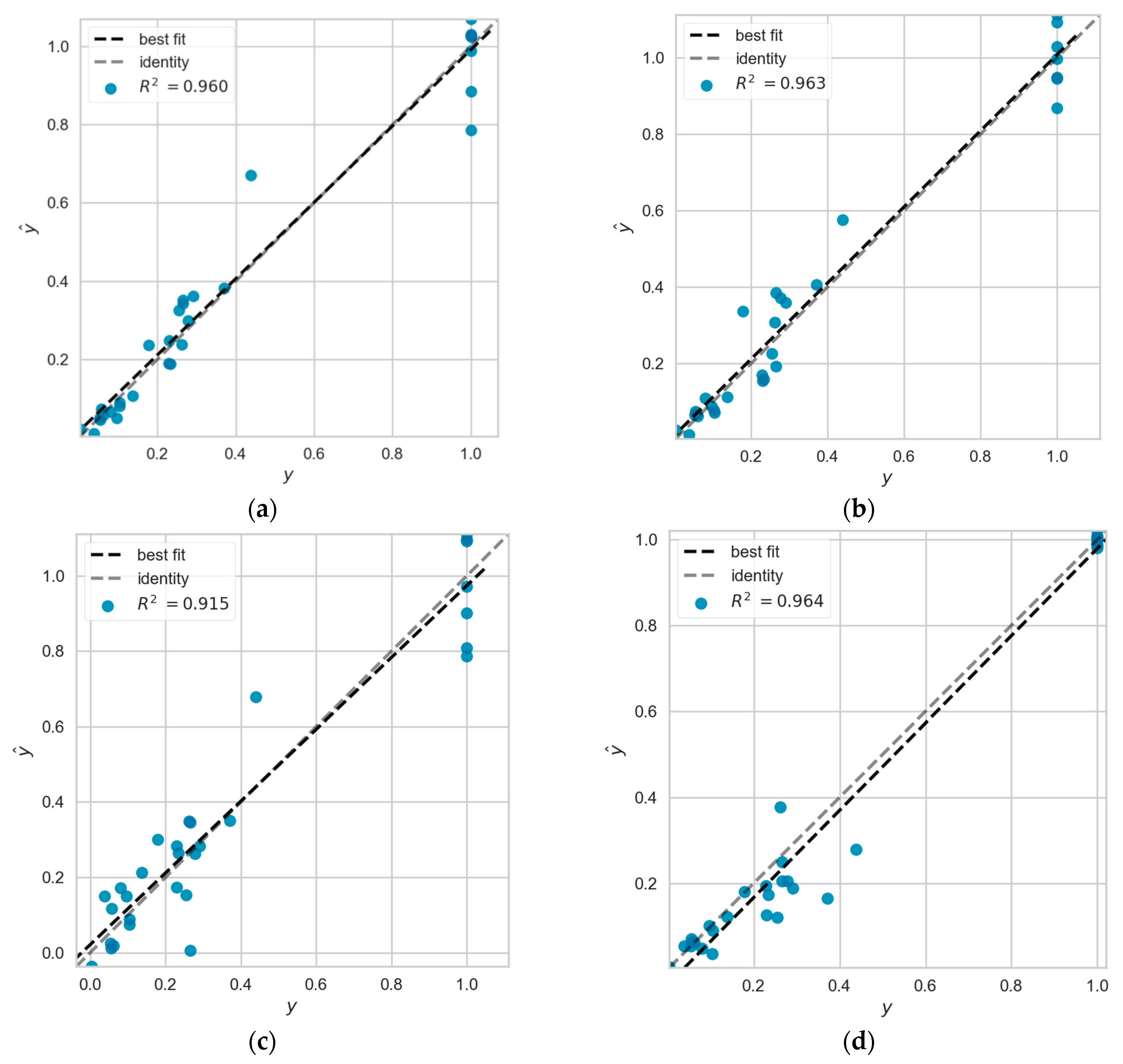
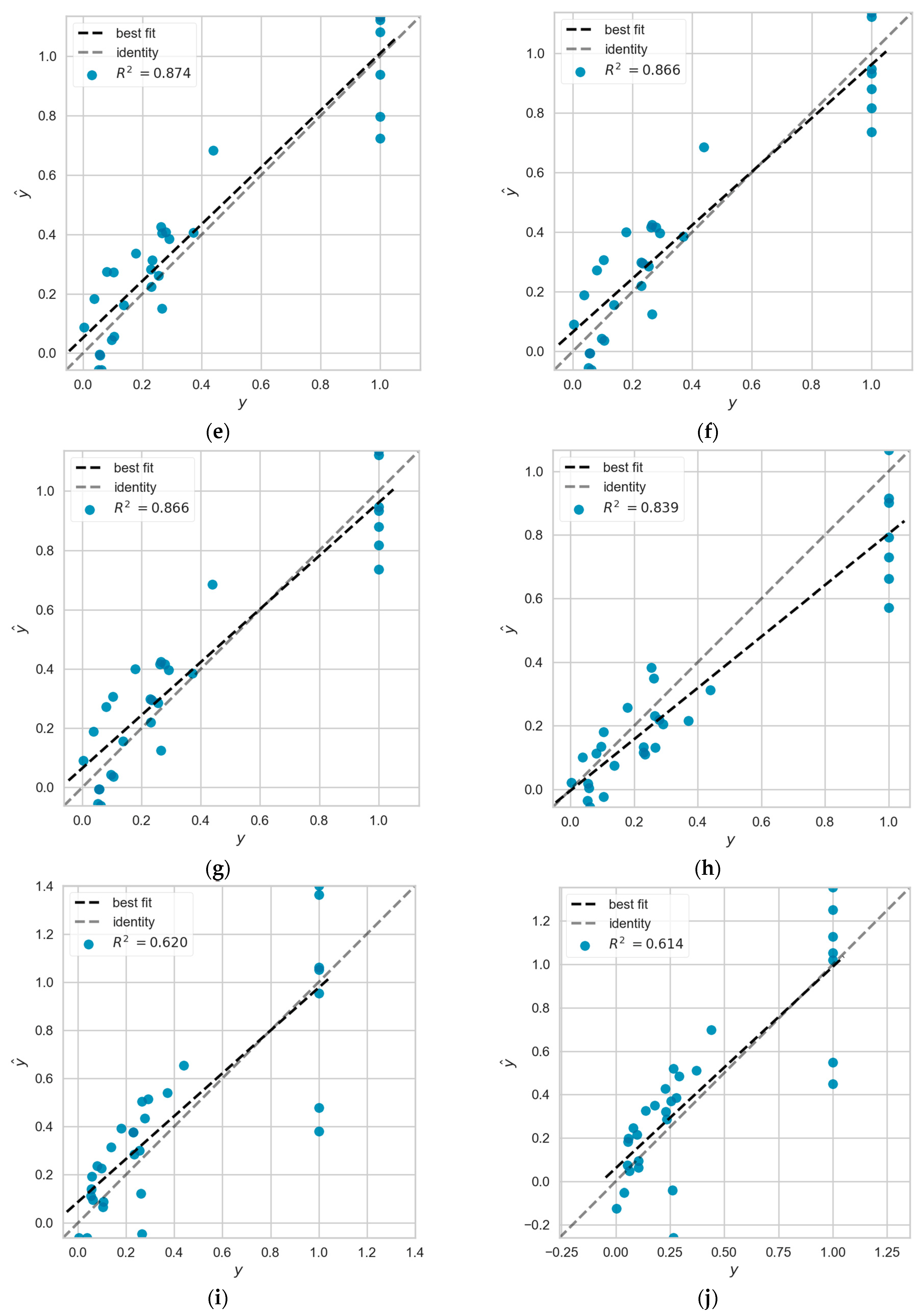
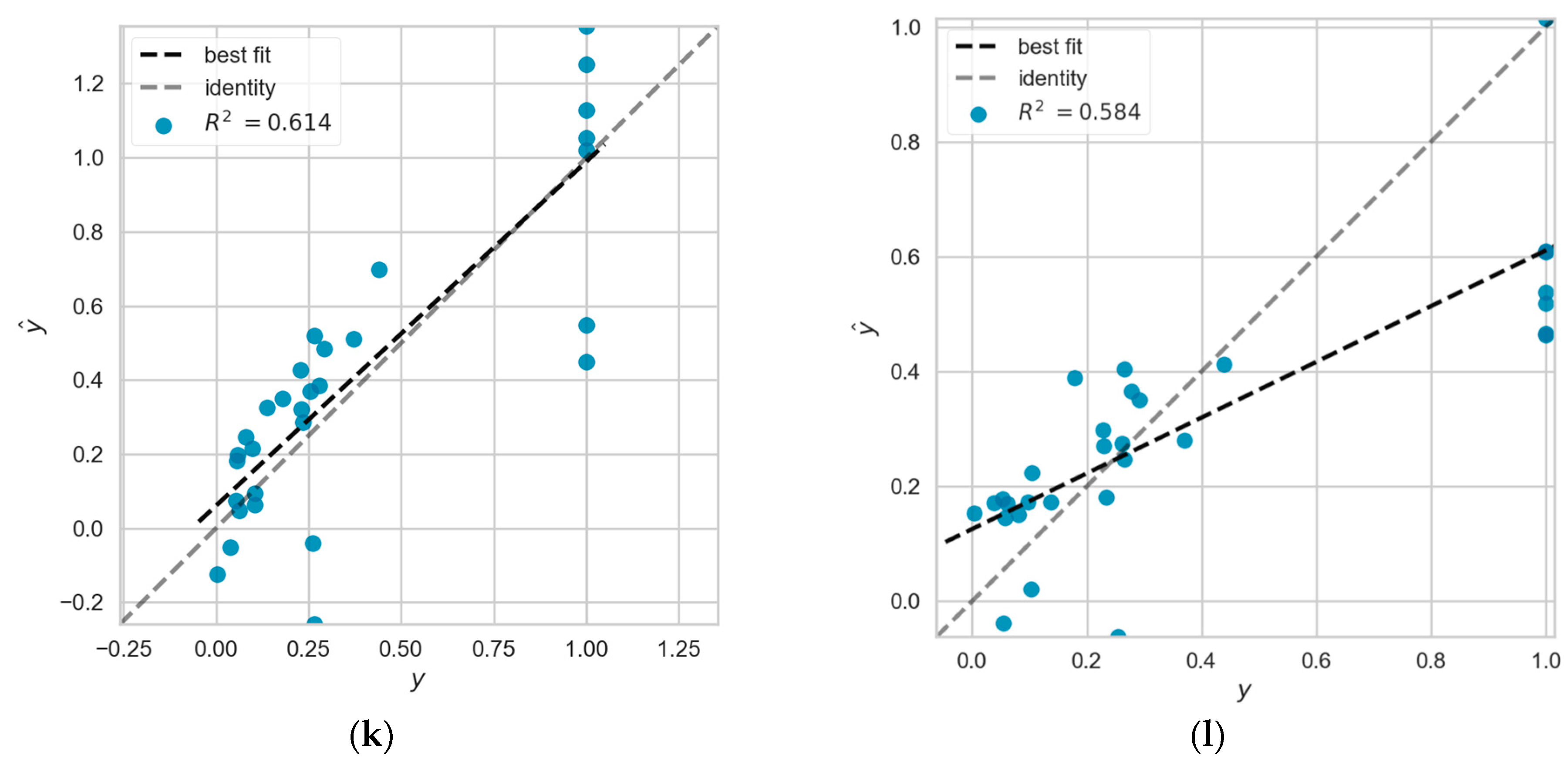
This section ranks each model by calculating the average R2 of the eleven models over the four predictions. We selected the model ranked first, the model ranked in the middle (sixth place), and the model ranked last. They are the BPNN model, the SVR model, and the LR model, respectively. We plotted the prediction errors of the above three models for the four predictions. The figure is shown in Figure A1 of Appendix A, and is combined with empirical data for further error analysis.
We first perform a comparative analysis of the performance of the BPNN, SVR, and LR models in each of the four predictions. Subsequently, we perform a comparative analysis based on the performance of different models in the same prediction. We found that the BPNN model has higher R2 based on absolute number index and proportional relative index in S1, S2, and S4 training sets with 0.9630 and 0.9638, respectively. The absolute minimum prediction errors are 0.0007 and 0.0003, and the absolute maximum prediction errors are 0.1583 and 0.2059. Although the absolute minimum prediction errors are similar, the absolute maximum prediction errors are much different. The model with higher R2 has a larger absolute maximum prediction error. We further compare the predicted and actual values in the test set. It is found that the main reason for this phenomenon is that the BPNN model has abnormal prediction error values in S1, S2, and S4 training sets based on the proportional relative index. Its mean error value is smaller than the mean error value of BPNN model in absolute number index, and 66.67% of the errors are smaller than the mean error value, which is 6.67% higher than the latter. It can also be concluded from the ratio of RMSE and MAE that the former ratio is greater than the latter. This indicates that the presence of anomalous prediction error values leads to an increase in the ratio, because the RMSE has a more sensitive reflection of the anomalous prediction error values.
The R2 of the SVR model was similar in three of the four predictions, 0.8743, 0.8658, and 0.8658, respectively, and the RMSE and MAE ratios of these three predictions were 1.1611 to 1.1621. The mean prediction error, the absolute minimum prediction error, and the absolute maximum prediction error were also similar. The worst prediction result was compared with the three good prediction results, and the average prediction error of 0.1143 was only 0.0039 higher than that of the lowest average prediction error, but the absolute maximum prediction error was 0.4286, which was much higher than the other three. This leads to a decrease in the fit of the model, and the ratio of RMSE to MAE helps us to confirm this.
The LR model, as the worst prediction model, has the maximum value of absolute maximum prediction error exceeding 0.5 in all four predictions. The prediction error diagram reveals that its error distribution based on proportional relative index on S1, S2, and S4 training sets is significantly different from the other three times. The main reason is that the average prediction error reaches 0.3357 for the samples with actual output value of 1. There are four sample points with prediction values between 0.4 and 0.6, which are significantly more than the other three predictions. Therefore, it has the lowest R2 among the four predictions, and the ratio of RMSE and MAE is also greater than the other three.
In addition, the average prediction error, absolute maximum prediction error and absolute minimum prediction error of the BPNN model are better than those of the SVR and LR models in the four predictions. The average prediction error and the absolute maximum prediction error of the SVR model were also better than those of the LR model in the four predictions. The absolute number index-based absolute minimum prediction error on S1, S2, and S4 training sets and S1, S3, and S4 training sets showed higher prediction error for the SVR model though, which was 0.0002 and 0.0004 higher than that of the LR model, respectively. In the case that the average prediction error and the absolute maximum prediction error are significantly better than those of the LR model, there is no excessive effect on the overall prediction effect of the SVR model.
5. Results and Discussion
As a result of the empirical study, we have achieved the following three results.
- (1)
- In this paper, the absolute efficient frontier is constructed and applied to the performance prediction of a new decision unit. It can break through the limitations of the DEA method, which is based on the input-output index data of the decision unit to constitute the production frontier surface. This frontier surface is relative, and changes as new decision units are added to the frontier surface. The application of the new method allows the addition of new decision units at any time without changing the effective frontier surface and completes a comparative study of the old and new decision units. In addition, the radial or non-radial DEA model measures the efficiency values of each decision unit for each year based on cross-sectional data. Technical efficiency changes and technological progress mainly dominate the variation of efficiency values between years. The radial or non-radial DEA model cannot compare the technical efficiency changes in different years. Using the absolute efficient frontier, the cross-sectional limitation can be broken, and the technical efficiency situation of each decision unit in each year can be compared.
- (2)
- Based on the efficiency scores measured by the DEA method, the efficiency scores are classified by the quartiles method, and then, the different categories are combined and used to train a variety of machine learning models. The trained machine learning models can be used to predict the efficiency scores of new decision units, and the analysis combined with the fitting effect can lead to two conclusions: (i) more effective sample data provide more important feature information; (ii) relatively ineffective sample data will bring the noise to the model learning.
- (3)
- Based on the results of the empirical study of the training subset of the DEA classification method, the training subset with the best prediction effect was selected and used to study further the prediction effect of proportional relative indicators and absolute number indicators. After the empirical study, it was found that the proportional relative index has a better prediction effect compared with the absolute number index.
Of course, we need to know that performance prediction can be improved by feature engineering. This paper does not discuss several methodological techniques for the data preparation as well as investigate the effect of different taxonomies of datasets on prediction effectiveness, which are subject to further development.
6. Conclusions
In this paper, we propose a performance prediction method based on the SBM model in the DEA method combined with eleven machine learning models. To verify the rationality of the model approach, we forecast the carbon emission efficiency of 30 Chinese provinces in 2019 to compare the results with the DEA calculation. Good prediction results are achieved and the performance prediction of new decision units without changing the leading edge is achieved. The situation that DEA cannot predict the performance of new decision units is solved. Based on the performance prediction achieved by the integrated model of DEA and machine learning, we further propose improving the model’s prediction accuracy in terms of training set sample selection and input feature indicators. Through empirical research, we found that “valid” data in DEA can provide more important characteristic information than “invalid” data. In addition, the use of proportional relative indicators gained more accurate prediction values than absolute number indicators.
In summary, the relationship between efficiency values and input-output variables is complex and nonlinear. Moreover, machine learning models have unique advantages for solving nonlinear problems. The proposed integrated model of data envelopment analysis and machine learning provides a new idea for the feasibility study for performance evaluation and prediction. This paper takes carbon emission performance prediction as an example and achieves good prediction results. Currently, our study has some limitations for further research in the future. These include: (1) only the discriminative effect of the integrated model of DEA and machine learning on the regression problem is considered, and the classification problem is not explored. (2) This paper integrates eleven machine learning models and SBM models commonly used in DEA methods, and further expansion of the base models in this integrated model is needed. (3) It should be extended to a wider range of applications. (4) The running time of the algorithm is long, how to further simplify the complexity of the model and improve the running efficiency of the model is the future research direction.
Author Contributions
Conceptualization, Z.Z.; methodology, Z.Z., Y.X. and H.N.; writing—original draft preparation, Z.Z., Y.X. and H.N.; writing—review and editing, Z.Z., Y.X. and H.N. All authors have read and agreed to the published version of the manuscript.
Funding
This research was supported by Beijing Foreign Studies University Double First Class Major Landmark Project (No. 2022SYLZD001) in China, and the Fundamental Research Funds for the Central Universities (No. 2022JX031) in China.
Institutional Review Board Statement
Not applicable.
Informed Consent Statement
Not applicable.
Data Availability Statement
The data of this study can be obtained by contacting the author, email address: [email protected].
Conflicts of Interest
The authors declare no conflict of interest.
Appendix A

Table A1.
Results of carbon emission efficiency in 30 Chinese provinces from 2006 to 2019.
| Provincial Area | 2006 | 2007 | 2008 | 2009 | 2010 | 2011 | 2012 | 2013 | 2014 | 2015 | 2016 | 2017 | 2018 | 2019 |
|---|---|---|---|---|---|---|---|---|---|---|---|---|---|---|
| Anhui | 0.52 | 0.51 | 0.47 | 0.45 | 0.45 | 0.44 | 0.43 | 0.41 | 0.40 | 0.40 | 0.40 | 0.41 | 0.41 | 0.41 |
| Beijing | 1.00 | 1.00 | 1.00 | 1.00 | 1.00 | 1.00 | 1.00 | 1.00 | 1.00 | 1.00 | 1.00 | 1.00 | 1.00 | 1.00 |
| Chongqing | 0.50 | 0.51 | 0.48 | 0.48 | 0.50 | 0.50 | 0.52 | 0.56 | 0.56 | 0.57 | 0.57 | 0.61 | 0.60 | 0.59 |
| Fujian | 0.63 | 0.59 | 0.58 | 0.54 | 0.53 | 0.51 | 0.52 | 0.53 | 0.52 | 0.51 | 0.52 | 0.56 | 0.55 | 0.54 |
| Gansu | 0.40 | 0.40 | 0.39 | 0.39 | 0.39 | 0.40 | 0.41 | 0.41 | 0.42 | 0.43 | 0.43 | 0.43 | 0.44 | 0.44 |
| Guangdong | 1.00 | 1.00 | 1.00 | 1.00 | 1.00 | 1.00 | 1.00 | 1.00 | 1.00 | 1.00 | 1.00 | 1.00 | 1.00 | 1.00 |
| Guangxi | 0.49 | 0.47 | 0.22 | 0.44 | 0.39 | 0.31 | 0.31 | 0.32 | 0.32 | 0.32 | 0.32 | 0.32 | 0.35 | 0.31 |
| Guizhou | 0.29 | 0.31 | 0.32 | 0.32 | 0.32 | 0.32 | 0.32 | 0.32 | 0.33 | 0.33 | 0.33 | 0.33 | 0.33 | 0.32 |
| Hainan | 1.00 | 1.00 | 1.00 | 1.00 | 1.00 | 1.00 | 1.00 | 1.00 | 1.00 | 1.00 | 1.00 | 1.00 | 1.00 | 1.00 |
| Hebei | 0.37 | 0.25 | 0.28 | 0.28 | 0.28 | 0.28 | 0.28 | 0.29 | 0.29 | 0.30 | 0.31 | 0.28 | 0.35 | 0.28 |
| Henan | 0.46 | 0.44 | 0.44 | 0.41 | 0.39 | 0.38 | 0.39 | 0.31 | 0.39 | 0.40 | 0.40 | 0.43 | 0.44 | 0.47 |
| Heilongjiang | 0.44 | 0.42 | 0.41 | 0.38 | 0.37 | 0.29 | 0.37 | 0.36 | 0.37 | 0.35 | 0.35 | 0.37 | 0.37 | 0.38 |
| Hubei | 0.41 | 0.40 | 0.27 | 0.40 | 0.40 | 0.39 | 0.39 | 0.40 | 0.42 | 0.43 | 0.43 | 0.44 | 0.44 | 0.44 |
| Hunan | 0.47 | 0.45 | 0.44 | 0.43 | 0.41 | 0.40 | 0.41 | 0.42 | 0.43 | 0.44 | 0.44 | 0.46 | 0.35 | 0.49 |
| Jilin | 0.21 | 0.37 | 0.29 | 0.29 | 0.30 | 0.30 | 0.30 | 0.31 | 0.32 | 0.32 | 0.32 | 0.34 | 0.35 | 0.35 |
| Jiangsu | 0.71 | 0.72 | 0.74 | 0.78 | 1.00 | 1.00 | 1.00 | 1.00 | 1.00 | 1.00 | 1.00 | 1.00 | 1.00 | 1.00 |
| Jiangxi | 0.52 | 0.52 | 0.52 | 0.51 | 0.50 | 0.49 | 0.51 | 0.48 | 0.49 | 0.48 | 0.47 | 0.48 | 0.47 | 0.47 |
| Liaoning | 0.41 | 0.39 | 0.36 | 0.31 | 0.31 | 0.31 | 0.32 | 0.32 | 0.32 | 0.32 | 0.33 | 0.33 | 0.34 | 0.33 |
| Inner Mongolia | 0.40 | 0.38 | 0.37 | 0.35 | 0.31 | 0.32 | 0.32 | 0.32 | 0.33 | 0.33 | 0.34 | 0.34 | 0.34 | 0.35 |
| Ningxia | 0.64 | 0.63 | 1.00 | 0.59 | 0.59 | 0.59 | 0.61 | 0.48 | 0.49 | 0.48 | 0.47 | 0.45 | 0.46 | 0.46 |
| Qinghai | 1.00 | 1.00 | 1.00 | 1.00 | 1.00 | 1.00 | 1.00 | 1.00 | 1.00 | 1.00 | 1.00 | 1.00 | 1.00 | 1.00 |
| Shandong | 0.44 | 0.43 | 0.42 | 0.42 | 0.41 | 0.42 | 0.42 | 0.44 | 0.44 | 0.43 | 0.44 | 0.46 | 0.46 | 0.47 |
| Shanxi | 0.40 | 0.39 | 0.28 | 0.28 | 0.29 | 0.29 | 0.29 | 0.30 | 0.30 | 0.30 | 0.31 | 0.29 | 0.35 | 0.30 |
| Shaanxi | 0.41 | 0.40 | 0.27 | 0.39 | 0.38 | 0.37 | 0.36 | 0.36 | 0.35 | 0.35 | 0.35 | 0.35 | 0.35 | 0.35 |
| Shanghai | 1.00 | 1.00 | 1.00 | 1.00 | 1.00 | 1.00 | 1.00 | 1.00 | 1.00 | 1.00 | 1.00 | 1.00 | 1.00 | 1.00 |
| Sichuan | 0.43 | 0.40 | 0.38 | 0.38 | 0.39 | 0.41 | 0.42 | 0.43 | 0.43 | 0.45 | 0.45 | 0.48 | 0.48 | 0.48 |
| Tianjin | 0.66 | 0.63 | 0.63 | 0.61 | 0.55 | 0.54 | 0.54 | 0.52 | 0.52 | 0.53 | 0.53 | 0.45 | 0.45 | 0.45 |
| Xinjiang | 0.41 | 0.42 | 0.42 | 0.41 | 0.40 | 0.39 | 0.38 | 0.36 | 0.32 | 0.32 | 0.33 | 0.32 | 0.35 | 0.32 |
| Yunnan | 0.40 | 0.23 | 0.39 | 0.39 | 0.38 | 0.36 | 0.32 | 0.33 | 0.33 | 0.34 | 0.34 | 0.32 | 0.35 | 0.32 |
| Zhejiang | 0.70 | 0.68 | 0.69 | 0.70 | 0.71 | 0.72 | 0.73 | 0.72 | 0.74 | 0.74 | 0.74 | 0.76 | 1.00 | 1.00 |
Table A2.
Prediction effect of the test set based on the training set of all sample data.
| R2 | RMSE | MAE | Ranking | |
|---|---|---|---|---|
| Linear Regression | 0.6203 | 0.2231 | 0.1704 | 10 |
| GBDT | 0.9157 | 0.1051 | 0.0612 | 4 |
| XGBoost | 0.9396 | 0.0890 | 0.0630 | 3 |
| LightGBM | 0.9021 | 0.1133 | 0.0812 | 5 |
| CatBoost | 0.9479 | 0.0826 | 0.0611 | 2 |
| AdaBoost | 0.7598 | 0.1774 | 0.1534 | 9 |
| SVR | 0.8743 | 0.1283 | 0.1104 | 7 |
| BPNN | 0.9601 | 0.0723 | 0.0483 | 1 |
| Decision Trees | 0.5877 | 0.2324 | 0.0976 | 11 |
| Random Forest | 0.8875 | 0.1214 | 0.0882 | 6 |
| Bagging | 0.8549 | 0.1379 | 0.1007 | 8 |
| Average Value | 0.8409 | 0.1348 | 0.0941 |
Table A3.
Prediction effect of test set based on S1, S2, and S4 training sets.
| R2 | RMSE | MAE | Ranking | |
|---|---|---|---|---|
| Linear Regression | 0.6145 | 0.2248 | 0.1754 | 11 |
| GBDT | 0.8696 | 0.1307 | 0.0782 | 5 |
| XGBoost | 0.9401 | 0.0886 | 0.0643 | 2 |
| LightGBM | 0.8738 | 0.1286 | 0.0886 | 4 |
| CatBoost | 0.9401 | 0.0886 | 0.0653 | 3 |
| AdaBoost | 0.7328 | 0.1871 | 0.1609 | 10 |
| SVR | 0.8658 | 0.1326 | 0.1142 | 6 |
| BPNN | 0.9630 | 0.0697 | 0.0550 | 1 |
| Decision Trees | 0.8459 | 0.1421 | 0.0598 | 7 |
| Random Forest | 0.8365 | 0.1464 | 0.1051 | 8 |
| Bagging | 0.8248 | 0.1515 | 0.1110 | 9 |
| Average Value | 0.8461 | 0.1355 | 0.0980 |
Table A4.
Prediction effect of test set based on S1, S3, and S4 training sets.
| R2 | RMSE | MAE | Ranking | |
|---|---|---|---|---|
| Linear Regression | 0.6145 | 0.2248 | 0.1754 | 11 |
| GBDT | 0.8561 | 0.1373 | 0.0728 | 6 |
| XGBoost | 0.9121 | 0.1073 | 0.0761 | 3 |
| LightGBM | 0.8828 | 0.1239 | 0.0837 | 4 |
| CatBoost | 0.9377 | 0.0903 | 0.0638 | 1 |
| AdaBoost | 0.6692 | 0.2082 | 0.1568 | 10 |
| SVR | 0.8658 | 0.1326 | 0.1142 | 5 |
| BPNN | 0.9148 | 0.1057 | 0.0833 | 2 |
| Decision Trees | 0.6810 | 0.2045 | 0.1129 | 9 |
| Random Forest | 0.8050 | 0.1599 | 0.1105 | 8 |
| Bagging | 0.8257 | 0.1511 | 0.1104 | 7 |
| Average Value | 0.8150 | 0.1496 | 0.1054 |
Table A5.
Prediction effects based on proportional relative indicators.
| R2 | RMSE | MAE | |
|---|---|---|---|
| Linear Regression | 0.5836 | 0.2336 | 0.1673 |
| GBDT | 0.9359 | 0.0917 | 0.0573 |
| XGBoost | 0.9721 | 0.0553 | 0.0409 |
| LightGBM | 0.9616 | 0.0709 | 0.0491 |
| CatBoost | 0.9674 | 0.0654 | 0.0449 |
| AdaBoost | 0.9246 | 0.0994 | 0.0684 |
| SVR | 0.8394 | 0.1450 | 0.1143 |
| BPNN | 0.9638 | 0.0688 | 0.0438 |
| Decision Trees | 0.9324 | 0.0941 | 0.0640 |
| Random Forest | 0.8875 | 0.1214 | 0.0882 |
| Bagging | 0.9020 | 0.1133 | 0.0792 |
| Average Value | 0.8973 | 0.1054 | 0.0743 |
Table A6.
Explanation of parameters contained in formulas.
| Parameter | Affiliation Formula | Formula Belongs to the Model | Parameter Description | Range of Values |
|---|---|---|---|---|
| Equation (1) Equation (2) Equation (3) | CCR model BCC model | Each decision unit has m kind of input | ||
| Equation (1) Equation (2) Equation (3) | CCR model BCC model | Each decision unit has q kind of output | R | |
| Equation (1) | CCR model | The weight of the input | ||
| Equation (1) | CCR model | The weight of the output | ||
| θ | Equation (2) Equation (3) | CCR model BCC model | Efficiency value | |
| λ | Equation (2) Equation (3) | CCR model BCC model | The linear combination coefficient of the decision unit | |
| Equation (4) | SBM model | Objective function | ||
| Equation (4) | SBM model | Input slack variable | ||
| Equation (4) | SBM model | Desired output slack variable | ||
| Equation (4) | SBM model | Non-desired output slack variable | ||
| Equation (5) | Linear Regression | Input vector | R | |
| Equation (5) | Linear Regression | Output vector | R | |
| Equation (5) | Linear Regression | Linear mapping from input to output (Weight matrix) | R | |
| b | Equation (5) | Linear Regression | Offset items | C |
| x | Equation (6) | GBDT model | Input sample | R |
| w | Equation (6) | GBDT model | Weighting factor | R |
| M | Equation (6) | GBDT model | The dataset is divided into M cells | |
| Equation (6) | GBDT model | CART regression tree function | R | |
| α | Equation (6) | GBDT model | Weighting factor for each regression tree | |
| R2 | Equation (7) | Predictive effectiveness evaluation model | Coefficient of determination | |
| Equation (7) Equation (8) Equation (9) | Predictive effectiveness evaluation model | Actual value | R | |
| Equation (7) Equation (8) Equation (9) | Predictive effectiveness evaluation model | Predicted value | R | |
| m | Equation (8) Equation (9) | Predictive effectiveness evaluation model | The number of observations |
Figure A1.
(a–c) Prediction error diagram of BPNN model based on absolute number index on S1, S2, S3, S4 training set, S1, S2, S4 training set, S1, S3, S4 training set; (d) prediction error diagram of linear regression model based on proportional relative index on S1, S2, S4 training sets; (e–g) prediction error diagram of SVR model based on absolute number index on S1, S2, S3, S4 training sets, S1, S2, S4 training sets, S1, S3, S4 training sets; (h) prediction error diagram of SVR model based on proportional relative index on S1, S2, S4 training sets; (i–k) prediction error diagram of LR model based on absolute number index on S1, S2, S3, S4 training sets, S1, S2, S4 training sets, S1, S3, S4 training sets; (l) prediction error diagram of LR model based on proportional relative index on S1, S2, S4 training set.


References
- Charnes, A.; Cooper, W.W.; Rhodes, E. Measuring the efficiency of decision making units. Eur. J. Oper. Res. 1978, 2, 429–444. [Google Scholar] [CrossRef]
- Staub, R.B.; Souza, G.D.; Tabak, B.M. Evolution of bank efficiency in Brazil: A DEA approach. Eur. J. Oper. Res. 2010, 202, 204–213. [Google Scholar] [CrossRef]
- Holod, D.; Lewis, H.F. Resolving the deposit dilemma: A new DEA bank efficiency model. J. Bank. Financ. 2011, 35, 2801–2810. [Google Scholar] [CrossRef]
- Titko, J.; Stankevičienė, J.; Lāce, N. Measuring bank efficiency: DEA application. Technol. Econ. Dev. Econ. 2014, 20, 739–757. [Google Scholar] [CrossRef]
- Kamarudin, F.; Sufian, F.; Nassir, A.M.; Anwar, N.A.; Hussain, H.I. Bank efficiency in Malaysia a DEA approach. J. Cent. Bank. Theory Pract. 2019, 1, 133–162. [Google Scholar] [CrossRef] [Green Version]
- Azad, M.A.; Talib, M.B.; Kwek, K.T.; Saona, P. Conventional versus Islamic bank efficiency: A dynamic network data-envelopment-analysis approach. J. Intell. Fuzzy Syst. 2021, 40, 1921–1933. [Google Scholar] [CrossRef]
- Micajkova, V. Efficiency of Macedonian insurance companies: A DEA approach. J. Investig. Manag. 2015, 4, 61–67. [Google Scholar] [CrossRef] [Green Version]
- Zhang, Q.; Koutmos, D.; Chen, K.; Zhu, J. Using operational and stock analytics to measure airline performance: A network DEA approach. Decis. Sci. 2021, 52, 720–748. [Google Scholar] [CrossRef]
- Dia, M.; Shahi, S.K.; Zéphyr, L. An Assessment of the Efficiency of Canadian Power Generation Companies with Bootstrap DEA. J. Risk Financ. Manag. 2021, 14, 498. [Google Scholar] [CrossRef]
- Jiang, T.; Zhang, Y.; Jin, Q. Sustainability efficiency assessment of listed companies in China: A super-efficiency SBM-DEA model considering undesirable output. Environ. Sci. Pollut. Res. 2021, 28, 47588–47604. [Google Scholar] [CrossRef]
- Ding, L.; Yang, Y.; Wang, W. Regional carbon emission efficiency and its dynamic evolution in China: A novel cross efficiency-malmquist productivity index. J. Clean. Prod. 2019, 241, 118260. [Google Scholar] [CrossRef]
- Iqbal, W.; Altalbe, A.; Fatima, A. A DEA approach for assessing the energy, environmental and economic performance of top 20 industrial countries. Processes 2019, 7, 902. [Google Scholar] [CrossRef] [Green Version]
- Wang, R.; Wang, Q.; Yao, S. Evaluation and difference analysis of regional energy efficiency in China under the carbon neutrality targets: Insights from DEA and Theil models. J. Environ. Manag. 2021, 293, 112958. [Google Scholar] [CrossRef] [PubMed]
- Xu, Y.; Park, Y.S.; Park, J.D. Evaluating the environmental efficiency of the US airline industry using a directional distance function DEA approach. J. Manag. Anal. 2021, 8, 1–18. [Google Scholar]
- Guo, X.; Wang, X.; Wu, X. Carbon Emission Efficiency and Low-Carbon Optimization in Shanxi Province under “Dual Carbon” Background. Energies 2022, 15, 2369. [Google Scholar] [CrossRef]
- Niu, H.; Zhang, Z.; Xiao, Y.; Luo, M.; Chen, Y. A Study of Carbon Emission Efficiency in Chinese Provinces Based on a Three-Stage SBM-Undesirable Model and an LSTM Model. Int. J. Environ. Res. Public Health 2022, 19, 5395. [Google Scholar] [CrossRef]
- Zhang, C.; Chen, P. Applying the three-stage SBM-DEA model to evaluate energy efficiency and impact factors in RCEP countries. Energy 2022, 241, 122917. [Google Scholar] [CrossRef]
- Bauer, P.W. Recent developments in the econometric estimation of frontiers. J. Econom. 1990, 46, 39–56. [Google Scholar] [CrossRef]
- Stefko, R.; Gavurova, B.; Kocisova, K. Healthcare efficiency assessment using DEA analysis in the Slovak Republic. Health Econ. Rev. 2018, 8, 1–12. [Google Scholar] [CrossRef]
- Wanke, P.; Azad, M.A.; Emrouznejad, A.; Antunes, J. A dynamic network DEA model for accounting and financial indicators: A case of efficiency in MENA banking. Int. Rev. Econ. Financ. 2019, 61, 52–68. [Google Scholar] [CrossRef] [Green Version]
- Kohl, S.; Schoenfelder, J.; Fügener, A.; Brunner, J.O. The use of Data Envelopment Analysis (DEA) in healthcare with a focus on hospitals. Health Care Manag. Sci. 2019, 22, 245–286. [Google Scholar] [CrossRef] [PubMed]
- Blagojević, A.; Vesković, S.; Kasalica, S.; Gojić, A.; Allamani, A. The application of the fuzzy AHP and DEA for measuring the efficiency of freight transport railway undertakings. Oper. Res. Eng. Sci. Theory Appl. 2020, 3, 1–23. [Google Scholar] [CrossRef]
- Yi, L.G.; Hu, M.M. Efficiency Evaluation of Hunan Listed Companies and Influencing Factors. Econ. Geogr. 2019, 6, 154–162. [Google Scholar]
- Emrouznejad, A.; Amin, G.R. DEA models for ratio data: Convexity consideration. Appl. Math. Modeling 2009, 33, 486–498. [Google Scholar] [CrossRef]
- Athanassopoulos, A.D.; Curram, S.P. A comparison of data envelopment analysis and artificial neural networks as tools for assessing the efficiency of decision making units. J. Oper. Res. Soc. 1996, 47, 1000–1016. [Google Scholar] [CrossRef]
- Wang, S. Adaptive non-parametric efficiency frontier analysis: A neural-network-based model. Comput. Oper. Res. 2003, 30, 279–295. [Google Scholar] [CrossRef]
- Santin, D.; Delgado, F.J.; Valino, A. The measurement of technical efficiency: A neural network approach. Appl. Econ. 2004, 36, 627–635. [Google Scholar] [CrossRef]
- Wu, D.D.; Yang, Z.; Liang, L. Using DEA-neural network approach to evaluate branch efficiency of a large Canadian bank. Expert Syst. Appl. 2006, 31, 108–115. [Google Scholar] [CrossRef]
- Azadeh, A.; Ghaderi, S.F.; Sohrabkhani, S. Forecasting electrical consumption by integration of neural network, time series and ANOVA. Appl. Math. Comput. 2007, 186, 1753–1761. [Google Scholar] [CrossRef]
- Emrouznejad, A.; Shale, E. A combined neural network and DEA for measuring efficiency of large scale datasets. Comput. Ind. Eng. 2009, 56, 249–254. [Google Scholar] [CrossRef]
- Samoilenko, S.; Osei-Bryson, K.M. Determining sources of relative inefficiency in heterogeneous samples: Methodology using Cluster Analysis, DEA and Neural Networks. Eur. J. Oper. Res. 2010, 206, 479–487. [Google Scholar] [CrossRef]
- Pendharkar, P.C. A hybrid radial basis function and data envelopment analysis neural network for classification. Comput. Oper. Res. 2011, 38, 256–266. [Google Scholar] [CrossRef]
- Sreekumar, S.; Mahapatra, S.S. Performance modeling of Indian business schools: A DEA-neural network approach. Benchmarking Int. J. 2011, 18, 221–239. [Google Scholar] [CrossRef]
- Tosun, Ö. Using data envelopment analysis–neural network model to evaluate hospital efficiency. Int. J. Product. Qual. Manag. 2012, 9, 245–257. [Google Scholar] [CrossRef]
- Liu, H.H.; Chen, T.Y.; Chiu, Y.H.; Kuo, F.H. A comparison of three-stage DEA and artificial neural network on the operational efficiency of semi-conductor firms in Taiwan. Mod. Econ. 2013, 4, 20–31. [Google Scholar] [CrossRef] [Green Version]
- Kwon, H.B. Exploring the predictive potential of artificial neural networks in conjunction with DEA in railroad performance modeling. Int. J. Prod. Econ. 2017, 183, 159–170. [Google Scholar] [CrossRef]
- Visbal-Cadavid, D.; Mendoza, A.M.; Hoyos, I.Q. Prediction of efficiency in colombian higher education institutions with data envelopment analysis and neural networks. Pesqui. Oper. 2019, 39, 261–275. [Google Scholar] [CrossRef]
- Tsolas, I.E.; Charles, V.; Gherman, T. Supporting better practice benchmarking: A DEA-ANN approach to bank branch performance assessment. Expert Syst. Appl. 2020, 160, 113599. [Google Scholar] [CrossRef]
- Banker, R.D.; Charnes, A.; Cooper, W.W. Some models for estimating technical and scale inefficiencies in DEA. Manag. Sci. 1984, 32, 1613–1627. [Google Scholar] [CrossRef]
- Tone, K. A slacks-based measure of efficiency in data envelopment analysis. Eur. J. Oper. Res. 2001, 130, 498–509. [Google Scholar] [CrossRef] [Green Version]
- Tone, K. Dealing with undesirable outputs in DEA: A slacks-based measure (SBM) approach. Present. NAPW III 2004, 2004, 44–45. [Google Scholar]
- Charnes, A.; Cooper, W.W. Programming with linear fractional functional. Nav. Res. Logist. Q. 1962, 9, 181–186. [Google Scholar] [CrossRef]
- Vapnik, V.N. The nature of statistical learning theory. Nat. Stat. Learn. Theory 1995, 20, 273–297. [Google Scholar]
- Rumelhart, D.E.; Hinton, G.E.; Williams, R.J. Learning representations by back-propagating errors. Nature 1986, 323, 533–536. [Google Scholar] [CrossRef]
- Breiman, L.I.; Friedman, J.H.; Olshen, R.A. Classification and Regression Trees Wadsworth. Biometrics 1984, 40, 358. [Google Scholar]
- Freund, Y.; Schapire, R.E. A decision-theoretic generalization of on-line learning and an application to boosting. J. Comput. Syst. Sci. 1997, 55, 119–139. [Google Scholar] [CrossRef] [Green Version]
Figure 1.
BP neural network topology diagram.

Figure 2.
Flowchart of empirical analysis.

Figure 3.
Flowchart of model hyperparameter search and prediction.

Figure 4.
Prediction effect of machine learning model based on proportional relative and absolute number indicators.
Figure 4.
Prediction effect of machine learning model based on proportional relative and absolute number indicators.

Table 1.
A summary of previous studies.
| Authors/Year | Research Findings |
|---|---|
| Athanassopoulos and Curram (1996) [25] | For the first time, it is demonstrated that DEA and neural networks are justified as non-parametric models with a combination. This is the first attempt in this field. |
| Wang (2003) [26] | The combination of DEA and ANNs can help decision makers construct a stable and effective boundary. |
| Santin et al. (2004) [27] | By comparing the application of DEA and ANNs in efficiency analysis, it is demonstrated that the two methods have some similarity and provide a basis for the combination of both. |
| Wu et al. (2006) [28] | The article applies a combination of DEA and ANNs to the performance evaluation of Canadian banks. The empirical study shows that the method facilitates the construction of a stronger frontier surface and addresses the shortcomings of a purely linear DEA approach. |
| Azadeh et al. (2007) [29] | Combining DEA and ANNs is a good complement to help in predicting efficiency. |
| Emrouznejad and Shale (2009) [30] | The integrated model of DEA and neural network methods can be a useful tool for measuring the efficiency of large datasets. |
| Samoilenko and Osei-Bryson (2010) [31] | This paper proposed that neural networks should be able to assist DEA. |
| Pendharkar (2011) [32] | This paper propose a hybrid radial basis function network-DEA. The model shows good results on the dichotomous classification problem. |
| Sreekumar and Mahapatra (2011) [33] | The main objective of this research is to formulate an integrated approach combining DEA and neural network for assessing and predicting the performance of B-schools in India for effective decision making as the errors and biases generated as a result of human intervention in decision making would be significantly reduced. |
| Tosun (2012) [34] | The article combines DEA and ANN methods and applies them to the efficiency evaluation of hospitals. Results show that well-trained ANNs perform good classification and even gives better solutions than DEA. |
| Liu et al. (2013) [35] | The study measured the technical efficiency of 29 semiconductor companies in Taiwan using a three-stage radial DEA model combined with ANNs. According to the empirical results, the ANNs approach yielded a more robust frontier and identifies more efficient units since more good performance patterns are explored. |
| Kwon (2017) [36] | The study used DEA models to evaluate the efficiency of each decision unit. Based on these efficiency results, the back propagation neural network in ANNs model was subsequently used to predict the efficiency score and target output of each decision unit. This is a new attempt to extend the back propagation neural network model for purposes of best performance prediction. |
| Visbal-Cadavid et al. (2019) [37] | The paper presents the results of a study on the application of DEAs and ANNs to data from Colombian higher education institutions and points out that in the future different machine learning techniques should be used instead of just neural networks. |
| Tsolas et al. (2020) [38] | Integration of DEA and ANNs to test the efficiency classification of Greek bank branches. According to the empirical results, the integrated model shows a satisfactory classification capability. |
Table 2.
The index system of carbon-emission efficiency evaluation.
| Indicator Type | Variables | Unit |
|---|---|---|
| Input indicator 1 | Workforce | 10,000 people |
| Input indicator 2 | Capital stock | Billion |
| Input indicator 3 | Energy | Million tons of standard coal |
| Desired Output Indicators | Gross regional product | Billion |
| Non-desired output indicators | Carbon dioxide emissions | Ton |
Table 3.
Data distribution of variables in 30 Chinese provinces.
| Variables | Average Value | Standard Deviation | Minimum Value | Maximum Value |
|---|---|---|---|---|
| Labor force (10,000 people) | 35,043.40 | 29,119.78 | 1711.90 | 158,345.80 |
| Capital stock (billion yuan) | 2649.41 | 1736.99 | 294.19 | 6995.00 |
| Energy (million tons of standard coal) | 13,636.75 | 8569.33 | 920.45 | 41,390.00 |
| Gross regional product (billion yuan) | 14,625.58 | 13,309.65 | 560.83 | 78,346.04 |
| Carbon dioxide emissions (ton) | 331.45 | 272.61 | 14.61 | 1700.04 |
Publisher’s Note: MDPI stays neutral with regard to jurisdictional claims in published maps and institutional affiliations. |
© 2022 by the authors. Licensee MDPI, Basel, Switzerland. This article is an open access article distributed under the terms and conditions of the Creative Commons Attribution (CC BY) license (https://creativecommons.org/licenses/by/4.0/).
Share and Cite
MDPI and ACS Style
Zhang, Z.; Xiao, Y.; Niu, H. DEA and Machine Learning for Performance Prediction. Mathematics 2022, 10, 1776. https://0-doi-org.brum.beds.ac.uk/10.3390/math10101776
AMA Style
Zhang Z, Xiao Y, Niu H. DEA and Machine Learning for Performance Prediction. Mathematics. 2022; 10(10):1776. https://0-doi-org.brum.beds.ac.uk/10.3390/math10101776
Chicago/Turabian StyleZhang, Zhishuo, Yao Xiao, and Huayong Niu. 2022. "DEA and Machine Learning for Performance Prediction" Mathematics 10, no. 10: 1776. https://0-doi-org.brum.beds.ac.uk/10.3390/math10101776
Note that from the first issue of 2016, this journal uses article numbers instead of page numbers. See further details here.