
Bayesian Networks for Preprocessing Water Management Data


1
Data Analysis Research Group, Mathematics Department, University of Almeria, 04120 Almería, Spain
2
Departamento de Sistemas Informáticos, SIMD I3A, Campus Universitario de Albacete, Universidad de Castilla-La Mancha, 02071 Albacete, Spain
*
Author to whom correspondence should be addressed.
Mathematics 2022, 10(10), 1777; https://0-doi-org.brum.beds.ac.uk/10.3390/math10101777
Submission received: 8 April 2022
/
Revised: 19 May 2022
/
Accepted: 20 May 2022
/
Published: 23 May 2022
(This article belongs to the Section Probability and Statistics)
Abstract
:Environmental data often present inconveniences that make modeling tasks difficult. During the phase of data collection, two problems were found: (i) a block of five months of data was unavailable, and (ii) no information was collected from the coastal area, which made flood-risk estimation difficult. Thus, our aim is to explore and provide possible solutions to both issues. To avoid removing a variable (or those missing months), the proposed solution is a BN-based regression model using fixed probabilistic graphical structures to impute the missing variable as accurately as possible. For the second problem, the lack of information, an unsupervised classification method based on BN was developed to predict flood risk in the coastal area. Results showed that the proposed regression solution could predict the behavior of the continuous missing variable, avoiding the initial drawback of rejecting it. Moreover, the unsupervised classifier could classify all observations into a set of groups according to upstream river behavior and rainfall information, and return the probability of belonging to each group, providing appropriate predictions about the risk of flood in the coastal area.
Keywords:
Bayesian networks; missing values; lack of information; regression; unsupervised classificationMSC:
62P121. Introduction
Interest in risk analysis, and environmental risk particularly, has increased in recent decades with the development of extended theory, methodological frameworks, and new tools [1]. Risk definition varies between different research areas, but, in general, it can be considered to be the product of probability (or hazard) and impact, consequence or vulnerability [2,3].
In recent decades, Geographical Information Systems, real data availability, the inclusion of expert and stakeholder judgment, together with the integration of socio-ecological frameworks, have increased environmental risk assessment complexity [4]. This means both quantitative and qualitative information need to be merged in the same methodological framework [5]. Moreover, we are facing a set of changes in time across a broad range of scales, such as social, economic or environmental, that include different levels of managers and stakeholders. Due to difficulties in coordination and communication, their integration adds uncertainty to risk management processes [6,7]. However, not only do information and data need to be brought together under this framework, but also concepts and disciplines [8]. To do that, it is necessary to know how different disciplines address similar issues to reduce the most common problems of communication [9].
Environmental risk comprises a huge number of topics and areas (ecological risk, public health, natural disasters, etc.), where risk modeling is achieved in different ways. For example, for ecological risk, Potential Ecological Risk Assessment is widely applied. This has been developed for assessing the degree of pollutant presence, its toxicity, and the response of the environment. The most common use is the analysis of heavy metals in sediments or water. For this, the ecological risk index is expressed as the product of concentration and the toxic-response factor obtained from the literature [10].
One of the topics included in environmental risk is related to floods and storms. These natural disasters comprised 77% of economic losses caused by weather events in Europe from 1980 to 2006 [11]. Under the Climate Change framework, several reports have predicted an increase in intensity and duration of extreme climatic events, and, specifically, flood events [12]. In these specific events, the scale studied and the type of flood must also be taken into account [13]. However, several papers show discrepancies about the tendency of flood events at regional or even local scales. In any case, there is clear evidence that global warming has the potential to modify rainfall patterns and increase heavy precipitation events, even when there is considerable uncertainty about the magnitude [14]. In this sense, some reports have suggested that the Mediterranean would be of the most affected areas [15].
Regarding flood-risk analysis and assessment, there has been a shift from traditional flood protection (dam constructions, dikes, and other retention systems) to the current global framework of flood-risk management, based on a more general framework in which information and predictions act as the core of the model. This change is also supported by the European Union through a set of directives, such as 2007/60/EC, which asks member states to create flood-risk maps and flood-risk management plans [16,17]. In general, the methods applied in this area are based on objective measurements (precipitation, river basin characteristics, or return period) and the application of specific hydrological models, alone or combined with GIS or other models (regression models, expert knowledge, etc.). By contrast, subjective factors, such as risk perception, are also considered to be a crucial aspect [18]. How society estimates the risk of flooding is related to preparedness, awareness and concern, as well as the use of appropriate actions to reduce the negative effects of flood [19,20].
Following this idea, [21] combined information from a European flood-hazard map, projections of the flood hazard (based on IPCC scenarios) and estimations of expected economic damage and the affected population. To merge such complex sources of information, three groups of methods were applied: hydrometeorology, statistical, and socio-economic damage modeling. Their results show that changes in flood-peak frequency have an important impact on future flood-hazard predictions. According to their modeling approach, in most of Europe there will be an increase in flood-peak frequency, even in those areas where severe discharge peaks are predicted to decrease. In [22], the authors studied the evolution of extreme rainfall events over India using a non-parametric test, linear regression models, and a generalized extreme value distribution. Their results show deep differences over India. For example, although the frequency of wet days have tended to significantly decrease in Central and North India, over peninsular India the trend is for the frequency to increase. In Europe, [12] made a comparison between different flood projections and their implications for management and risk assessment. Although there is an inherent uncertainty in these kinds of projections, they play an important role in decision-making processes, showing the range of possible scenarios. In [23], the authors modeled the vulnerability of metro systems to flooding using an analytic hierarchy process and the interval AHP (Analytic Hierarchy Process) method. Results of these types of studies help to support decision-making processes in transportation and housing infrastructure design and disaster plans.
The abovementioned papers have in common the intense use of machine learning to output the assessment of flood risk. Our work moves on in this direction and relies on Bayesian networks, specifically dynamic hybrid Bayesian networks, which, to our knowledge, have not been applied to flood-risk modeling before.
Bayesian networks (BN) are a powerful tool developed in the 1980s, and applied in several fields [24], including environmental modeling [25,26,27]. In the case of flood-risk analysis and management, it is possible to find some applications in the literature. In [28], the authors presented a BN model that represented interconnected elements of vegetated hydrodynamic systems to model coastal flood risk. In [29], the authors developed a BN to predict losses derived from a flood in coastal areas. In [30], the authors modeled flood disaster risk by coupling ontology and BN models. Finally, [31] used BN to estimate extreme events in Europe.
Independently of the model used, the first step is data collection and preprocessing. This step is crucial, and sometimes can become a bottleneck because enough data are not available, or present some issues [32,33]. One of the most common problems is missing values, about which extensive literature and methodological solutions have been proposed [34]. However, the problem appears when these missing values are not random or spread along the dataset, but configured as a block of missing observations. Another difficulty is when information from an important part of the study area is completely unavailable. In both cases, these issues imply a reduction in model efficiency or reliability if they are not solved.
The authors of this paper are working on a regional research project called SAICMA, where the objective is to develop a flood-risk management system for the Andalusia Mediterranean catchment area. However, initially, data need to be collected from official datasets (detailed information will be described below). During this first stage of the project, data collection and preprocessing steps were carried out to identify two main problems: (i) data measurements corresponding to a five-month period for two variables were missing, and (ii) no information about river level was collected from the lower part of the riverbed, making estimation of flood risk in the coastal area difficult to manage.
Thus, the aim of this paper is to provide solutions based on Bayesian network models to solving these issues to allow posterior modeling tasks. Section 2 describes the theory behind the proposed general solutions (BN based on fixed structures for classification and regression models), which can be applied to improve the data preprocessing step in any model. Section 3 describes the case study (Mediterranean catchments, data collection and the method proposed for each data problem), and Section 4 shows the results obtained and the discussion. Finally, Section 5 draws conclusions and identifies future work.
2. Hybrid Bayesian Networks Based on Fixed Structures: Classification and Regression Models
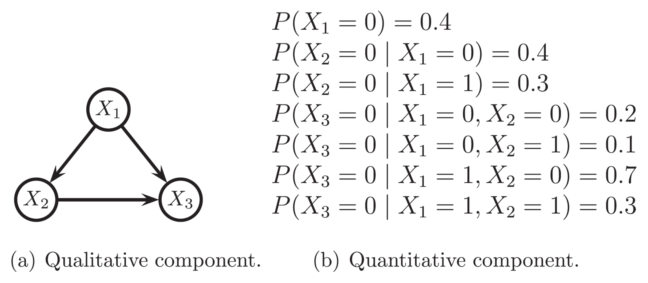
Bayesian networks (BN) are a statistical multivariate model for a set of variables . They have been developed for knowledge representation under uncertainty and can be defined in terms of two components:
BN were proposed for discrete variables. A broad and consolidated theory and methods can be found in the literature. However, environmental data often present continuous domains. In this case, the most common solution is to discretize the continuous variables and treat them as if they were discrete. Even though this does not always imply a wrong solution [35], it often can lead to a loss of precision. To avoid discretization, several approaches have been devised to represent probability distributions in hybrid domains (including continuous with/without discrete variables). The conditional Gaussian model is broadly used, but it imposes some restrictions that limit its applications to environmental data: (i) data must follow a multivariate Gaussian, and (ii) a discrete variable cannot have a continuous parent in the graph. These limitations have led to the development of other alternatives such as the Mixture of Truncated Exponential (MTEs) model, the Mixtures of Polynomials model, and the Mixtures of Truncated Basis Functions model (for more information, see [36,37,38,39]).
Discretization is often carried out by splitting the domain of the variable into several intervals and approximating the density function using a constant function. It can also be done by approximating the density function using a mixture of uniforms. However, if other functions are used, the accuracy of the approximation can be improved. One option is to use exponential functions to estimate the density functions and configure the so-called MTE model (for detailed information about MTE, see [40,41,42]). The advantage of MTEs is that they are closed under restriction, marginalization and combination, so standard BN inference processes can be applied. MTEs have been successfully used in environmental modeling [43,44].
BN also allow new information, or evidence, to be included in the model once it has been learnt, through the so-called inference process or probabilistic propagation. If we denote the set of evidence variables as , and their values as e, then the inference process consists of calculating the posterior distribution for each variable of interest in :
since is constant for all . Therefore, this process can be carried out by computing and normalizing the marginal probabilities in the following way:
where is the probability function obtained from replacing in the evidence variables by their values .
BN can cope with four different aims, depending on the number and nature of the target variable(s) [27]. When the focus is set on one target variable, we are dealing with regression (if it is continuous) or classification (when it is discrete).
In both regression and classification cases, the purpose is to predict the goal variable as precisely as possible, rather than trying to accurately model the joint probability of all the variables. For that reason, so-called fixed structures have been developed:
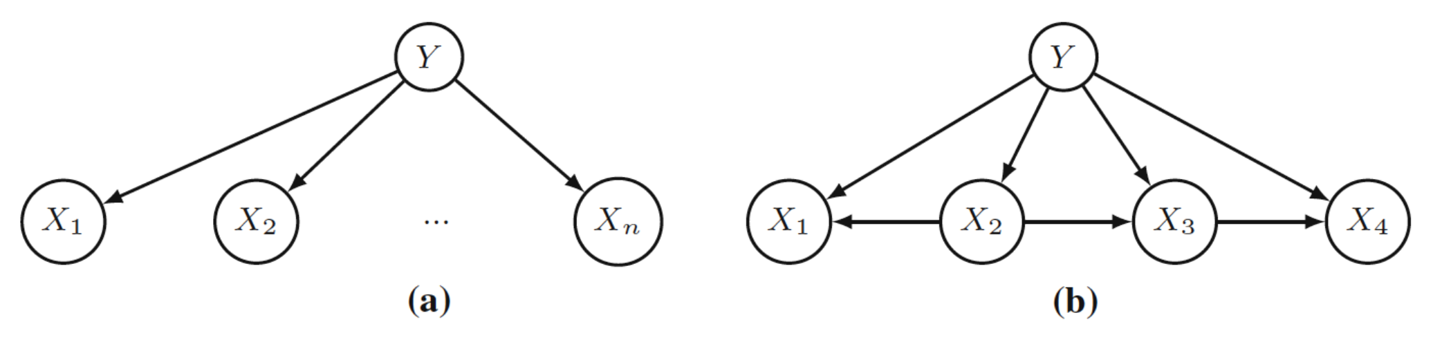
- Naïve Bayes (NB) [45] structure is a BN with a single root node and a set of feature variables with only the root node as a parent. Its name comes from the fact that the feature variables are independent given the root (Figure 2a). It is a naïve assumption that rarely holds in real problems, as feature variables may have direct dependencies.
- Tree-Augmented Naïve Bayes (TAN) [46] structure configures a step beyond NB, since each feature is allowed (but not forced) to have one more parent besides the target variable. This structure is first learnt as a directed tree structure with feature variables, using mutual information with respect to the target variable. In the second step, the relationships between the target variable and each feature are included (Figure 2b).
2.1. Regression Models Based on BN
Regression analysis consists of finding a model g that explains the target continuous variable Y in terms of a set of feature variables ; ...; , which can be discrete or continuous. Therefore, given a full observation of the features ; ...; , a prediction about Y can be obtained. The methodology applied to a regression model based on BN is explained in depth in [47].
A BN can be used as a regression model for prediction purposes if it contains a continuous response variable Y and a set of discrete and/or continuous feature variables ; ...; . Thus, to predict the value for Y from k observed features, the conditional density is computed, and a numerical prediction for Y is given using the expected value, as follows:
where represents the domain of Y.
Please note that is proportional to , and therefore, solving the regression problem would require a distribution to be specified over n variables given Y. The associated computational cost can be very high. However, using the factorization determined by the network, the cost is reduced. As we are interested in a model’s ability to simultaneously handle discrete and continuous variables without any restriction to the developed structure, the approach that best meets these requirements is the MTE model. Regarding inference, the posterior MTE distribution, , will be computed using the Variable Elimination algorithm [48,49,50].
To learn the model, we follow the approach of [51] to estimate the corresponding conditional distributions. Let and Y be two random variables, and consider the conditional density . The idea is to split the domain of Y using the equal frequency method with three intervals. Then, the domain of is also split using the properties of the exponential function, which is concave, and increases over its whole domain (see [42]). Accordingly, the partition consists of a series of intervals whose limits correspond to the points where empirical density changes between concavity and convexity, or decreases and increases. In case of models with more than one conditioning variable, see [52] for more details.
At this point, a five-parameter MTE is fitted for each split of the support of X, which means that in each split there will be five parameters to be estimated from data:
where and define the interval within which the density is estimated.
The reason to use the five-parameter MTE lies in its ability to fit the most common distributions accurately, while model complexity and the number of parameters to estimate is low [53]. The estimation procedure is based on least squares [42,54].
A natural way to obtain the predicted value from the distribution is to compute its expectation. Thus, the expected value of a random variable X with a density defined as in Equation (4) is computed as
If the density is defined by different intervals, the expected value would be the sum of the expression above for each part.
2.2. Classification Models Based on BN
When the response variable is discrete, we face a classification problem. If no information about the target (or class) variable is available, it is called an unsupervised classification or soft-clustering problem. This implies the partition of the data into groups in such a way that observations belonging to one group are similar to each other, but differ from observations in the other groups. Soft clustering based on BN allows the computation of the probability of each observation belonging to each group. This method has been previously applied to environmental problems. In this paper, we follow the methodology proposed by [55] and previously applied to socio-ecological management in [56,57]. The idea is to obtain a hidden variable with no previous information about its parameters or number of states, which reflects the different clusters considered. Therefore, the method consists of two steps (Figure 3):
- Estimation of the optimal number of states. Initially the class variable is considered to be a hidden variable, H, whose values are missing, because no information about it is given. The process starts by giving two states for the variable H, uniformly distributed (the same probability value for belonging to both groups). Now, the model is estimated based on an iterative procedure called the data augmentation method [58]: (a) the values of H are simulated for each observation according to the probability distribution of H, updated specifically for the corresponding observation, and (b) the parameters of the probability distribution are re-estimated according to newly simulated data. The BIC score of the model is computed in each iteration, and the process is repeated until there is no improvement. Thus, we have obtained the optimal parameters of the probability distribution function of the model in which the class variable has two states, and its likelihood value. The next step consists of a new iterative process in which a new state is included in variable H by splitting one of the existing states. The model is again re-estimated (by repeating the data augmentation method), and the BIC score is compared with the previous run. The process is repeated until there is no improvement in the BIC score, so the final model achieved will contain the optimal number of states.
- Computing the probability of each observation belonging to each group. Once we have obtained the final model, the next step consists of probability propagation, also called the inference process—for more information, see [41]. In this step, all the available information about the feature variables is input into the model as a new value called evidence, and propagated through the network, updating the probability distribution of the class variable, H. Finally, from this new distribution, the most probable state of the variable H for each data sample is achieved.
3. Case Study
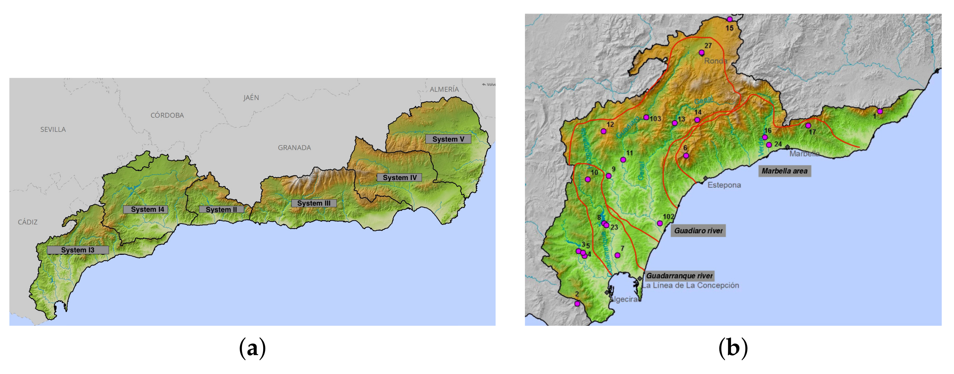
Mediterranean catchment areas in Andalusia (Figure 4a) comprise more than 17,000 km and 200 municipalities. The main characteristic is climatic variability, both in temperature and rainfall patterns, with deep differences between the humid west, with over 2000 mm annual rainfall (Systems I3 and I4) and the dry east, with less than 200 mm annual rainfall in some points of Almería (Systems IV and V). Both physical characteristics and relief make this area quite vulnerable to extreme climatic events. Flood, and especially flash flood, and abrupt relief cause intense events with several economic and, often, life costs. For example, in January 2021, a heavy storm event called Filomena caused more than 600 incidents in Andalusia, with 2 deaths and more than 200 L in 24 h. However, climate change predictions suggest a decrease in rainfall patterns in these areas, alongside an intensification of extreme events. This means less water, but over a shorter time and in an intense or even violent way.
Even when all systems (Figure 4a) are included in the Andalusian Mediterranean catchment areas, only System I3 presents the abovementioned data problems explained in depth in Section 3.1. Thus, this paper is focused on that system. This area can be divided into three parts—the Guadarranque river, Guadiaro river and Marbella area.
The Guadarranque river is located in Cádiz, in the region called Campo de Gibraltar, and belongs to the Alcornocales Natural Park. Its catchment area comprises 765 km and includes both the Guadarranque dam (with 87 hm of capacity) and a groundwater system. The Guadiaro river lies between Cádiz and Málaga and is the third longest river in the Andalusian. This catchment area comprises a total of 1504 km, including a set of natural areas with high ecological value. Its mean rainfall is one of the highest, with more than 700 hm per year. However, several human infrastructures have provoked blockage of its estuary, which increases flood risk and its negative consequences. Marbella presents one main river called the Río Verde, with one dam. This catchment area comprises more than 150 km. Moreover, this area includes a set of independent collection points that record rainfall data. Due to the important population settlement in this area, not only is the Río Verde modeled, but also information about rainfall around this area.
3.1. Data Collection and Preprocessing
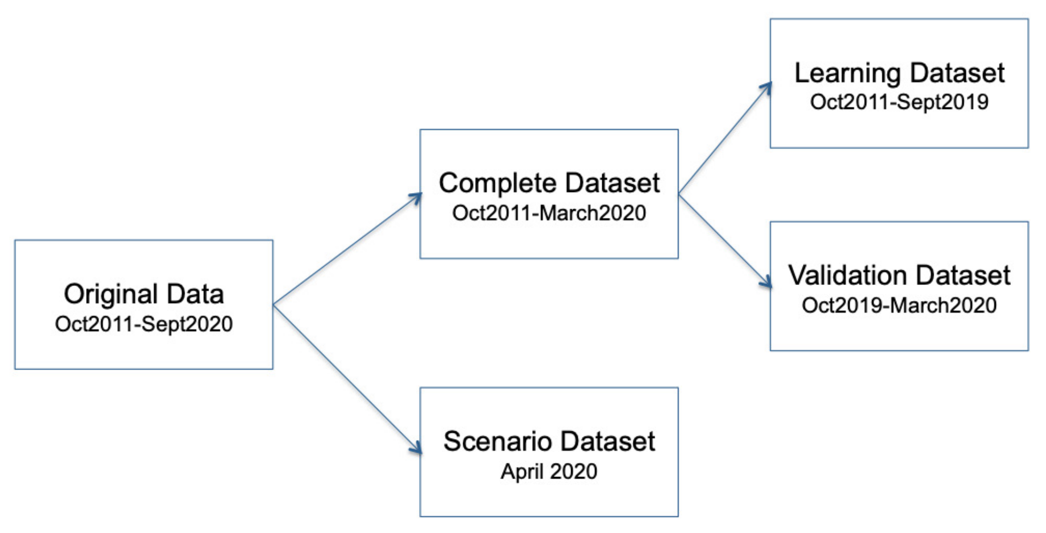
Data were collected from the Andalusia Hydrological Information System (SAIH, http://www.redhidrosurmedioambiente.es/saih accessed on 7 April 2022) and comprised a total of 73,636 observations over 25 continuous variables (Table 1 shows a summary of all variables). Complete hydrological years were used; thus, the months of October 2011 to September 2020 were included, with data obtained per hour.
Three datasets were created from the original—one per each area mentioned above. Their main characteristics are summarized in Table 2 and explained in depth in the sections below.
3.2. Missing Values: Guadarranque River
The Guadarranque dataset includes six continuous variables for rainfall and both dam or river level and volume. Variables for the dam missed observations from 1 May 2020 at 1:00 a.m. to September 2020, which means a total of 5 months and 3558 () missing values. The reason for this is unknown, but it is probably related to sensor damage. Due to mobility restrictions and lockdowns because of COVID-19, it may not have been repaired yet. To avoid removing these variables (dam level and volume) from the entire model, or even those missing months for all variables, a regression model based on BN is proposed as a modeling solution. The idea is to predict the values of dam level variable in such a way that we obtain a complete dataset with imputed values for missing data.
From the original dataset, the missing months (May to September 2020) were removed, and they are not used in this modeling step. Moreover, data for April 2020 were considered for validation purposes (Figure 5). In this way, a complete dataset is available for parameter estimation of the regression model. This was divided into learning and validation.
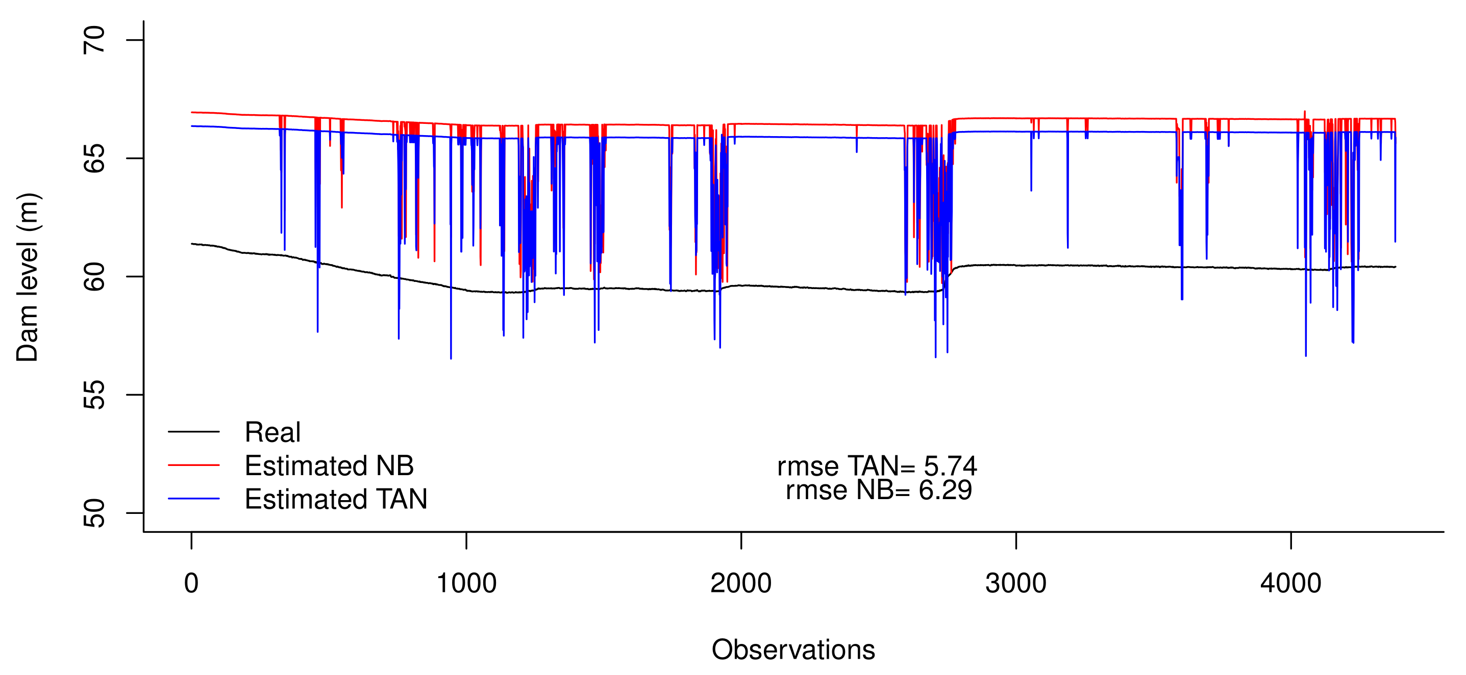
Regression models based on BN-fixed structures were developed in Elvira software [59] following the method explained in Section 2.1. Using the learning dataset, both NB and TAN models were learnt to check what fixed structure best fitted the data used for modeling. Thus, the response variable (dam level) would be modeled from the information provided by features (rainfall variables). In a second step, these models were validated using data from October 2019 to March 2020 (validation dataset)—see Figure 6a). The idea was to check if this methodology was able to accurately model the level variable. Validation was carried out using the inference process, including feature variable information as evidence, and computing the value for the response variable, dam level. As we have used a complete dataset, a comparison in terms of error rate can be made between real and predicted (imputed) values.
Once data imputation was carried out, we checked if this methodology and the use of imputed instead of real values could affect the final environmental conclusion. For this reason, an environmental problem was simulated in which the dam level variable needed to be modeled. In this case, the BN structure was not fixed, and was learnt using expert opinion, while parameter estimation was made using three different datasets (Figure 6b):
- Real data from October 2011 to March 2020;
- Imputed data with NB. Using the real dataset above, we considered the last six months were missing, and those values were imputed using the previously described NB model;
- Imputed data with TAN. In this case, six months with missing values were imputed using the TAN model, as previously described.
Finally, data from April 2020 was used as a scenario, and a comparison in terms of error rate was made between the model learnt with all real data versus those models learnt with six months of imputed data.
3.3. Lack of Information: Guadiaro River and Marbella Area
The lack of information problem appears in two of the areas—the Guadiaro river and Marbella. The Guadiaro dataset is the largest, with 14 variables. Rainfall variables present more than 94% of values equal to zero; therefore, they do not follow a standard distribution. This may imply inaccurate parameter estimation and a misleading inference process. For that reason, these variables were discretized. Several methods are available for data discretization. We chose to apply the equal frequency method [35] using Elvira software. This method divides data distribution in k bins intervals. The value of k is selected according to available data. It is true that if more bins were used, it would provide more information. However, it would also increase the granularity of the variables, and this implies more bins but fewer observations per bin, which could hinder the learning process. Thus, the selection for value k needs to have a balance between simplicity and informative power to reach effectiveness. According to expert knowledge, four bins was selected, in such a way that those values equaling zero belong to the first interval, and the rest of statistical information is divided into the other three intervals.
However, the problem is that no data about river level is collected in the lower part of the catchment area, which means no information about flood events is available. The coastal area is highly populated, and it is necessary to have this kind of information to acquire robust tools for flood management.
The Marbella dataset comprises five variables. Again, rainfall variables were discretized by equal frequency method into four intervals, while dam volume and level remained continuous. Unlike the Guadiaro river, Marbella does not present a unique riverbed, with all collected points associated with it. In this case, a set of hydrological stations is located surrounding the municipalities of Marbella and Estepona, both with high density population.
The solution proposed for this problem is unsupervised classification based on hybrid BN. This was performed according to the methodology explained in depth in Section 2.2. The algorithms were implemented in Elvira software, and NB structure was selected.
In this case, the feature variables were rainfall (discrete) and river and dam level (continuous). Through unsupervised classification, the class variable presented a set of groups with similar characteristics in terms of rainfall and river level. Thanks to the probabilistic nature of BN, not only can each observation be classified into one of the groups, but also its probability of belonging can be computed, which can give us further information. In this way, observations that could be classified in more than one group can be identified. Let us see an example of a class variable with three groups and a set of observations, whose probability of belonging to each group is shown in Table 3. Observations 1 and 4 are clearly classified into Groups 1 and 3, respectively. Additionally, Observation 2 presents the highest probability for Group 2, even when the value is lower. However, Observation 3 is equally likely to belong to Group 1 and 2. In this case, further analysis should be done.
4. Results and Discussion
In the previous section, two main problems were described that affect a total of three areas. In this section, the results are explained in each of the areas separately.
4.1. The Guadarranque River
The Guadarranque river area has % missing values for the dam level variable. In order to impute them, both NB and TAN regression models were developed. Using the learning dataset, model parameters were properly estimated. In a second step, the validation dataset was used in the following way: (i) each observation for feature variables was included as evidence, (ii) probabilistic propagation was carried out, and the density function for the target variable (dam level in this case) was obtained, and (iii) since we need a value for the variable, the most probable value was obtained from the distribution. This inference process was applied in both NB and TAN regression models.
Figure 7 shows a comparison between the real values for the validation dataset, and those imputed by NB and TAN. Error rate between real and imputed data were calculated, and their variance and mean bias error. Data imputed in both models can describe the general behavior of the real data; however, in both cases, values are overestimated. This is because only input information was taken into account (i.e., rainfall patterns) but not output (consumption rates, evapotranspiration, and other losses). Under the framework of SAICMA project, the idea is to model as accurately as possible the behavior of the Mediterranean catchment areas using as simple a model approach as possible. If we compare both regression models, TAN provides better results in terms of error rate. Its structure, including dependencies between feature variables, give more robustness to the predictions made.
Once data were imputed, our objective is to use the model for environmental purposes in the Guadarranque river area. Therefore, a Bayesian network model was developed with the aim of modeling dam behavior. The structure was learnt using expert knowledge, and it is shown in Figure 8. Parameter estimation was made using both real data and those datasets with data imputed from NB and TAN regression models. For each observation, models return the most probable value for dam level and a comparison between the predicted value and the value included in the dataset was made in terms of error rate (Table 4). Results show that in terms of error rate, there are no significant differences among the three models. However, variance shows lower values for the TAN structure.
4.2. The Guadiaro River
In this area, information about all collected points is available, but the lower area of the river does not have any data points. Despite the lack of information, we would like to acquire a model able to predict the risk of flood in this area, taking into account the behavior of the upper river area. For that purpose, unsupervised classification or clustering based on BN was carried out.
In this way, all data available (collected in the upper area) was used to establish a set of groups. Initially, the applied algorithm identified a total of five states for the hidden class variable as the optimal number of states. When these results are studied in detail, three states were set as the optimal results, since the fourth and fifth groups just included one or two observations. This is explained by the fact that these observations correspond to outliers for rainfall variables, i.e., a really extreme event. For that reason, they were included into Cluster 2.
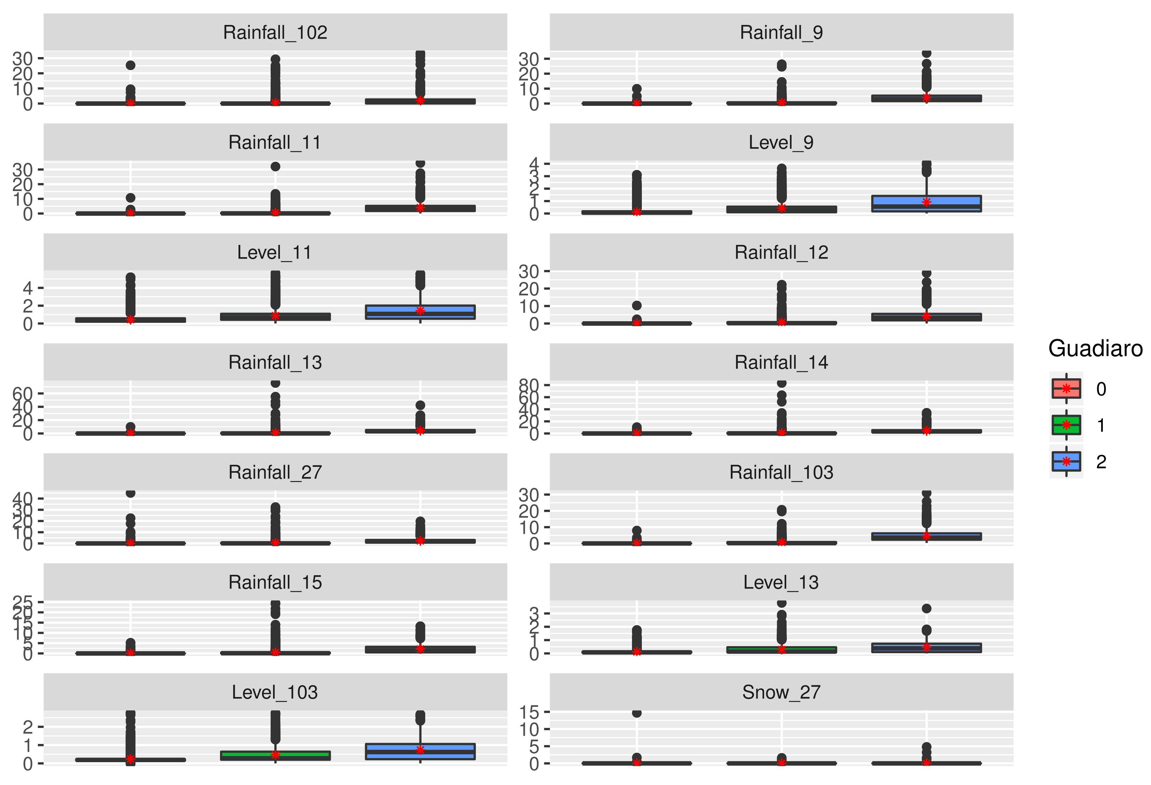
Therefore, a total of three groups or clusters (Figure 9) was identified and described below:
- Cluster 0. This sector (or cluster) includes most of the observations (Table 5). Rainfall variables are really low, with values around 0, which implies river variables also keep low levels. This cluster could be called a “dry situation” or even “normal situation”. Even when this area comprises one of the highest rainfall values, it is in a Mediterranean area, characterized by a long period of dry conditions with a set of short, humid periods.
- Cluster 1. With 7% of data (Table 5), rainfall variables present higher values than the previous cluster, with an important number of outliers. This is more evident in points located in the upper area (data-collection points 13, 14, 27 and 15). This suggests river levels increase their ranges and mean values (marked with a red point). As explained before, the Mediterranean area often presents storm events that feed riverbeds. In this case, the majority of rainfall lies in the upper areas of the mountain and flows down all the riverbeds, increasing its level. However, this kind of storm very often does not imply really dangerous consequences, since the reached values do not overcome the security threshold of the river. Therefore, this group or cluster could be entitled “storm situation”.
- Cluster 2. Finally, with 2% of the observations, all rainfall variables reach really high values, mainly those collected from points located in the middle of the river area (points 9, 11, 12 and 103). These are situated on the low side of the mountains, where storms coming from the Mediterranean and Atlantic seas are retained. In these cases, storms are shorter in time, but with higher volumes of rainfall, which can be observed in Figure 9. In this situation, river levels rise, reaching the highest values in comparison with other clusters. This could be called “extreme situation”.
4.3. The Marbella Area
The Marbella area is the smallest catchment and presents a set of independent rivers. Moreover, point 16, located in the Rio Verde, corresponds to a dam. In this area, there is an important human settlement that mainly depends on touristic activity related to the coastal area. Therefore, flood implies not only potential damage to infrastructures but also indirectly to the main economic activity, with the destruction of coastal areas.
Information collected from this area comprises a set of three points with a total of five variables, two of which are related to the dam. Again, unsupervised classification was carried out to classify the observation in a set of groups with similar characteristics.
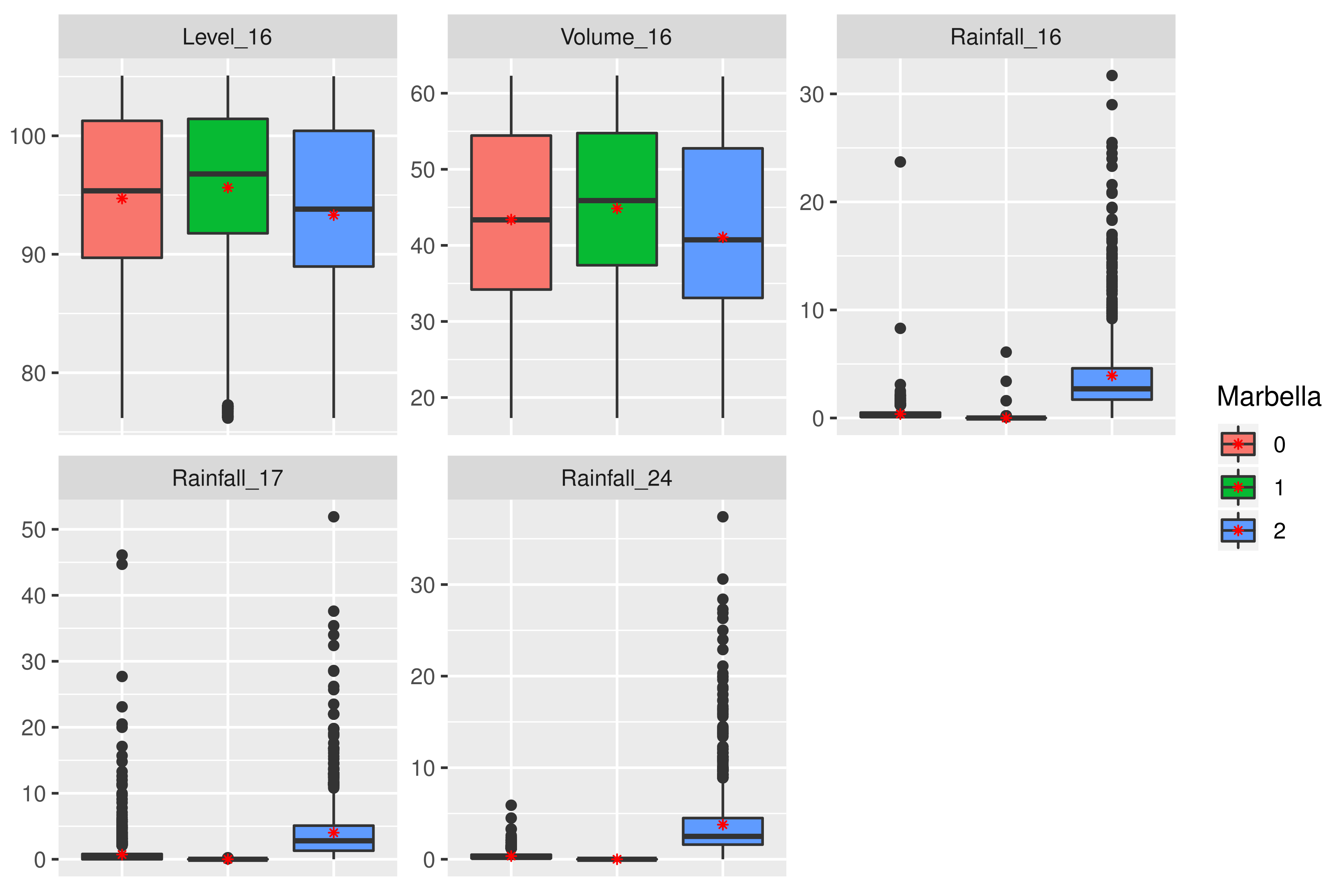
In this case, the optimal number of states is three, and box plots for the variables are shown in Figure 10. For dam variables, there are no significant differences among the three clusters, except for the case of rainfall. In Mediterranean areas, apart from a water supply function, dams also help keep the flood risk low, with the river flow under control. During a storm, the dam acts as a barrier that retains the increase of river level and releases the water flow at a controlled level.
In the case of rainfall variables, there are clear differences between the three clusters:
- Cluster 0. Even when values are low, they represent short events of rainfall with mean values around 0.3–0.5 mm. Therefore, this group could be called “drizzle situation”.
- Cluster 1. In this case, rainfall is equal to zero, with just some higher values in the case of point 16 (located in the dam). Therefore, this group could be called “dry situation”, which comprises % of the data (Table 6).
- Cluster 2. This cluster presents a clear difference with respect to the others, with rainfall values very high with mean values between 3 and 5 mm. Additionally, some outliers reach 30 or even 50 mm. This group is related to “extreme storm situation”. This cluster comprises % of the data.
5. Conclusions
Data preprocessing is the first and probably the most important step in a modeling process. Quality and quantity of data can determine the final model’s reliability. Data from the Andalusia Hydrological Information System were collected with the idea of creating a flood alert system. However, data present two issues: (i) missing values for one variable for a total of five months, and (ii) lack of information about river level in the coastal area. Both problems imply difficulties with the future modeling process. It is usual that real-life applications deal with imperfect data. Methods proposed in this paper aim to deal with this situation and allow data to be used in the best possible way.
Missing values have been extensively studied in the available literature, with several methods proposed. The difference with respect to our problem is the fact that missing values are commonly distributed along the dataset (independently they are random or not). In our case, however, missing information comprises a total of five complete months, which means close to the 5% of data. In these cases, the developed methods cannot deal with this problem. This is the main reason we are not performing a comparison with other techniques. However, an extensive comparison between BN and other regression methodologies can be found in [47]. Thus, in this paper we proposed a solution consisting of applying a data imputation method based on the BN regression model. It is true that the applied models overestimate the results, since no information about the outcomes of the dam are available (consumption rates, evaporation rates, etc. In comparisons, the best results are provided by the TAN structure in terms of error rate and variance. Its structure, including dependencies between feature variables, gives more robustness to the given predictions, in comparison with NB. Additionally, despite the overestimation, results for the imputed data show that there are no significant differences between the model learnt with real and imputed data. This means that regression based on BN-fixed structures is a powerful tool for data imputation, since it can predict those missing values.
The second problem is related to the lack of information, because of the non-existence of a river level sensor in the lower part of the river. In this case, the solution proposed is based on so-called soft clustering or unsupervised classification using BN. This was applied to two different areas and three groups were obtained: (1) dry situation, with no rainfall, (2) low rainfall event, and (3) extreme event. Following this methodology, the probability of belonging to each group is also provided. It means that when new information is included (for example, rainfall predictions), the model is able to provide the probability of being a dry, normal or extreme event situation in advance.
This paper applies the traditional BN models to overcome a set of data-collection problems. The novelty of this approach lies not in the methodology itself, but in how it can be applied to a real-life problem. The use of this well-known, and therefore, well-tested methodology to a real data problem could help stakeholders and experts avoid the removal or rejecting of a dataset just because of a lack of information or partially unavailable values. Thus, the solutions proposed help to overcome two deep problems found in the initial step of a research project. For a future work, imputed data for the missing values problem will be used for modeling flood risk in the study area. On the other hand, unsupervised classification models will be used in scenarios of real storm events, with the aim of checking their efficiency of predicting a flood situation.
Author Contributions
R.F.R. developed the models, M.J.F. performed the results analysis, and R.R. supervised the study and wrote the methodological part of the paper. All authors read and agreed to the published version of the manuscript.
Funding
This research was funded by Regional Government of Andalusia of grant number: UAL18-TIC-A011-B-E, Ministry of Economy, Industry and Competitiveness of grant number: PID2019-106758GB-C32/AEI/10.13039/501100011033 and Ministry of Economy, Industry and Competitiveness of grant number: PID2019-106758GB-C33/AEI/10.13039/501100011033.
Institutional Review Board Statement
Not applicable.
Informed Consent Statement
Not applicable.
Data Availability Statement
Not applicable.
Conflicts of Interest
The authors declare no conflict of interest.
References
- Marhavilas, P.; Koulouriotis, D.; Gemeni, V. Risk analysis and assessment methodologies in the work sites: On a review, classification and comparative study of the scientific literature of the period 2000–2009. J. Loss Prev. Process Ind. 2011, 24, 477–523. [Google Scholar] [CrossRef]
- Apel, H.; Aronica, G.; Kreibich, H.; Thieken, A. Flood risk analyses-how detailed do we need to be? Nat. Hazards 2009, 49, 79–98. [Google Scholar] [CrossRef]
- Jonkmand, S.; Bockarjova, M.; Kok, M.; Bernardini, P. Integrated hydrodynamic and economic modelling of flood damage in the Netherlands. Ecol. Econ. 2008, 66, 77–90. [Google Scholar] [CrossRef]
- Kaikkonen, L.; Tuuli, P.; Rahikainen, M.; Uusitalo, L.; Lehikoinen, A. Bayesian Networks in Environmental Risk Assessmen: A review. Integr. Environ. Assess. Manag. 2021, 17, 62–78. [Google Scholar] [CrossRef] [PubMed]
- Lavender, L.K. Plastics in the Marine Environment. Mar. Sci. 2017, 9, 205–229. [Google Scholar]
- McDermott, T.; Surminski, S. How normative interpretations of climate risk assessment affect local decision-making: An exploratory study at the city scale in Cork, Ireland. Philos. Trans. A 2018, 376, 20170300. [Google Scholar] [CrossRef] [Green Version]
- Kuklicke, C.; Demeritt, D. Adaptative and risk-based approaches to climate change and the management of uncertainty and institutional risk: The case of future flooding in Engiand. Glob. Environ. Chang. 2016, 37, 56–68. [Google Scholar] [CrossRef] [Green Version]
- Hodgson, E.E.; Essington, T.E.; Samhouri, J.; Allison, E.; Bennett, N.; Bostrom, A.; Cullen, A.; Kasperski, S.; Levin, P.; Poe, M. Integrated Risk Assessment for the Blue Economy. Front. Mar. Sci. 2019, 6, 1–14. [Google Scholar] [CrossRef]
- Morss, R.E.; Wilhelmi, O.; Downton, M.; Gruntfest, E. Flood risk, uncerttainty, and scientific information for decision making. Lessons from an interdisciplinary project. Am. Meteorol. Soc. 2005, 1593–1601. [Google Scholar] [CrossRef]
- Caballero-Gallardo, K.; Alcala-Orozco, M.; Barraza-Quiroz, D.; la Rosa, J.D.; Olivero-Verbel, J. Environmental risks associated with trace elements in sediments from Cartagena Bay, an industrialized site at the Caribbean. Chemosphere 2020, 242, 1–12. [Google Scholar] [CrossRef]
- CEA. Reducing the Social and Economic Impact of Climate Change and Natural Catastrophes: Insurance Solutions and Public-Private Partnerships; Technical Report; European Insurance and Reinsurance Federation: Brussels, Belgium, 2007. [Google Scholar]
- Kundzewicz, Z.; Krysanova, V.; Dankers, R.; Hirabayashi, Y.; Kanae, S.; Hattermann, F.; Huang, S.; Milly, P.; Stoffel, M.; Driessen, P.; et al. Differences in flood hazard projections in Europe - their causes and consequences for decision making. Hydrol. Sci. J. 2017, 62, 1–14. [Google Scholar] [CrossRef] [Green Version]
- Bertola, M.; Viglione, A.; Vorogushyn, S.; Lun, D.; Merz, B.; Bloschl, G. Do small and large floods have the same drivers of change? A regional attribution analysis in Europe. Hydrol. Earth Syst. Sci. 2021, 25, 1347–1364. [Google Scholar] [CrossRef]
- Arnell, N.; Gosling, S. The impacts of climate change on river flood risk at the global scale. Clim. Chang. 2016, 134, 387–401. [Google Scholar] [CrossRef] [Green Version]
- Nicholls, R.J.; Hoozemans, F.M.; Marchand, M. Increasing flood risk and wetland losses due to global sea-level rise: Regional and global analyses. Glob. Environ. Chang. 1999, 9, 69–87. [Google Scholar] [CrossRef]
- Moel, H.; Aerts, J. Effect of uncertainty in land use, damage models and inundation depth on flood damage estimates. Nat. Hazards 2011, 58, 407–425. [Google Scholar] [CrossRef] [Green Version]
- Moel, H.; van Alphen, J.; Aerts, J. Flood maps in Europe-methods, availability and use. Nat. Hazards Earth Syst. Sci. 2009, 9, 289–301. [Google Scholar] [CrossRef] [Green Version]
- Masuda, M.M.; Sackorb, A.S.; Alamc, A.F.; Al-Amind, A.Q.; Ghanif, A.B.A. Community responses to flood risk management—An empirical Investigation of the Marine Protected Areas (MPAs) in Malaysia. Mar. Policy 2018, 97, 119–126. [Google Scholar] [CrossRef]
- Sairam, N.; Schroter, K.; Ludtke, S.; Merz, B.; Kreibich, H. Quantifying Flood Vulnerability Reduction via Private Precaution. Earth’s Future 2019, 7, 235–249. [Google Scholar] [CrossRef]
- Lechowska, E. What determines flood risk perception? A review of factors of flood risk perception and relations between its basic elements. Nat. Hazards 2018, 94, 1341–1366. [Google Scholar] [CrossRef] [Green Version]
- Alfieri, L.; Feyen, L.; Dottori, F.; Bianchi, A. Ensemble flood risk assessment in Europe under high end climate scenarios. Glob. Environ. Chang. 2015, 35, 199–212. [Google Scholar] [CrossRef]
- Guhathakurta, P.; Sreejith, O.; Menon, P. Impact of climate change on extreme rainfall events and flood risk in India. J. Earth Syst. Sci. 2011, 120, 359–373. [Google Scholar] [CrossRef]
- Lyu, H.; Sun, W.; Shen, S.; Arulrajah, A. Flood risk assessment in metro systems of mega-cities using a GIS-based modelling approach. Sci. Total Environ. 2018, 626, 1012–1025. [Google Scholar] [CrossRef] [PubMed]
- Guillen, J.D.H.; del Rey, A.M.; Casado-Vara, R. Propagation of the Malware Used in APTs Based on Dynamic Bayesian Networks. Mathematics 2021, 9, 3097. [Google Scholar]
- Maldonado, A.D.; Morales, M.; Navarro, F.; Sánchez-Martos, F.; Aguilera, P.A. Modeling Semiarid River–Aquifer Systems with Bayesian Networks and Artificial Neural Networks. Mathematics 2022, 10, 107. [Google Scholar] [CrossRef]
- Rodríguez-Martínez, A.; Vitoriano, B. Probability-BasedWildfire Risk Measure for Decision-Making. Mathematics 2020, 8, 557. [Google Scholar] [CrossRef]
- Aguilera, P.A.; Fernández, A.; Fernández, R.; Rumí, R.; Salmerón, A. Bayesian networks in environmental modelling. Environ. Model. Softw. 2011, 26, 1376–1388. [Google Scholar] [CrossRef]
- Niazi, M.; Morales Nápoles, O.; vanWesenbeeck, B. Probabilistic Characterization of the Vegetated Hydrodynamic System using Non-Parametric Bayesian Networks. Water 2021, 13, 398. [Google Scholar] [CrossRef]
- Paprotny, D.; Kreibich, H.; Morales-Nápoles, O.; Wagenaar, D.; Castellarin, A.; Carisi, F.; Bertin, X.; Merz, B.; Schroter, K. A probabilistic approach to estimating residential losses from different flood types. Nat. Hazards 2021, 105, 2569–2601. [Google Scholar] [CrossRef]
- Wu, Z.; Shen, Y.; Wang, H.; Wu, M. Urban flood disaster risk evaluation based on ontology and Bayesian Network. J. Hydrol. 2020, 583, 1–15. [Google Scholar] [CrossRef]
- Paprotny, D.; Morales-Nápoles, O. Estimating extreme river discharges in Europe through a Bayesian network. Hydrol. Earth Syst. Sci. 2017, 21, 2615–2636. [Google Scholar] [CrossRef] [Green Version]
- Yuji, R.; Heo, G.; Whang, S.E. A survey on data collection for machine learning: A big data- AI intregration perspective. IEEE Trans. Knowl. Data Eng. 2021, 33, 1328–1347. [Google Scholar]
- Lecomte, J.; Benoit, H.; Etienne, M.; Bel, L.; Parent, E. Modeling the habitat associations and spatial distribution of benthic macroinvertebrates: A hierarchical Bayesian model for zero-inflated biomass data. Ecol. Model. 2013, 265, 74–84. [Google Scholar] [CrossRef]
- Maldonado, A.; Aguilera, P.A.; Salmerón, A.; José-Miguel Sánchez-Pérez, A.R.E. (Eds.) An Experimental Comparison of Methods to Handle Missing Values in Environmental Datasets. In Proceedings of the International Environmental Modelling and Software Society (iEMSs) 8th International Congress on Environmental Modelling and Software, Toulouse, France, 10–14 July 2016. [Google Scholar]
- Ropero, R.F.; Renooij, S.; van der Gaag, L. Discretizing environmental data for learning Bayesian-network classifiers. Ecol. Model. 2018, 368, 391–403. [Google Scholar] [CrossRef]
- Langseth, H.; Nielsen, T.D.; Rumí, R.; Salmerón, A. Mixtures of Truncated Basis Functions. Int. J. Approx. Reason. 2012, 53, 212–227. [Google Scholar] [CrossRef] [Green Version]
- Shenoy, P.P.; West, J.C. Inference in hybrid Bayesian networks using mixtures of polynomials. Int. J. Approx. Reason. 2011, 52, 641–657. [Google Scholar] [CrossRef] [Green Version]
- Rumí, R. Modelos de Redes Bayesianas con Variables Discretas y Continuas. Ph.D. Thesis, Universidad de Almería, Almería, Spain, 2003. [Google Scholar]
- Moral, S.; Rumí, R.; Salmerón, A. Mixtures of Truncated Exponentials in Hybrid Bayesian Networks. In Lecture Notes in Artificial Intelligence, Proceedings of the ECSQARU’01, Toulouse, France, 19–21 September 2001; Springer: Berlin/Heidelberg, Germany, 2001; Volume 2143, pp. 156–167. [Google Scholar]
- Cobb, B.R.; Rumí, R.; Salmerón, A. Bayesian Networks Models with Discrete and Continuous Variables. In Advances in Probabilistic Graphical Models; Studies in Fuzziness and Soft Computing; Springer: Berlin/Heidelberg, Germany, 2007; pp. 81–102. [Google Scholar]
- Rumí, R.; Salmerón, A. Approximate probability propagation with mixtures of truncated exponentials. Int. J. Approx. Reason. 2007, 45, 191–210. [Google Scholar] [CrossRef] [Green Version]
- Rumí, R.; Salmerón, A.; Moral, S. Estimating mixtures of truncated exponentials in hybrid Bayesian networks. Test 2006, 15, 397–421. [Google Scholar] [CrossRef]
- Flores, J.; Ropero, R.F.; Rumí, R. Assessment of flood risk in Mediterranean catchments: An approach based on Bayesian networks. Stoch. Environ. Res. Risk Assess. 2019, 33, 1991–2005. [Google Scholar] [CrossRef]
- Maldonado, A.; Aguilera, P.; Salmerón, A. Continuous Bayesian networks for probabilistic environmental risk mapping. Stoch. Environ. Res. Risk Assess. 2016, 30, 1441–1455. [Google Scholar] [CrossRef]
- Minsky, M. Steps towards artificial intelligence. Comput. Thoughts 1961, Volume 49, 8–30. [Google Scholar] [CrossRef]
- Friedman, N.; Geiger, D.; Goldszmidt, M. Bayesian Network Classifiers. Mach. Learn. 1997, 29, 131–163. [Google Scholar] [CrossRef] [Green Version]
- Ropero, R.F.; Aguilera, P.A.; Fernández, A.; Rumí, R. Regression using hybrid Bayesian networks: Modelling landscape-socioeconomy relationships. Environ. Model. Softw. 2014, 57, 127–137. [Google Scholar] [CrossRef]
- Li, Z.; D’Ambrosio, B. Efficient inference in Bayes networks as a combinatorial optimization problem. Int. J. Approx. Reason. 1994, 11, 55–81. [Google Scholar] [CrossRef] [Green Version]
- Dechter, R. Bucket elimination: A unifying framework for probabilistic inference algorithms. In Proceedings of the Twelfth Conference on Uncertainty in Artificial Intelligence, Portland, OR, USA, 1–4 August 1996; pp. 211–219. [Google Scholar]
- Zhang, N.L.; Poole, D. Exploiting causal independence in Bayesian network inference. J. Artif. Intell. Res. 1996, 5, 301–328. [Google Scholar] [CrossRef] [Green Version]
- Morales, M.; Rodríguez, C.; Salmerón, A. Selective naïve Bayes for regression using mixtures of truncated exponentials. Int. J. Uncertain. Fuzziness Knowl. Based Syst. 2007, 15, 697–716. [Google Scholar] [CrossRef]
- Moral, S.; Rumí, R.; Salmerón, A. Approximating conditional MTE distributions by means of mixed trees. In Lecture Notes in Artificial Intelligence, Proceedings of the ECSQARU’03, Aalborg, Denmark, 2–5 July 2003; Springer: Berlin/Heidelberg, Germany, 2003; Volume 2711, pp. 173–183. [Google Scholar]
- Cobb, B.R.; Shenoy, P.P.; Rumí, R. Approximating Probability Density Functions with Mixtures of Truncated Exponentials. Stat. Comput. 2006, 16, 293–308. [Google Scholar] [CrossRef] [Green Version]
- Romero, V.; Rumí, R.; Salmerón, A. Learning hybrid Bayesian networks using mixtures of truncated exponentials. Int. J. Approx. Reason. 2006, 42, 54–68. [Google Scholar] [CrossRef] [Green Version]
- Fernández, A.; Gámez, J.A.; Rumí, R.; Salmerón, A. Data clustering using hidden variables in hybrid Bayesian networks. Prog. Artif. Intell. 2014, 2, 141–152. [Google Scholar] [CrossRef] [Green Version]
- Ropero, R.F.; Aguilera, P.A.; Rumí, R. Analysis of the socioecological structure and dynamics of the territory using a hybrid Bayesian network classifier. Ecol. Model. 2015, 311, 73–87. [Google Scholar] [CrossRef]
- Aguilera, P.A.; Fernández, A.; Ropero, R.F.; Molina, L. Groundwater quality assessment using data clustering based on hybrid Bayesian networks. Stoch. Environ. Res. Risk Assess. 2013, 27, 435–447. [Google Scholar] [CrossRef]
- Tanner, M.A.; Wong, W.H. The calculation of posterior distributions by data augmentation. J. Am. Stat. Assoc. 1987, 82, 528–550. [Google Scholar] [CrossRef]
- Elvira-Consortium. Elvira: An Environment for Creating and Using Probabilistic Graphical Models. In Proceedings of the First European Workshop on Probabilistic Graphical Models, Cuenca, Spain, 6–8 November 2002; pp. 222–230. [Google Scholar]
Figure 1.
A discrete Bayesian network with three binary variables.

Figure 2.
Naïve Bayes (NB) (a) and Tree-Augmented Naïve Bayes (TAN) (b) structures.

Figure 3.
Outline of the unsupervised classification based on hBN probabilistic clustering. Dotted lines represent the relationships between the variables when parameters have not been estimated yet. B, BIC score. Figure adapted from [56].
Figure 3.
Outline of the unsupervised classification based on hBN probabilistic clustering. Dotted lines represent the relationships between the variables when parameters have not been estimated yet. B, BIC score. Figure adapted from [56].

Figure 4.
Location of Mediterranean catchment areas (a) and System I3 (b). Points represent data-collecting stations. Maps obtained from SAIH website.
Figure 4.
Location of Mediterranean catchment areas (a) and System I3 (b). Points represent data-collecting stations. Maps obtained from SAIH website.

Figure 5.
Guadarranque data preprocessing.

Figure 6.
Outline of the Guadarranque regression models for missing value imputation (a) and environmental scenario evaluation (b).
Figure 6.
Outline of the Guadarranque regression models for missing value imputation (a) and environmental scenario evaluation (b).

Figure 7.
Real values for dam level variable and those imputed by NB and TAN regression models.

Figure 8.
Structure of the Bayesian network model learnt for the Guadarranque river area. Elvira software was used for both model-learning and posterior parameter estimation.
Figure 8.
Structure of the Bayesian network model learnt for the Guadarranque river area. Elvira software was used for both model-learning and posterior parameter estimation.

Figure 9.
Box plots of the cluster identified for the Guadiaro river through unsupervised classification. Each graph represents a box plot in the three clusters for each variable. Variable names correspond to their codes in the dataset and collected point. Red point marks the mean.
Figure 9.
Box plots of the cluster identified for the Guadiaro river through unsupervised classification. Each graph represents a box plot in the three clusters for each variable. Variable names correspond to their codes in the dataset and collected point. Red point marks the mean.

Figure 10.
Box plots of the cluster identified for the Marbella area through unsupervised classification. Each graph represents the box plot in the three clusters for each variable. Variable names correspond to their codes in the dataset and collected point. Red point marks the mean.
Figure 10.
Box plots of the cluster identified for the Marbella area through unsupervised classification. Each graph represents the box plot in the three clusters for each variable. Variable names correspond to their codes in the dataset and collected point. Red point marks the mean.


Table 1.
Summary of the variables collected.
| Area | Variable | Min | 1st Qu | Mean | 3rd Qu | Max |
|---|---|---|---|---|---|---|
| Marbella | Level 16 | 76.18 | 91.66 | 95.56 | 101.42 | 105.09 |
| Volume 16 | 17.31 | 37.21 | 44.75 | 54.74 | 62.33 | |
| Rainfall 16 | 0 | 0 | 0.07108 | 0 | 31.7 | |
| Rainfall 17 | 0 | 0 | 0.08334 | 0 | 51.9 | |
| Rainfall 24 | 0 | 0 | 0.06778 | 0 | 37.4 | |
| Guadiaro | Rainfall 102 | 0 | 0 | 0.05783 | 0 | 33.4 |
| Rainfall 9 | 0 | 0 | 0.09427 | 0 | 33.8 | |
| Rainfall 11 | 0 | 0 | 0.09039 | 0 | 34.4 | |
| Level 9 | 0 | 0.01 | 0.1548 | 0.2 | 4.06 | |
| Level 11 | 0 | 0.21 | 0.47 | 0.62 | 5.67 | |
| Rainfall 12 | 0 | 0 | 0.1086 | 0 | 28.9 | |
| Rainfall 13 | 0 | 0 | 0.1042 | 0 | 75.7 | |
| Rainfall 14 | 0 | 0 | 0.1197 | 0 | 83.5 | |
| Rainfall 27 | 0 | 0 | 0.07038 | 0 | 45 | |
| Rainfall 103 | 0 | 0 | 0.1123 | 0 | 31 | |
| Rainfall 15 | 0 | 0 | 0.0663 | 0 | 24.6 | |
| Level 13 | 0 | 0.05 | 0.1328 | 0.14 | 3.79 | |
| Level 103 | 0 | 0.15 | 0.263 | 0.25 | 2.76 | |
| Snow 27 | 0 | 0 | 4.70 × 10 | 0 | 14.7 | |
| Guadarranque | Level 8 | 50.84 | 60.98 | 65.7 | 69.57 | 73.39 |
| Volume 8 | 17.59 | 45.2 | 61.28 | 73.86 | 88.97 | |
| Rainfall 23 | 0 | 0 | 0.087 | 0 | 55.6 | |
| Rainfall 8 | 0 | 0 | 0.08665 | 0 | 40.5 | |
| Rainfall 10 | 0 | 0 | 0.1151 | 0 | 34.7 |
Table 2.
Dataset characteristics, number of variables (#Var.), types (C, continuous or H, hybrid) and number of rainfall, level or snow variables. * Discretized variables.
Table 2.
Dataset characteristics, number of variables (#Var.), types (C, continuous or H, hybrid) and number of rainfall, level or snow variables. * Discretized variables.
| Dataset | #Var. | Type | Rainfall | Level/Vol. | Snow |
|---|---|---|---|---|---|
| Guadarranque | 6 | C | 4 | 2 | 0 |
| Guadiaro | 14 | H | 9 * | 4 | 1 * |
| Marbella | 5 | H | 3 * | 2 | 0 |
| Total | 25 | - | 16 | 8 | 1 |
Table 3.
Example of a set of observations and their probability of belonging to each group.
| Observation | Group 1 | Group 2 | Group 3 |
|---|---|---|---|
| 1 | 0.9 | 0.05 | 0.05 |
| 2 | 0.1 | 0.6 | 0.3 |
| 3 | 0.4 | 0.4 | 0.2 |
| 4 | 0.05 | 0.01 | 0.94 |
Table 4.
Error rate, variance and mean bias error for the Bayesian network model for the Guadarranque river. MBE—Mean Bias Error.
Table 4.
Error rate, variance and mean bias error for the Bayesian network model for the Guadarranque river. MBE—Mean Bias Error.
| Model | rmse | Variance | MBE |
|---|---|---|---|
| Real | |||
| NB Imputed | |||
| TAN Imputed |
Table 5.
Observations per each cluster in Guadiaro river.
| Cluster | Observations | % |
|---|---|---|
| Dry situation (0) | 69,710 | 91 |
| Storm situation (1) | 5558 | 7 |
| Extreme situation (2) | 1094 | 2 |
Table 6.
Observations per each cluster in Marbella area.
| Cluster | Observations | % |
|---|---|---|
| Drizzle situation (0) | 2294 | 3 |
| Dry situation (1) | 72,909 | |
| Extreme storm situation (2) | 1159 |
Publisher’s Note: MDPI stays neutral with regard to jurisdictional claims in published maps and institutional affiliations. |
© 2022 by the authors. Licensee MDPI, Basel, Switzerland. This article is an open access article distributed under the terms and conditions of the Creative Commons Attribution (CC BY) license (https://creativecommons.org/licenses/by/4.0/).
Share and Cite
MDPI and ACS Style
Ropero, R.F.; Flores, M.J.; Rumí, R. Bayesian Networks for Preprocessing Water Management Data. Mathematics 2022, 10, 1777. https://0-doi-org.brum.beds.ac.uk/10.3390/math10101777
AMA Style
Ropero RF, Flores MJ, Rumí R. Bayesian Networks for Preprocessing Water Management Data. Mathematics. 2022; 10(10):1777. https://0-doi-org.brum.beds.ac.uk/10.3390/math10101777
Chicago/Turabian StyleRopero, Rosa Fernández, María Julia Flores, and Rafael Rumí. 2022. "Bayesian Networks for Preprocessing Water Management Data" Mathematics 10, no. 10: 1777. https://0-doi-org.brum.beds.ac.uk/10.3390/math10101777
Note that from the first issue of 2016, this journal uses article numbers instead of page numbers. See further details here.