Application of HMM and Ensemble Learning in Intelligent Tunneling

Abstract

The cutterhead torque and thrust, reflecting the obstruction degree of the geological environment and the behavior of excavation, are the key operating parameters for the tunneling of tunnel boring machines (TBMs). In this paper, a hybrid hidden Markov model (HMM) combined with ensemble learning is proposed to predict the value intervals of the cutterhead torque and thrust based on the historical tunneling data. First, the target variables are encoded into discrete states by means of HMM. Then, ensemble learning models including AdaBoost, random forest (RF), and extreme random tree (ERT) are employed to predict the discrete states. On this basis, the performances of those models are compared under different forms of the same input parameters. Moreover, to further validate the effectiveness and superiority of the proposed method, two excavation datasets including Beijing and Zhengzhou from the actual project under different geological conditions are utilized for comparison. The results show that the ERT outperforms the other models and the corresponding prediction accuracies are up to 0.93 and 0.99 for the cutterhead torque and thrust, respectively. Therefore, the ERT combined with HMM can be used as a valuable prediction tool for predicting the cutterhead torque and thrust, which is of positive significance to alert the operator to judge whether the excavation is normal and assist the intelligent tunneling.

1. Introduction

Due to the advantages of higher efficiency, safety and environmental friendliness, tunnel boring machines (TBMs) have been increasingly used in water conservancy, highway and railway tunnel construction [1]. Once the special situation occurs or the operation is not timely for the TBMs, it may cause jamming, collapse, and other serious consequences. Therefore, the reasonable setting of TBM tunneling parameters is of vital significance to ensure tunneling security and efficiency. However, caused by complex geological conditions and numerous operating parameters, the prediction of key parameters of TBM is still challenging and has attracted the attention of many researchers. In practical tunnel construction, cutterhead torque and total thrust are the important operational parameters of TBMs, reflecting the obstruction degree of geological conditions and excavation behavior [2]. There are many important works reported in recent decades. The methods for predicting the operational parameters can be typically categorized into two classes: physical model methods (combined with experiments) and data-driven methods (machine learning and deep learning).

Physical model methods mainly include empirical model methods, rock–soil mechanics analysis methods, and numerical simulation methods. Krause [3] given the first empirical formula for calculating cutter torque and thrust, which has been widely used by designers of related enterprise. The quantitative relationship between cutterhead torque and other design parameters was established under different geological conditions by Ates et al. [4]. Zhang et al. [5] analyzed the influences of geological and operating parameters, and they proposed an approximate calculation method for the thrust and torque. The methodology to calculate thrust and torque was presented in the mixed-face ground [6]. Faramarzi et al. [7] established prediction models to estimate the torque and thrust by utilizing the discrete element method.

Those physical methods mentioned above give insights into the prediction of the cutterhead torque, which provides certain guidances for TBM design in practice. However, there are still obvious limits in practical applications because those methods commonly require prior knowledge of geological parameters and system parameters. With the advancement of data-driven techniques, physical methods were widely used in earlier research, but now, data-driven methods are more popular.

For data-driven methods, Sun et al. [8] established a load prediction model for TBMs by using random forest (RF) to predict the operational parameters such as cutterhead torque and thrust based on the geological data and operational parameters. Subsequently, they employed three different recurrent neural network (RNN) models including traditional RNNs, long-short term memory (LSTM), and gated recurrent unit (GRU) to predict the TBM operation parameters in real time [9]. Song et al. [10] used a novel fuzzy c-means clustering-based time series segmentation method to segment operation parameter sequences, and they further used support vector machine regression (SVR) to predict the cutterhead thrust. Leng et al. [11] proposed a hybrid data-mining approach to process the real-time monitoring data from TBM automatically. Using the change point detection method based on linear regression, Hong et al. [12] segmented operation parameter sequences and established the separate prediction models for the cutter torque at each stage. Qin et al. [13] presented a novel hybrid deep neural network (HDNN) for accurately predicting the cutterhead torque for shield tunneling machines based on the equipment operational and status parameters. A novel adaptive residual long short-term network was presented to predict cutterhead torque across domains under changeable geological conditions [14]. Xu et al. [15] established prediction methods for rotation speed, advance rate, and torque by comparing the different machine learning methods and deep neural networks.

It is seen that those data-driven methods have outperformed the physical models for the prediction of key operational parameters of TBM, but there are still some limitations. On the one hand, we noticed that the sampling period of data collection in the data acquisition system is usually 5 s, so the operating parameters fluctuate rapidly with 5 s intervals. If the specific predicted values are returned in real time with 5 s intervals, the values jump frequently, which will not assist the shield driver in adjusting the operating parameters as a guide. The main purpose of this paper is not simply to propose a prediction method but is aimed to assist the driver in the actual tunneling process. A large number of input parameters are needed in the above data-driven methods, so even if the real-time cutterhead torque is predicted, the operator cannot adjust the panel parameters to match the cutterhead torque in time, which may make some disturbance to the operators. On the other hand, for the deep learning algorithms, gradient disappearance and model degradation will occur as the number of layers increases, as well as the computational complexity will be large.

To solve the above-mentioned problems and better apply prediction models to assist intelligent tunneling, a novel hybrid prediction model combining Hidden Markov Model (HMM) and ensemble learning is proposed for the prediction of key parameters of TBM. The objective of this paper is to predict the interval of values rather than the specific values that were predicted in the above methods. One highlight of the proposed model is that the prediction of cutterhead torque and thrust is simplified to a classification problem by utilizing the HMM method, which makes it possible to use only seven panel parameters as input variables. From the perspective of engineering application, predicting interval values is more in line with the actual excavation needs, and it is more feasible for the driver to match the corresponding value interval of the cutterhead torque and thrust by adjusting only the seven parameters of the main panel, which not only ensures the excavation efficiency but also has more safety. In addition, it is more reasonable and scientific to describe the changes in geological conditions with value intervals rather than specific values of the cutterhead torque and thrust. Based on the value intervals, the coupling relationship between them and different geological conditions can be better established, which lays the foundation for the subsequent development of a unified model for different geological conditions. Therefore, it is essential to discretize the cutterhead torque and thrust and establish the correlation model between the value intervals and the panel parameters. First, HMM is used to mine the hidden states of the target variables in statistical terms; thus, the target variables are discretized, and the value intervals of each state are obtained. On this basis, three kinds of ensemble learning models, including AdaBoost, random forest (RF), and extreme random tree (ERT) are employed to predict the hidden states of cutterhead torque and total thrust under different forms of the same input parameters. The results show that the target variables after HMM discretization can be better predicted with fewer input variables, while other prediction models based on data-driven approaches have many input variables. Moreover, two excavation datasets from Beijing and Zhengzhou under different geological conditions are utilized to validate the effectiveness and superiority of the proposed method.

The rest of the paper is listed as follows. After the introduction, Section 2 introduces the material data. Then, the proposed methods are presented in Section 3. Section 4 organizes the results and experimental verification. Thereafter, the discussion is drawn in Section 5. Finally, Section 6 gives the conclusion.

2. Materials

Two different geological cases, the data of Beijing and Zhengzhou from the actual projects, are utilized. The former is sandy gravel and the other is the fine sand stratum. The data are collected every day with a sampling period of 5 s and stored by the big data intelligent platform of the State Key Laboratory of Shield Machine and Boring Technology of China.

Consisting of the operational and status parameters, the original data included about 500 columns, and each column of data represents a physical quantity, such as cutterhead torque, propelling pressure of four groups of oil cylinders, rotation speed, advance velocity, etc. The data of Beijing is derived from Metro Line 2 in 350–360 rings that include approximately 68,000 rows, and the data of Zhengzhou are from Metro Line 4 in 550–566 rings that include approximately 123,000 rows. Affected by the data sensor and acquisition conditions, noise data including outliers and missing values may exist in the original data.

3. Methodology

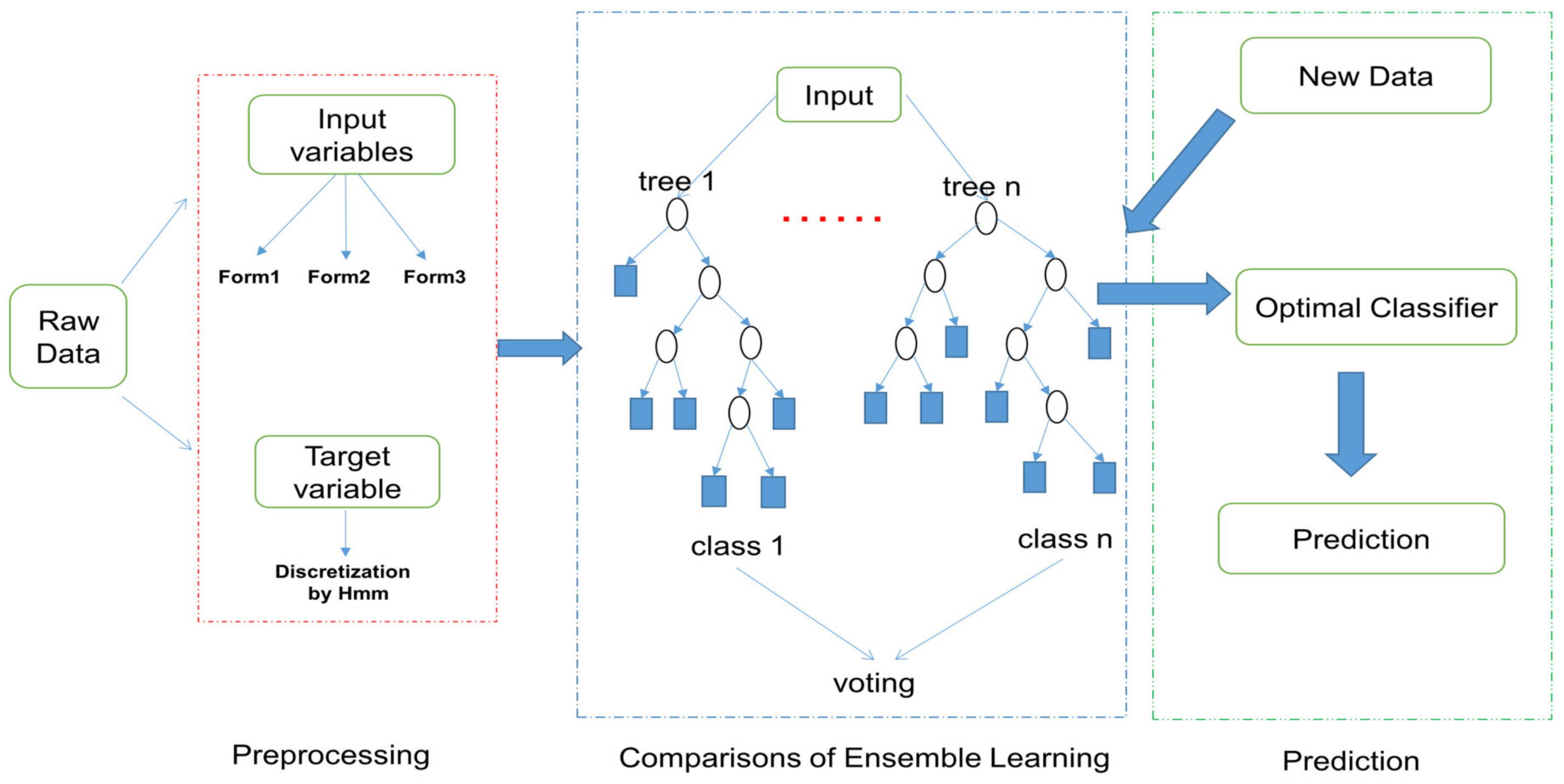
During the tunnel excavation process, predicting the value intervals provides more reliable safety and convenience for the driver and also lays the foundation for the subsequent development of a unified model for different geological conditions. With the aim of predicting the value intervals of cutterhead torque and total thrust, a hybrid prediction model combining HMM and ensemble learning is proposed. The architecture of the hybrid prediction model is shown in Figure 1, and it mainly consists of three stages: data preprocessing, model comparisons, and prediction of target variables. To begin with, we preprocess the data to extract normal excavation data and select the input variables. Then, we discrete those parameters into different states by means of HMM encoding and record their corresponding value intervals. After that, we select the optimal model by comparing the performances of ensemble learning methods under different input forms. Finally, based on the optimal model, we predict the states of the target variables for the new data and extend to validation under different geologies. The detailed descriptions of each stage are presented as follows.

3.1. Data Preprocessing

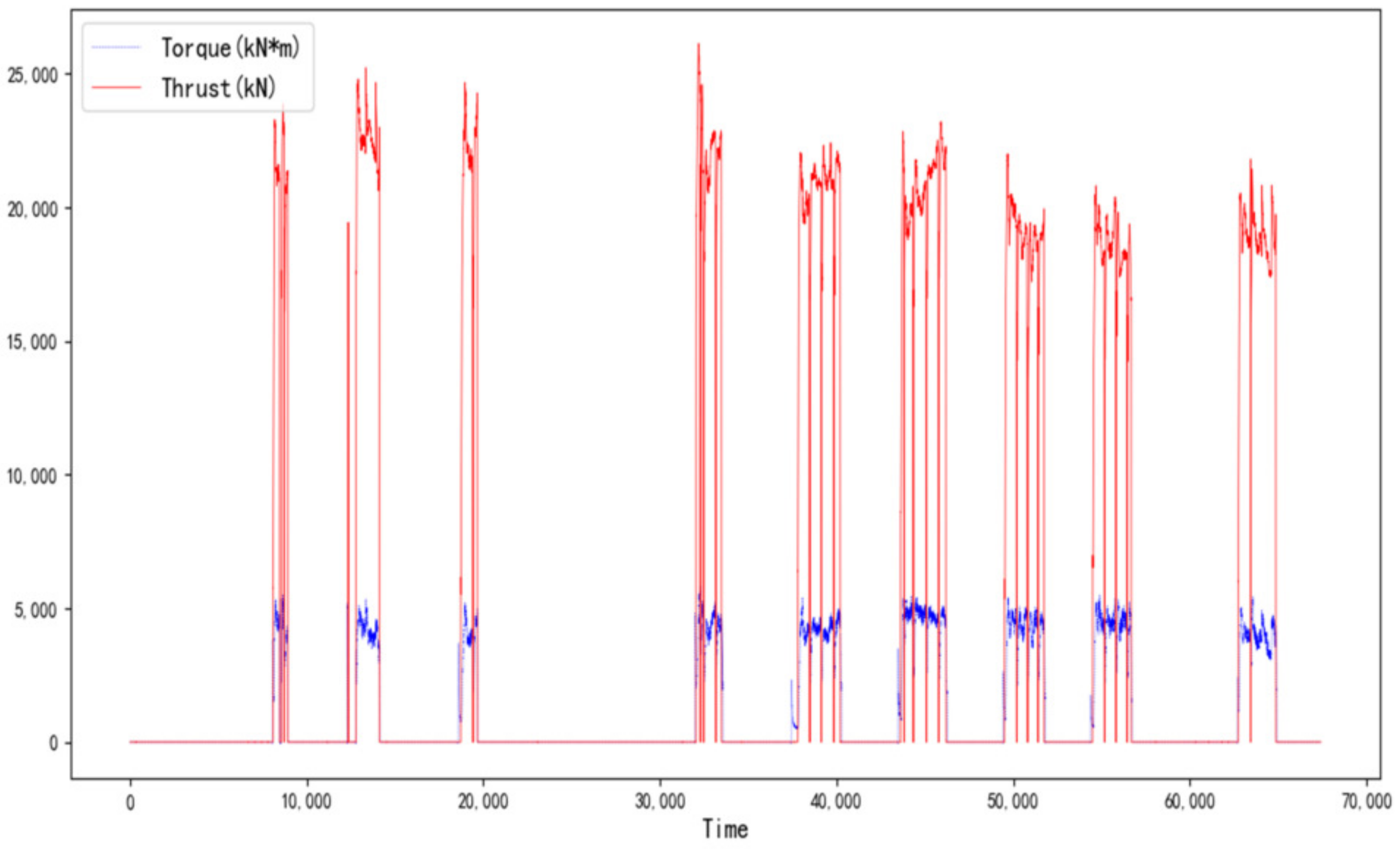
It is noteworthy that TBMs have complex systems including the trust hydraulic cylinder, propel system, other articulated systems, etc., but the boring process has a similar statistical pattern that consists of a series of tunneling cycles. The data in Beijing are plotted as an illustration in Figure 2 to intuitively understand the TBM tunneling process.

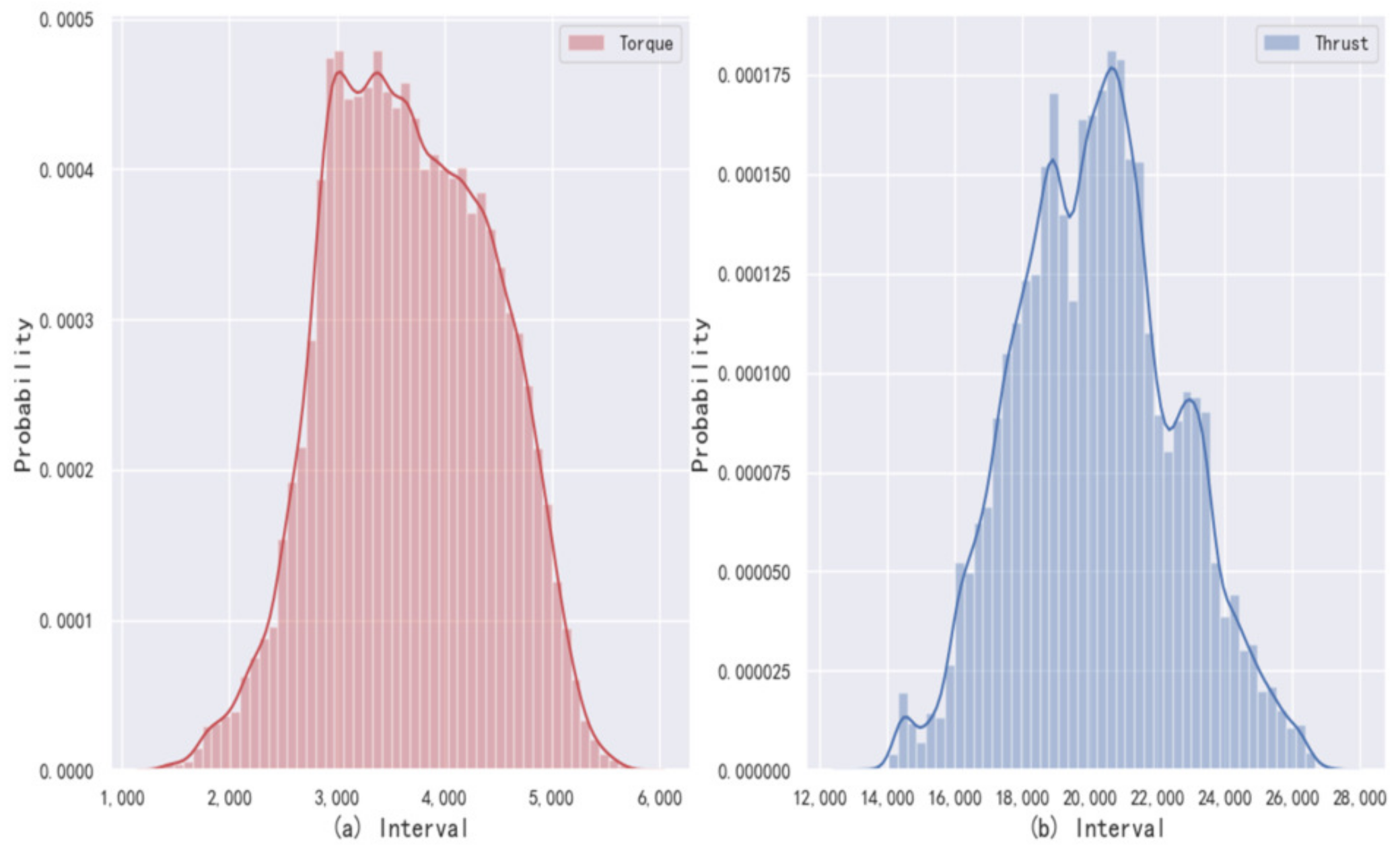
As we can see in Figure 2, TBM sequentially goes through the stages of starting, excavation, pause, ⋯, excavation, and stop during the construction process. In the pause or stop stage, the values of the operating parameters are 0 and they are invalid values in the raw data. In order to predict the cutter torque and thrust more accurately, it is necessary to extract the data of excavation stage from the raw data [12,16,17]. It is noted that the data of the normal excavation stage are relatively smooth within a certain value range, which is significantly different from the starting and shutdown stages, where the starting stage has a clear upward trend and the shutdown stage has a downward trend. In this paper, the linear regression model of the change point detection method is used to find out the change point from one stage to the next based on the different features of the shield parameters in each stage [12]. Undeniably, in the above process, anomalous data can interfere with the determination of change points, but this interference is insignificant because change point detection is based on motion trends and a large number of data samples. Therefore, a limited amount of anomalous data do not have a significant impact. The statistical histograms of cutter torque and thrust in the excavation stage are shown in Figure 3.

Most of the data in the pause stage and start-up stage are removed by using the change point detection. Figure 3 shows that the data in the excavation stage are approximately subject to the normal distribution. The $3\sigma$ principle is applied to remove the outlines to further improve the data quality.

With the objective of predicting the cutterhead torque and total thrust in this paper, the selection of input parameters is particularly important and directly affects the prediction effect. Generally speaking, the data patterns cannot be portrayed by a few variables, but in the case of redundant variables, it may cause over-fitting and affect the generalization ability of the model. Especially, the data in the excavation stage derived from the actual tunnel construction have about 500 attributes. Hence, it is particularly significant to select a few important variables as the input vector from those attributes. Fortunately, the prediction problem is simplified to a classification, and a large number of physical parameters are less relevant to the target parameters, which provides the possibility to efficiently select the input variables to control the dimension of the input vector. This paper aims to construct the prediction model of cutterhead torque and thrust with as few and essential parameters as possible. By comprehensive research on excavation sites and literature references, 7 variables including rotation speed of cutter, advance velocity, rotation speed of screw conveyor, and propelling pressure of four groups are selected as the input variables for the hybrid prediction model. They are all critical and essential for the tunneling stage of the TBMs regardless of the geological conditions. On the one hand, by observing the operation of the driver at the subway tunnel excavation site, these 7 parameters are the most direct and critical in the panel to adjust the tunneling process for the driver. On the other hand, according to the references mentioned in this paper, the input variables are selected in two ways: one is a manual subjective selection (such as Refs. [8,9,10,11,12,13,14]), and the other uses dimensionality reduction methods such as principal component analysis (Ref. [18]). Either way, these 7 parameters are the most frequently used in predicting the torque and thrust, which indicates their importance. Notice that cosine similarity was often used in the above papers to filter out variables that are closely related to the target variables. It should be noted that cosine similarity portrays a linear relationship between attributes of the TBM, but the TBM systems are complex, and it is not sufficient to consider only the linear correlation of attributes. The cosine similarities between those seven TBM attributes and torque are 0.72, 0.56, 0.61, 0.86, 0.87, 0.81, and 0.70, while their cosine similarity with thrust is 0.50, 0.77, 0.75, 0.96, 0.96, 0.96, and 0.85, respectively. Hence, ensemble learning models combined with HMM encoding are employed to mine the nonlinear relationships between those critical attributes of the TBM. On this basis, with the target parameters, cutterhead torque and total thrust as the output variables, a new data set with $T\times 9$ is obtained, and the former seven are input variables. Moreover, three typical models based on the ensemble learning approach are compared.

3.2. Forms of the Model Comparisons

To compare the three kinds of representative ensemble learning models, the different forms of the input variables are designed below. Specifically, for the given dataset $X=\{\overrightarrow{x_1},\cdots ,\overrightarrow{x_i},\cdots ,\overrightarrow{x_d},\overrightarrow{y}\},\overrightarrow{x_i}={(x_{i1},\cdots ,x_{iT})}^T,\overrightarrow{y}={(y_1,\cdots ,y_T)}^T$, where $1\le i\le d$, $d=7$ is the number of input variables, and T is the length of each variable sequence. With this expression, the original input vector is $\overrightarrow{x_t}=(x_{t1},\cdots ,x_{td}),1\le t\le T$, which indicates the values of input vector at time t, and $y_t$ is the corresponding output value. It is noteworthy that an HMM model is employed to extract the hidden states of the variables, and thus, the variables have been discretized. On this basis, all three different forms of the input variables are given as follows for this hybrid prediction model.

(1) The input vector is original $\overrightarrow{x_t}=(x_{t1},\cdots ,x_{td}),1\le t\le T$, and the output $y_t^{{}^{\prime }}$ is the hidden state of target variable that is obtained by HMM;

(2) The input vector is discretized by HMM ${\overrightarrow{x_t}}^{{}^{\prime }}=(x_{t1}^{{}^{\prime }},\cdots ,x_{td}^{{}^{\prime }}),1\le t\le T$, and the output $y_t^{{}^{\prime }}$ is also discretized by HMM;

(3) The input vector is discretized and transformed into OneHot form ${\overrightarrow{x_t}}^{{}^{″}}=(x_{t1}^{{}^{″}},\cdots ,x_{td}^{{}^{″}}),1\le t\le T$, while the output $y_t^{{}^{\prime }}$ is the same as above.

OneHot is a data preprocessing technique that converts categorical variables into binary vectors, which can extend the feature dimension and improve the learner to some extent. As a conclusion, the above different forms of the same seven attributes are used to validate the prediction models based on HMM and ensemble learning. The detailed descriptions of HMM and ensemble learning are presented as follows.

3.3. Hidden Markov Model

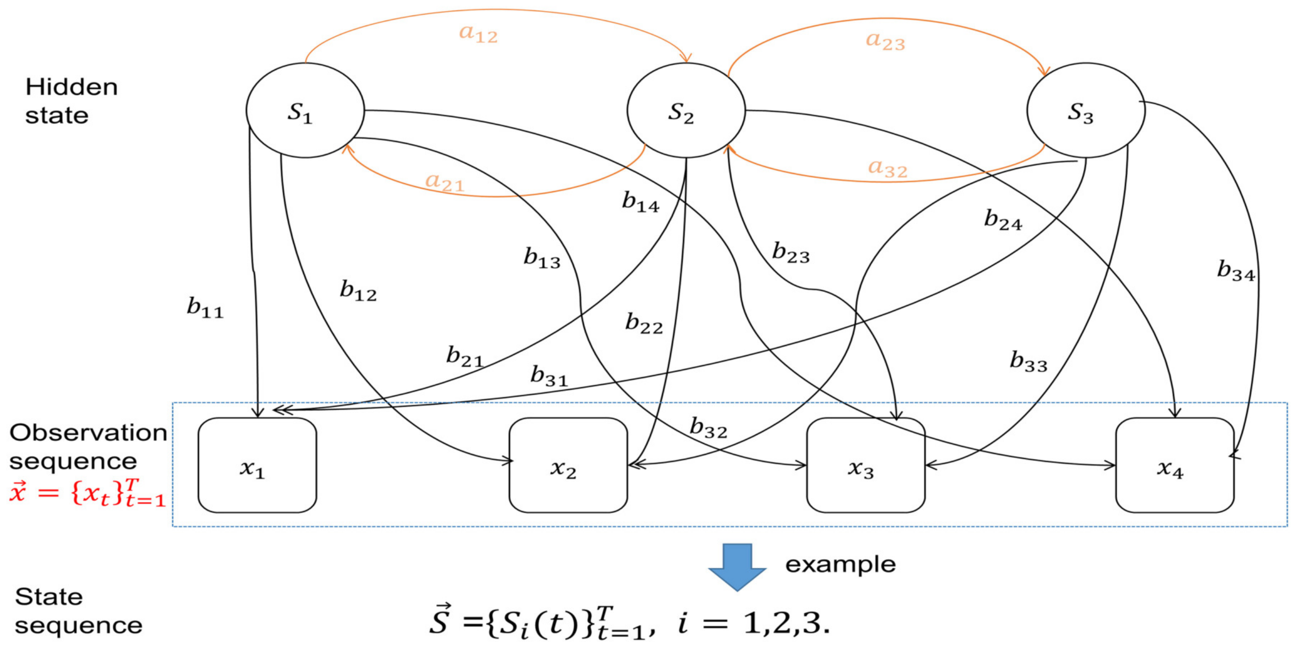
Hidden Markov Model (HMM) is a classical machine learning model that describes a Markov process with implicitly unknown parameters [19]. Recently, HMMs have been used to analyze problems with uncertainty in transportation engineering and the prediction of tunnel geology [20,21,22], because it can capture the probability characteristics of the transitions between the underlying states. The HMM method in this paper is designed to encode variables into discrete states. The schematic of HMM is in Figure 4 and the details are described as follows. For any HMM model, it is composed of three elements: the initial state probability distribution ${\pi }_i=p(i=1)$, state sequence $\overrightarrow{S}={\left\{S_i\left(t\right)\right\}}_{t=1}^T(i=1,\cdots ,N_s)$, and observation sequence $\overrightarrow{x}={\left\{x_t\right\}}_{t=1}^T$, where $N_s$ is the number of hidden state values $S_i$ that can take at the state i and T is the length of the observation sequence. Under the assumption, the complete set of HMM parameters is described by a triplet $\lambda =\{\pi ,A,B\}$, where $\pi ={\left\{{\pi }_i\right\}}_{i=1}^{N_s}$ is the prior initial probability matrix, $A={\left\{a_{ij}\right\}}_{i=1,j=1}^{N_s,N_s}$ is the state transition probability matrix and $B={\left\{b_i\right\}}_{i=1}^{N_s}$ is the observation emission probability matrix where $b_i$ is the emission probability, that is, $b_i\left(x_t\right)=p\left(x_t\right|S_i)$.

Our goal of using HMMs in this paper is to encode variables into discrete states, that is, find the optimal hidden state sequence $\overrightarrow{S}={\left\{S_i\left(t\right)\right\}}_{t=1}^T(i=1,\cdots ,N_s)$ by regarding the operating parameters of TBM as given observation sequences. To achieve this, the Viterbi algorithm was a known method to solve the problem analytically by dynamic programming [23] when the observation sequence $\overrightarrow{x}={\left\{x_t\right\}}_{t=1}^T$ and model $\lambda =\{\pi ,A,B\}$ were given. Therefore, model parameters should be estimated at first by using the Baum–Welch algorithm [24] based on the given observation sequence $\overrightarrow{x}={\left\{x_t\right\}}_{t=1}^T$. For the given operating parameters of TBM, to better analyze their hidden states, an HMM model is designed, and the number of hidden state values $N_s$ is set to different values in Section 4.1.

3.4. Ensemble Learning

Ensemble learning, known as a multiple classifier system, trains and combines multiple learners to solve a learning problem [25]. Nowadays, it is one of the most commonly used machine learning algorithms in engineering applications. Current ensemble learning methods can be roughly grouped into two categories according to the dependencies between multiple learners. One is represented by Boosting and the other is Bagging [26]. AdaBoost is the most well-known Boosting algorithm with strong dependencies between its individual learners, while RF and ERT are Bagging algorithms with decision trees as basis weak learners, and each learner is independent. In order to understand the rules of the model proposed in this paper, the ideas of the AdaBoost, RF, and ERT algorithms are briefly described below.

3.4.1. AdaBoost

AdaBoost was first designed by Freund and Shapire to find a binary classifier [27]. Its theoretical basis is sound and implementation is simple. Nowadays, it has been widely applied to the classification problems. The basic idea of AdaBoost is to learn a small number of weak classifiers h by iteratively and then combining them into a strong one H. Let $H=\left\{h_f\right\}$ be the set of weak classifiers and a given dataset $X=\{(x_1,y_1),\cdots ,(x_T,y_T)\}$, where $x_i\subseteq {\mathrm{R}}^n,y_i\in \{+1,-1\}$, and T is the size of dataset. Let $\{{\omega }_1,\cdots ,{\omega }_T\}$ be the sample weights that reflect the importance degrees of the samples. The technical details of AdaBoost are described as below.

(1) Normalize the weights ${\omega }_i\left(1\right)(i=1,\cdots ,T)$ satisfying ${\sum }_{i=1}^T{\omega }_i\left(1\right)=1.$

(2) For $n=1,\cdots ,N$ execute the following operations:

① The error ${ϵ}_j$ of a weak classifier $h_j$ is the sum of the weighted classification errors,

$${ϵ}_j=\sum _{i=1}^T{\omega }_i\left(n\right)\mathbf{I}[y_i\ne h_j\left(x_i\right)]$$

(1)

where $\mathbf{I}\left[\gamma \right]=\left\{\begin{array}{cc}1\hfill & \gamma =True\hfill \\ 0\hfill & \gamma =False\hfill \end{array}\right.$. Choose the weak classifier $h_n$ with the lowest error ${ϵ}_j$,

$$h_n=arg\underset{h_j\in H}{min}{ϵ}_j.$$

(2)

② Calculate the sum of the weighted classification errors $ϵ\left(n\right)$ for the chosen weak classifier $h_n$.

③ Let

$$\alpha \left(n\right)=\frac{1}{2}log\left(\frac{1-ϵ\left(n\right)}{ϵ\left(n\right)}\right).$$

(3)

④ Update the weights by

$${\omega }_i(n+1)=\frac{{\omega }_i\left(n\right)exp(-\alpha \left(n\right)y_i{h}_n\left(x_i\right))}{Z\left(n\right)},$$

(4)

where $Z\left(n\right)$ is a normalization factor

$$Z\left(n\right)=\sum _{t=1}^T{\omega }_t\left(n\right)exp(-\alpha \left(n\right)y_t{h}_n\left(x_t\right)).$$

(5)

(3) Output the strong classifier

$$H\left(x\right)=sign\left(\sum _{n=1}^N\alpha \left(n\right)h_n\left(x\right)\right)$$

(6)

In each iteration, the weights of the data misclassified are increased but the weights of the data correctly classified are decreased, which in turn changes the weights of the weak classifier. Finally, a linear combination of weak classifiers is combined to form a strong classifier, in which the classifier with a small error rate has a large weight and the classifier with a large classification error rate is given a small weight.

3.4.2. Random Forest (RF)

RF is an extension of Bagging based on bootstrap sampling, where randomized feature selection is introduced on top of Bagging [28]. It is easy to implement and has surprisingly good performance in multi-classification applications. Therefore, it is honored as a representative ensemble learning method and is selected for predicting the key parameters of TBM in this paper. In RF, a decision tree, i.e., CART (classification and regression trees), is used as a weak learner. The implementation of the RF algorithm is summarized as the following 4 steps:

(1) Sample points from datasets in a put-back manner to generate the training set, and the remaining unsampled points are used as the test set;

(2) Randomly select m variables at each node to generate a CART;

(3) Repeat the above steps to form k CARTs;

(4) Integrate the above CARTs and vote the predicted values.

Specifically, traditional decision trees select an optimal split feature from the feature set of each node, whereas RF selects from a subset of m features randomly generated from the feature set of the node [29]. The parameter m controls the randomness and it is given in advance by correlation analysis of the data set. The number of CART k is considered as the key parameter of RF and influences the model performance. In this paper, the parameter k is manually selected to predict the cutter torque and total thrust by the RF model.

3.4.3. Extreme Random Tree (ERT)

The ERT model is proposed by Geurts et al. [30] and has been widely used for prediction problems as being computationally efficient. Similar to the RF, it is powerful for the multi-classification and is able to handle high-dimensional feature vectors. The algorithm has two key points:

(1) ERT uses all training samples to construct each tree with varying parameters rather than the bagging procedure used in RF;

(2) ERT randomly chooses the node split upon the construction of each tree, rather than the best split used in RF.

In general, AdaBoost improves the model accuracy by adjusting the weights of misclassified data points, and the weights of each weak classifier are different. In contrast, RF and ERF learn classifiers by random sampling with put-back, where the weights of each classifier are the same, and the final classification result is determined by voting. In conclusion, they all have a good ability to learn classifiers for classification problems and are easily implemented in Python. Therefore, for the prediction of the discrete state of cutterhead torque and total thrust, the three models mentioned above including AdaBoost, RF, and ERT are established after the cutterhead torque and thrust encoded by HMM. The generalization abilities of those models for the prediction are compared in Section 4.2.

3.5. Performance Evaluation Metric

After the predicted models are established, some statistical metrics including confusion matrix, accuracy, precision, and recall are calculated to evaluate the performance of the prediction models. The definition of the confusion matrix for multiclass classification is shown in the following

Table 1. The confusion matrix of multiclass classification.

		Predicted Class
		Class 1	⋯	Class j	Class n
True	class 1	$k_{11}$	⋯	$k_{1j}$	$k_{1n}$
	⋯	⋯	⋯	⋯	⋯
	class i	$k_{i1}$	⋯	$k_{ij}$	$k_{in}$
	class n	$k_{n1}$	⋯	$k_{nj}$	$k_{nn}$

.

where $k_{ij}(1\le i,j\le n)$ indicates the number of predicted class j when the true class is i, and n is the number of classes. The confusion matrix presents the number of predicted and true classes separately, and it visualizes the performance of predictions on each class. Based on this, the accuracy, precision, and recall of the classifier are calculated separately as shown below. The accuracy is defined as below:

$$A_{cc}=\frac{{\sum }_{i=1}^n{k}_{ii}}{{\sum }_{i=1}^n{\sum }_{j=1}^n{k}_{ij}}.$$

(7)

The precision, recall are defined as follows, respectively:

$$p_i=\frac{k_{ii}}{{\sum }_{i^{{}^{\prime }}=1}^n{k}_{i^{{}^{\prime }}i}},r_i=\frac{k_{ii}}{{\sum }_{j=1}^n{k}_{ij}},$$

(8)

where $p_i$ represents the ratio of the number of samples with correct predictions in class i to the samples whose predicted values are i class, and $r_i$ is the ratio of the number of samples predicted to be correct for class i to the samples that are actually class i. Unfortunately, precision and recall are contradictory. To eliminate this drawback, an alternative performance measure that considers precision and recall simultaneously is defined as:

$$f_i=\frac{2\times p_i\times r_i}{p_i+r_i}.$$

(9)

4. Case Study

4.1. Hmm Analysis

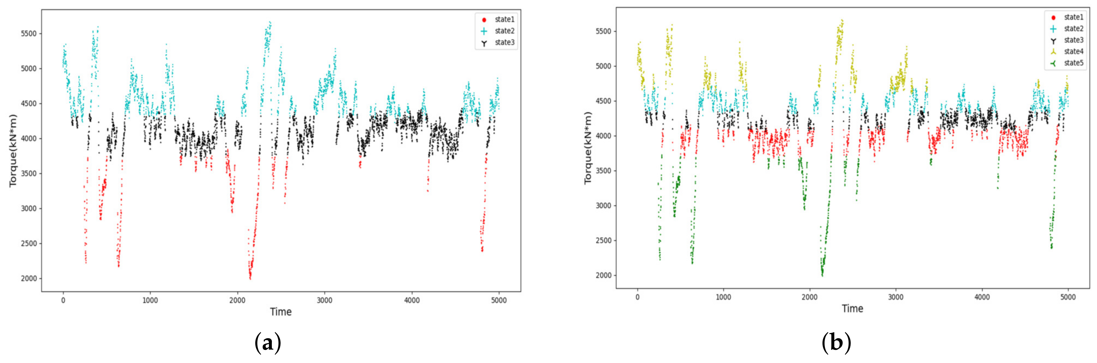
For the given data set of excavation stage, the values of each parameter are continuous and the target variables (torque and thrust) are approximately subject to the Gauss distribution, which has been illustrated in Figure 3. As mentioned in Section 3.1, a total of nine parameters are used as input and output variables for the proposed prediction model. Therefore, a Gaussian distribution $G_i=\{{\mu }_i,{\sigma }_i^2\}(1\le i\le 9)$ is modeled as the probability function to estimate the HMM parameters. Take the excavation data in Beijing as an example, from the perspective of the practical application in assisted shield tunnels, the number of hidden states is set as $N_s=$ 3 and 5 to analyze the discretization results of the target variables by HMM encoding, respectively. For the torque, the performance of the GaussHMM encoding with $N_s=3$ is shown in Figure 5a, and the case of $N_s=5$ is plotted in Figure 5b.

A total of 5000 data are used to analyze the effects of HMM. As shown in Figure 5a, the cutterhead torque is encoded into three hierarchical states and has a strong statistical pattern. This is similar to the case of five states, as shown in Figure 5b. The middle state is relatively stable, which can be regarded as safe, but the other states fluctuate widely that need to be alerted for the operator.

Table 2. Analysis of torque by HMM.

${\mathit{N}}_{\mathit{s}}$	Mean	Variance	Value Interval 1	Number
3	(3122, 4074, 4640)	(262,187, 26,269, 80,482)	(${\mathbf{1}}_{1993}^{3738}$, ${\mathbf{2}}_{3630}^{4330}$, ${\mathbf{3}}_{4225}^{5661}$)	(636, 2332, 2032)
5	(3078, 3943, 4223, 4482, 4939)	(250,285, 11,203, 6378, 9349, 62,091)	(${\mathbf{1}}_{1993}^{3785}$, ${\mathbf{2}}_{3662}^{4160}$, ${\mathbf{3}}_{4037}^{4416},$, ${\mathbf{4}}_{4289}^{4751}$, ${\mathbf{5}}_{4630}^{5661}$)	(592, 1289, 1163, 1228, 728)

¹${\mathbf{k}}_a^b$, where a is the minimum value and b is the maximum value of the hidden state k.

presents the mean, variance, interval, and the number of samples for each state. It is found that when states are sorted by their mean in numerical order, the middle state has the smallest variance and contains the most number of samples.

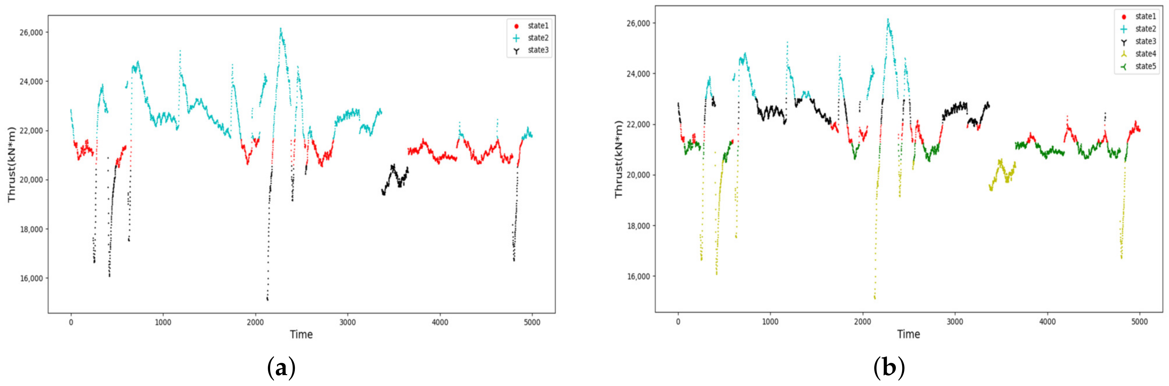
For the thrust, the hidden states under $N_s=3$ and 5 are depicted in Figure 6. Specifically, the detailed statistics of each state are presented in

Table 3. Analysis of thrust by HMM.

${\mathit{N}}_{\mathit{s}}$	Mean	Variance	Value Interval	Number
3	(19,306, 21,303, 22,867)	(1,591,975, 72,051, 832,036)	$({\mathbf{1}}_{15126}^{20887}$, ${\mathbf{2}}_{20516}^{21666}$, ${\mathbf{3}}_{21624}^{26141}$)	(574, 1920, 2506)
5	(19,312, 20,967, 21,602, 22,513, 23,947)	(1,592,170, 31,831, 51,552, 71,654, 532,402)	(${\mathbf{1}}_{15126}^{20887}$, ${\mathbf{2}}_{20516}^{21373}$, ${\mathbf{3}}_{4037}^{4416},$ ${\mathbf{4}}_{21238}^{22328}$, ${\mathbf{5}}_{22929}^{26141}$)	(595, 1365, 971, 1272, 817)

. Similar to the torque, the thrust can be discretized into hierarchical states by HMM, as shown in Figure 6. For the hidden state 5, its three intermediate states can all be considered safe, and it gives the driver a finer range of values compared to hidden states 3. In practice, the number of hidden states can be subjectively set to three or five depending on the driver’s specific operating habits. The discretization process does not change the frequency of the data, and the frequency of the discretized data remains the same as the normal data collection frequency of the excavation stage, which is 5 s, as mentioned in Section 2. This ensures that the number of data samples before and after discretization is consistent, allowing the model to hold when the input variables are in raw form and the output variables are discretized. Meanwhile, we have noticed that the intervals corresponding to the adjacent hidden states have a little overlap. However, there is no serious interference because the overlap is very limited. If necessary, the overlap can be eliminated by calculating the average of the overlapping parts as the interval boundary.

4.2. Performances of the Ensemble Learning Models

Under the pebble geological conditions in Beijing, a total of 8487 samples in the excavation stage are used as an illustration, and $70\%$ of them constitute the training set and the rest are used as the test set. The $A_{cc}$ values of the prediction models for the cutterhead torque in different forms of input variables are presented in

Table 4. The $A_{cc}$ of models for the torque prediction in different forms of input variables.

Forms		AdaBoost		RF		ERT
		Train	Test	Train	Test	Train	Test
Raw	3	1.00	0.85	1.00	0.91	1.00	0.92
	5	1.00	0.75	0.99	0.83	1.00	0.85
HMM	3	0.74	0.71	0.79	0.76	0.79	0.76
OneHot	3	0.66	0.60	0.78	0.76	0.78	0.76

. From Table 4, it is seen that the three representative models of ensemble learning all have high accuracy for the classification prediction of cutterhead torque. For the three different input forms, the prediction accuracies of the three models are all above $0.70$ except for the case of AdaBoost in OneHot form. Among them, the accuracy of the ERT model is the highest, $0.92$, when the input variables are in the Raw form and the torque is discretized into three states. By comparing the three different input forms, the accuracy is the highest in the Raw form, and the torque prediction is slightly better when it is in three classes compared to five classes. For the three representative ensemble learning models, the prediction of ERT is almost the same as the RF model and significantly better than AdaBoost.

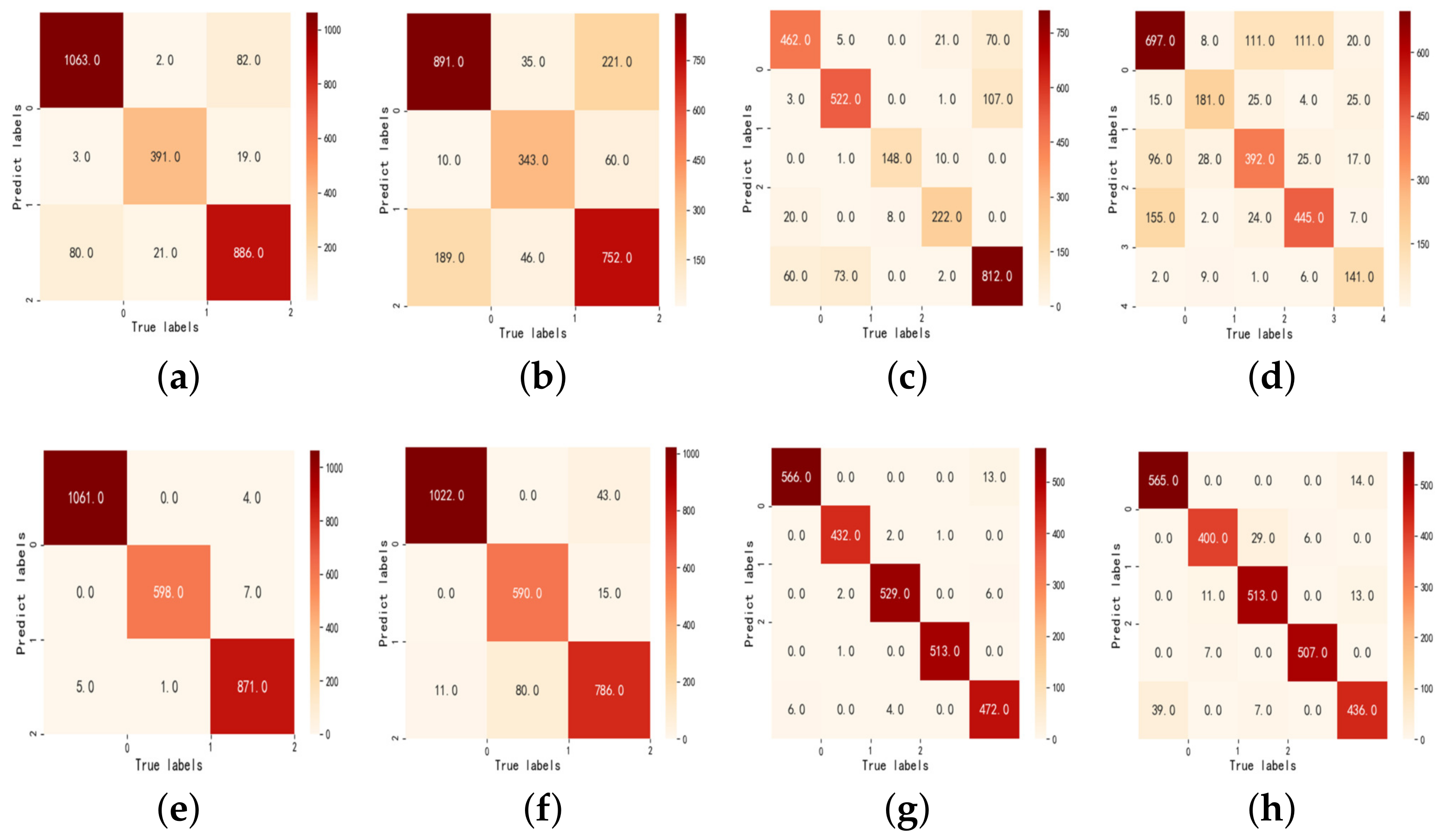
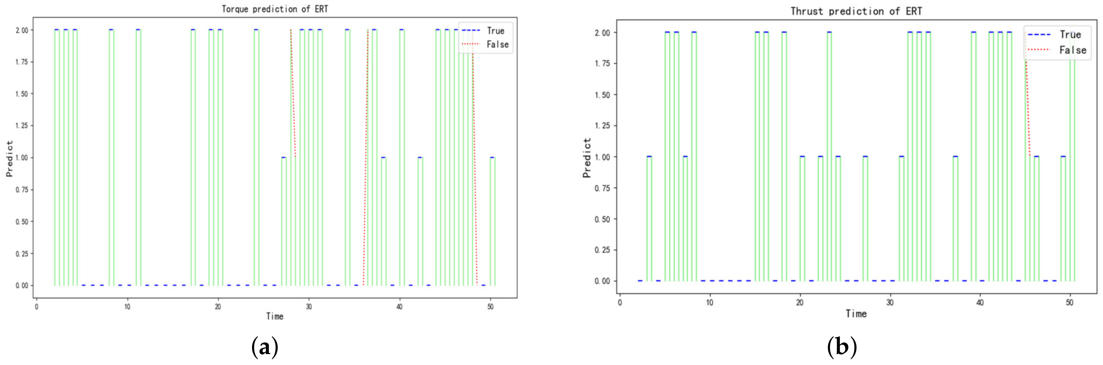
The confusion matrices for different cases of the ERT model are shown in Figure 7. It can be intuitively seen that the performance of the ERT model is optimal when the input variables are in Raw form and torque is into three classes. The prediction of the torque in three classes is better than five classes regardless of whether the input variables are encoded by HMM.

Table 5. The statistical performance of ERT for the torque prediction.

Class		AdaBoost			RF			ERT			N(2547)
		${\mathit{p}}_{\mathit{i}}$	${\mathit{r}}_{\mathit{i}}$	${\mathit{f}}_{\mathit{i}}$	${\mathit{p}}_{\mathit{i}}$	${\mathit{r}}_{\mathit{i}}$	${\mathit{f}}_{\mathit{i}}$	${\mathit{p}}_{\mathit{i}}$	${\mathit{r}}_{\mathit{i}}$	${\mathit{f}}_{\mathit{i}}$
3	1	0.88	0.87	0.87	0.92	0.91	0.92	0.92	0.93	0.93	1147
	2	0.83	0.81	0.82	0.88	0.89	0.88	0.90	0.89	0.90	987
	3	0.85	0.91	0.88	0.94	0.93	0.93	0.95	0.95	0.95	413
	ave	0.85	0.85	0.85	0.91	0.91	0.91	0.92	0.92	0.92
5	1	0.74	0.82	0.78	0.85	0.85	0.85	0.87	0.88	0.87	250
	2	0.73	0.75	0.74	0.79	0.85	0.82	0.82	0.86	0.84	947
	3	0.74	0.71	0.72	0.83	0.79	0.81	0.85	0.82	0.84	558
	4	0.77	0.75	0.76	0.86	0.80	0.83	0.87	0.82	0.84	633
	5	0.87	0.79	0.83	0.91	0.90	0.90	0.93	0.93	0.93	159
	ave	0.75	0.75	0.75	0.83	0.83	0.83	0.85	0.85	0.85

lists the statistical metrics of each state on the testing data for intuitive comparisons, where the input variables are in Raw form and the torque hidden states are set as $N_s=3$ or 5. From Table 5, there is no significant difference between the identification statistical performance of each class, which suggests that it is feasible to predict the target variables that are encoded as discrete states. The metrics on all states are above $0.71$ with most of them being greater than $0.85$. The results indicate that the discrete states of the torque after encoding can be well predicted by using ensemble learning models in the Raw form of input. To visualize the prediction results, the actual and predicted torque using the ERT model in the Raw form input under the hidden state $N_s=3$ is plotted in Figure 8a. In brief, the ERT model outperforms RF and AdaBoost for the torque prediction, and the input of Raw form is optimal.

Next, for the other target variable thrust, comparisons of the performances of the proposed hybrid model are shown in the following. The $A_{cc}$ and the statistical metrics of each state for the thrust prediction models based on ensemble learning are listed in

Table 6. The $A_{cc}$ of models for the thrust prediction in different forms of input variables.

Forms		AdaBoost		RF		ERT
		Train	Test	Train	Test	Train	Test
Raw	3	0.99	0.98	1.00	0.99	1.0	0.99
	5	0.99	0.98	1.00	0.99	1.00	0.99
HMM	3	0.92	0.90	0.95	0.94	0.96	0.95
OneHot	3	0.72	0.71	0.95	0.94	0.95	0.94

and

Table 7. The statistical metrics of each state for the thrust prediction models.

Class		AdaBoost			RF			ERT			N(2547)
		${\mathit{p}}_{\mathit{i}}$	${\mathit{r}}_{\mathit{i}}$	${\mathit{f}}_{\mathit{i}}$	${\mathit{p}}_{\mathit{i}}$	${\mathit{r}}_{\mathit{i}}$	${\mathit{f}}_{\mathit{i}}$	${\mathit{p}}_{\mathit{i}}$	${\mathit{r}}_{\mathit{i}}$	${\mathit{f}}_{\mathit{i}}$
3	1	0.98	0.99	0.98	1.00	1.00	1.00	1.00	1.00	1.00	1065
	2	0.98	0.98	0.98	0.98	1.00	0.99	0.99	0.99	0.99	877
	3	0.98	0.99	0.98	1.00	0.98	0.99	1.00	0.99	0.99	605
	ave	0.98	0.99	0.98	0.99	0.99	0.99	0.99	0.99	0.99
5	1	0.97	0.97	0.97	0.99	0.99	0.99	0.99	0.99	0.99	435
	2	0.98	0.98	0.98	0.99	0.98	0.99	0.99	0.98	0.99	579
	3	0.97	0.98	0.97	0.98	0.99	0.99	0.99	0.99	0.99	537
	4	0.99	0.99	0.99	0.99	1.00	1.00	1.00	1.00	1.00	514
	5	0.96	0.96	0.96	0.97	0.97	0.97	0.97	0.98	0.97	482
	ave	0.98	0.98	0.98	0.99	0.99	0.99	0.99	0.99	0.99

, respectively. The confusion matrices under different cases and the comparisons between actual and predicted thrust under $N_s=3$ of the ERT model are shown in Figure 7e–h and Figure 8b.

According to Table 6 and Table 7, the $A_{cc}$ values of models are all greater than 0.9 except for the case of AdaBoost in OneHot form and the highest is close to 1, which indicates that the thrust states are predicted very well. From Figure 7e–h, the prediction model with the input variables in Raw form performs more efficiently than the form of HMM, and the thrust prediction in the hidden states $N_s=3$ is slightly better compared to $N_s=5$.

4.3. Another Case

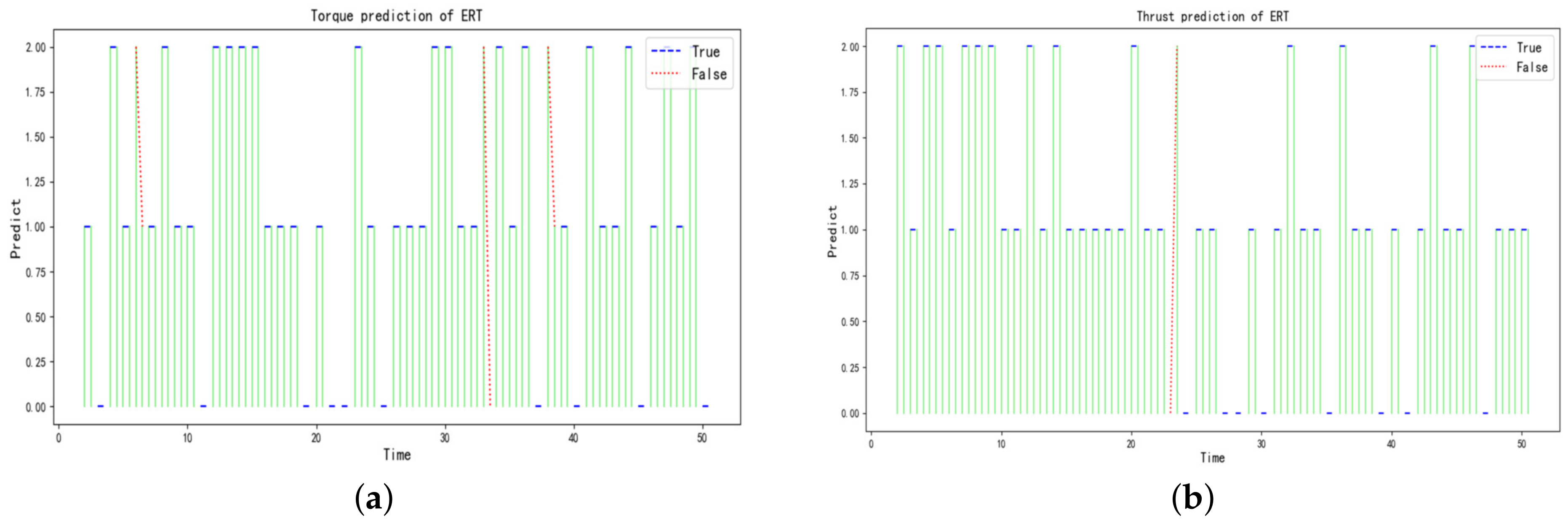
To give a further illustration, the data of Zhengzhou in a fine sand stratum are given as another case to demonstrate the model performance. A total of 27,051 samples in the excavation stage are used, and the ratio of training data to test data is set as $7:3$ by the same as Beijing.

Table 8. The $A_{cc}$ of models for the torque prediction in different forms of input variables.

Forms		AdaBoost		RF		ERT
		Train	Test	Train	Test	Train	Test
Raw	3	1.00	0.89	0.96	0.91	1.00	0.93
	5	1.00	0.79	0.93	0.82	1.00	0.87
HMM	3	0.70	0.70	0.71	0.71	0.71	0.71
OneHot	3	0.56	0.55	0.71	0.71	0.71	0.71

and

Table 9. The $A_{cc}$ of models for the thrust prediction in different forms.

Forms		AdaBoost		RF		ERT
		Train	Test	Train	Test	Train	Test
Raw	3	1.00	0.99	1.00	0.99	1.0	0.99
	5	1.00	0.98	1.00	0.99	1.00	0.99
HMM	3	0.95	0.94	0.95	0.95	0.95	0.95
OneHot	3	0.81	0.80	0.95	0.95	0.95	0.95

present the $A_{cc}$ of prediction models with input variables in different forms for the cutterhead torque and thrust, respectively. The comparisons between the actual and predicted states of target variables under $N_s=3$ of the ERT model are presented in Figure 9.

Table 4 and Table 8 show that the classifier reached an accuracy of 1 on the training dataset and it does not perform as well on the test dataset when using raw input for the torque. The reason may be that the input data in their raw form contain sufficient information to make the target classes fully separable on the training set. However, because there is a little overlap in the target intervals when discretizing, which causes misclassification of the target classes, the target classes are not fully separable on the test set. In addition, when the input form is HMM, the accuracies on the training and test sets are close, which is because the discretization loses some information to some extent to avoid over-fitting on the training set. Specifically, when the input variables are HMM, some information is lost so that the target categories are not completely separated on the training set as in the raw input form, so the accuracy is lower than the raw form, but the over-fitting is avoided so that the accuracy is close on the training and test sets. It is also noted that the prediction accuracy of the classifier is close on the training and test sets for the thrust, but for the cutterhead torque, there is better performance on the training set than on the test set. This may be since more intervals overlap when the cutterhead torque is discretized than the thrust, as well as the fact that the thrust is more easily inscribed by the selected input variables.

5. Discussion

In this study, the data in the excavation stage are extracted firstly, and then, the thrust and torque of the excavation stage are discretized into hierarchical states by HMM. Figure 5 and Figure 6 illustrate that the hidden states of the torque and thrust have a statistical pattern, i.e., the current state derives from the previous moment. This is consistent with the fact that the parameters are heavily influenced by their own inertia during the excavation stage. Therefore, the discretization of the torque and thrust by the HMM model is reasonable for discovering the hidden states of the variable themselves, and it is attributed to reducing the complexity of predicting the variables compared to deep learning algorithms. Meanwhile, it is worth noting that the outliers and noises, e.g., abrupt jump points, may negatively affect the discretization, and efforts are needed to identify those outliers and noises in further research.

For the excavation data in Zhengzhou, Table 8 and Table 9 show that the hybrid proposed models have a higher accuracy for the torque and thrust prediction compared with Beijing. The main reason may be that there are more training data and fewer noises in Zhengzhou, and the relationship between variables is relatively easy to learn. Although there is some difference in the accuracy of the predictions, there are some statistical laws that exist. When the input variables are in the Raw form, the prediction model performs more efficiently than the HMM form, and the prediction in the HMM form is approximated to the OneHot form. The main reason lies in that the input variables would lose some feature information in the process of discretization by HMM, and the OneHot form can not increase the effective information, although it formally extends the dimensionality of the input variables compared with the form of HMM.

In general, it is effective to encode the target variables into discrete states by HMM and transform the prediction into a classification problem. The results validate the prediction performance and the generalization ability of the proposed method under different geological conditions. The discretized intervals of cutter torque and thrust, although some information may be lost, still reflect the degree of obstruction and excavation behavior of geological conditions. It is worth noting that compared with the previous data-driven models, the proposed model with good performance has only seven parameters as input variables, and those seven parameters are panel set parameters that can be adjusted by the operator. Therefore, we aim to further match the corresponding geological conditions by establishing the coupling relationship between the value intervals of cutterhead torque, thrust and panel set parameters, which provides the basis for adjusting the panel operating parameters to geological conditions. It is of great meaning in the practical application of intelligent TBM tunneling, and efforts will be needed.

6. Conclusions

In this paper, to accomplish the mapping between essential parameters of TBMs and assist intelligent tunneling, a hybrid prediction model based on HMM and ensemble learning is applied to predicting intervals of the cutterhead torque and total thrust. For the data of the excavation stage, torque and thrust are discretized into different states by employing HMM, and the predictions become classification problems, which provides the basis for reducing the size of the model input to use the essential parameters only. Then, three representative ensemble learning models including AdaBoost, RF, and ERT are used to predict the classification problem, and comparisons have been conducted in three different forms of the same input variables. Two excavation datasets collected from different geological conditions are also used to validate the effectiveness and generalization of the proposed methods. By comparing the performances of the three representative models, ERT with the input parameters in Raw form has the highest accuracy and is selected to predict the torque and thrust. Meanwhile, the results show that (1) the torque and thrust can be efficiently divided into different intervals by HMM; (2) the ERT model outperforms RF and AdaBoost for the prediction of torque and thrust; (3) the input of Raw form is optimal for the prediction models based on the ensemble learning. Therefore, the ERT prediction method combined with HMM can accurately and effectively predict the cutterhead torque and thrust intervals in the practical tunnel boring application, which lays the foundation for subsequent adjustment of panel parameters according to geological conditions.

In the future, efforts will be made to identify outliers and noises in the excavation data and consider the geological conditions.

References

- Yang, B.; Chen, S.; Sun, S.; Deng, L.; Li, Z.; Li, W.; Li, H. Vibration suppression of tunnel boring machines using non-resonance approach. Mech. Syst. Signal Process. 2020, 145, 106969. [Google Scholar] [CrossRef]
- Maidl, B.; Herrenknecht, M.; Maidl, U.; Wehrmeyer, G. Mechanised Shield Tunnelling; John Wiley & Sons: Hoboken, NJ, USA, 2013. [Google Scholar]
- Krause, H. Geologische Erfahrungen beim Einsatz von Tunnelvortriebsmaschinen in Baden-Württemberg. In Neue Erkenntnisse im Hohlraumbau Fundierungen im Fels Latest Findings in the Construction of Underground Excavations Rock Foundations; Springer: Berlin/Heidelberg, Germany, 1976; pp. 49–60. [Google Scholar]
- Ates, U.; Bilgin, N.; Copur, H. Estimating torque, thrust and other design parameters of different type TBMs with some criticism to TBMs used in Turkish tunneling projects. Tunn. Undergr. Space Technol. 2014, 40, 46–63. [Google Scholar] [CrossRef]
- Zhang, Q.; Hou, Z.; Huang, G.; Cai, Z.; Kang, Y. Mechanical characterization of the load distribution on the cutterhead–ground interface of shield tunneling machines. Tunn. Undergr. Space Technol. 2015, 47, 106–113. [Google Scholar] [CrossRef]
- Zhou, X.P.; Zhai, S.F. Estimation of the cutterhead torque for earth pressure balance TBM under mixed-face conditions. Tunn. Undergr. Space Technol. 2018, 74, 217–229. [Google Scholar] [CrossRef]
- Faramarzi, L.; Kheradmandian, A.; Azhari, A. Evaluation and optimization of the effective parameters on the shield TBM performance: Torque and thrust-Using discrete element method (DEM). In Geotechnical and Geological Engineering; Springer: Berlin/Heidelberg, Germany, 2020; pp. 1–15. [Google Scholar]
- Sun, W.; Shi, M.; Zhang, C.; Zhao, J.; Song, X. Dynamic load prediction of tunnel boring machine (TBM) based on heterogeneous in-situ data. Autom. Constr. 2018, 92, 23–34. [Google Scholar] [CrossRef]
- Gao, X.; Shi, M.; Song, X.; Zhang, C.; Zhang, H. Recurrent neural networks for real-time prediction of TBM operating parameters. Autom. Constr. 2019, 98, 225–235. [Google Scholar] [CrossRef]
- Song, X.; Shi, M.; Wu, J.; Sun, W. A new fuzzy c-means clustering-based time series segmentation approach and its application on tunnel boring machine analysis. Mech. Syst. Signal Process. 2019, 133, 106279. [Google Scholar] [CrossRef]
- Leng, S.; Lin, J.R.; Hu, Z.Z.; Shen, X. A hybrid data mining method for tunnel engineering based on real-time monitoring data from tunnel boring machines. IEEE Access 2020, 8, 90430–90449. [Google Scholar] [CrossRef]
- Hong, K.; Li, F.; Zhou, Z.; Li, F.; Zhu, X. A Data-Driven Method for Predicting the Cutterhead Torque of EPB Shield Machine. Discret. Dyn. Nat. Soc. 2021, 21, 11. [Google Scholar] [CrossRef]
- Qin, C.; Shi, G.; Tao, J.; Yu, H.; Jin, Y.; Lei, J.; Liu, C. Precise cutterhead torque prediction for shield tunneling machines using a novel hybrid deep neural network. Mech. Syst. Signal Process. 2021, 151, 107386. [Google Scholar] [CrossRef]
- Jin, Y.; Qin, C.; Tao, J.; Liu, C. An accurate and adaptative cutterhead torque prediction method for shield tunneling machines via adaptative residual long-short term memory network. Mech. Syst. Signal Process. 2022, 165, 108312. [Google Scholar] [CrossRef]
- Xu, C.; Liu, X.; Wang, E.; Wang, S. Prediction of tunnel boring machine operating parameters using various machine learning algorithms. Tunn. Undergr. Space Technol. 2021, 109, 103699. [Google Scholar] [CrossRef]
- Zhang, Q.; Liu, Z.; Tan, J. Prediction of geological conditions for a tunnel boring machine using big operational data. Autom. Constr. 2019, 100, 73–83. [Google Scholar] [CrossRef]
- Chen, H.; Xiao, C.; Yao, Z.; Jiang, H.; Zhang, T.; Guan, Y. Prediction of TBM Tunneling Parameters through an LSTM Neural Network. In Proceedings of the 2019 IEEE International Conference on Robotics and Biomimetics (ROBIO), Dali, China, 6–8 December 2019; pp. 702–707. [Google Scholar]
- Salimi, A.; Rostami, J.; Moormann, C.; Delisio, A. Application of non-linear regression analysis and artificial intelligence algorithms for performance prediction of hard rock TBMs. Tunn. Undergr. Space Technol. 2016, 58, 236–246. [Google Scholar] [CrossRef]
- Chen, P.; Yi, D.; Zhao, C. Trading Strategy for Market Situation Estimation Based on Hidden Markov Model. Mathematics 2020, 8, 1126. [Google Scholar] [CrossRef]
- Leu, S.S.; Adi, T.J.W. Probabilistic prediction of tunnel geology using a Hybrid Neural-HMM. Eng. Appl. Artif. Intell. 2011, 24, 658–665. [Google Scholar] [CrossRef]
- Guan, Z.; Deng, T.; Du, S.; Li, B.; Jiang, Y. Markovian geology prediction approach and its application in mountain tunnels. Tunn. Undergr. Space Technol. 2012, 31, 61–67. [Google Scholar] [CrossRef] [Green Version]
- Yang, Y.; Jiang, J. Adaptive bi-weighting toward automatic initialization and model selection for HMM-based hybrid meta-clustering ensembles. IEEE Trans. Cybern. 2018, 49, 1657–1668. [Google Scholar] [CrossRef]
- Zen, H.; Tokuda, K.; Kitamura, T. A Viterbi algorithm for a trajectory model derived from HMM with explicit relationship between static and dynamic features. In Proceedings of the 2004 IEEE International Conference on Acoustics, Speech, and Signal Processing, Montreal, QC, Canada, 17–21 May 2004; Volume 1, p. I-837. [Google Scholar]
- Dempster, A.P.; Laird, N.M.; Rubin, D.B. Maximum likelihood from incomplete data via the EM algorithm. J. R. Stat. Soc. Ser. B Methodol. 1977, 39, 1–22. [Google Scholar]
- Saleem, F.; Ullah, Z.; Fakieh, B.; Kateb, F. Intelligent Decision Support System for Predicting Student’s E-Learning Performance Using Ensemble Machine Learning. Mathematics 2021, 9, 2078. [Google Scholar] [CrossRef]
- Zhou, Z.H. Ensemble learning. In Machine Learning; Springer: Berlin/Heidelberg, Germany, 2021; pp. 181–210. [Google Scholar]
- Freund, Y.; Schapire, R.E. A decision-theoretic generalization of on-line learning and an application to boosting. J. Comput. Syst. Sci. 1997, 55, 119–139. [Google Scholar] [CrossRef] [Green Version]
- Breiman, L. Random forests. Mach. Learn. 2001, 45, 5–32. [Google Scholar] [CrossRef] [Green Version]
- Hsu, B.M. Comparison of supervised classification models on textual data. Mathematics 2020, 8, 851. [Google Scholar] [CrossRef]
- Geurts, P.; Ernst, D.; Wehenkel, L. Extremely randomized trees. Mach. Learn. 2006, 63, 3–42. [Google Scholar] [CrossRef] [Green Version]
Figure 1.
The architecture of the hybrid prediction model.
Figure 2.
Torque and thrust in the raw data from Beijing.
Figure 3.
The statistical histograms of data in the excavation stage.
Figure 4.
Schematic of the HMM.
Figure 5.
The hidden states of torque: (a) under ; (b) under .
Figure 6.
The hidden states of thrust: (a) under ; (b) under .
Figure 7.
The confusion matrices of the ERT model under different cases (first row: torque; second row: thrust): (a,e) Input variables are in Raw form and output is into 3 classes; (b,f) Input variables are in HMM form and output is into 3 classes; (c,g) Input variables are in Raw form and output is into 5 classes; (d,h) Input variables are in HMM form and output is into 5 classes.
Figure 8.
Comparisons between actual and predicted states of the ERT model under : (a) Torque; (b) Thrust.
Figure 9.