Fast Summarization of Long Time Series with Graphics Processor

Abstract

Summarization of a long time series often occurs in analytical applications related to decision-making, modeling, planning, and so on. Informally, summarization aims at discovering a small-sized set of typical patterns (subsequences) to briefly represent the long time series. Apparent approaches to summarization like motifs, shapelets, cluster centroids, and so on, either require training data or do not provide an analyst with information regarding the fraction of the time series that a typical subsequence found corresponds to. Recently introduced, the time series snippet concept overcomes the above-mentioned limitations. A snippet is a subsequence that is similar to many other subsequences of the time series with respect to a specially defined similarity measure based on the Euclidean distance. However, the original Snippet-Finder algorithm has cubic time complexity concerning the lengths of the time series and the snippet. In this article, we propose the PSF (Parallel Snippet-Finder) algorithm that accelerates the original snippet discovery schema with GPU and ensures acceptable performance over very long time series. As opposed to the original algorithm, PSF splits the calculation of the similarity of all the time series subsequences to a snippet into several steps, each of which is performed in parallel. Experimental evaluation over real-world time series shows that PSF outruns both the original algorithm and a straightforward parallelization.

1. Introduction

Time series data are ubiquitous and important in many subject domains, and are actively utilized in a large number of analytical applications related to decision-making, modeling, planning, and so on. Summarization of a long time series is one of the tasks that most often occurs in such applications. Summarization can informally be defined as discovering a small-sized set of typical patterns (subsequences) that provide a concise representation of the long time series.

At the moment, the time series research community has proposed various approaches to formalize the concept of time series typical subsequences, namely motifs [1,2], representative trends [3], shapelets [4], etc. However, these approaches have two unavoidable limitations—that they either (a) require pre-labeled training data from the respective subject area, or (b) do not provide an analyst with information regarding the fraction of the time series that a typical subsequence found corresponds to. In a recent work [5], the authors propose the time series snippet concept that overcomes the above-mentioned limitations. For a given length, a time series snippet is a subsequence that is similar to many other subsequences of the time series with respect to MPdist, a specially defined similarity measure [6] based on the Euclidean distance. At the same moment, all the subsequences similar to the snippet can be exactly specified and counted. In the experimental evaluation, the snippet-based time series summarization shows adequate results for a wide range of subject domains [5,7]. However, the original snippet discovery algorithm has a high time complexity, namely cubic concerning the lengths of the time series and snippet [7].

In this study, we address the problem of parallelization in the snippet discovery, continuing our research on improvement of time series management and accelerating various time series mining tasks with parallel architectures [8,9,10,11,12,13]. The article makes the following basic contributions: we present and formalize a novel parallelization scheme for snippet discovery on a graphics processor; in the extensive experimental evaluation over real-world time series, we show that our algorithm outruns both the original serial one and straightforward parallelization; we present the experimental results on the scalability of our algorithm with respect to its input parameters (the snippet length and subsequence length) and the similarity measure employed (based on the ordinary or squared Euclidean distance).

The remainder of the article is organized as follows. In Section 2, we briefly discuss related works. Section 3 contains notation and formal definitions, along with a short description of the original serial algorithm. Section 4 presents the proposed parallel algorithm of discovering time series snippets. In Section 5, we give the results and discussion of the experimental evaluation of our algorithm. Finally, Section 6 summarizes the results obtained and suggests directions for further research.

2. Related Work

In [5,7], Keogh et al. describe the following properties that the typical subsequences found in a time series should have: scalable computability, quantifiability, diversity, diminishing returns, and domain agnosticism. Scalable computability means that a discovery algorithm should not require a large time or space overhead. Quantifiability supposes the association of each pattern found with a fraction of the time series represented by the pattern. The diversity and diminishing returns properties are about uniqueness of each pattern found and sorting all the patterns in descending order according to their fractions, respectively. Finally, the domain agnosticism property assumes that the algorithm should be applied to a time series from any subject area without leveraging the knowledge and/or training data on the area to achieve all the properties above. Additionally, the authors discuss the following apparent approaches to discover typical time series subsequences that do not meet the requirements above, partially or fully: motifs [1,2], representative trends [3], centroids from clustering a time series subsequences [14], shapelets [4], and random samples.

A motif [1,2] is a pair of time series subsequences that are very similar to each other with respect to the chosen similarity measure. In [2], Mueen et al. propose an effective Euclidean distance based motif discovery algorithm that employs triangular inequality to prune unpromising candidates for motif. Additionally, there is a significant number of developments that accelerate motif discovery on various parallel architectures, namely multi-core CPU [15], Intel MIC (Many Integrated Core) accelerators [9,16], GPU [12,17], etc. However, the motif concept does not meet the quantifiability property, i.e., we are able to point out shapes and locations of typical patterns found but cannot indicate a coverage of each pattern.

In subject domains that are not related to time-series, summarizing a set of objects of the same structure is performed through the clustering methods. Clustering assumes splitting a given set of objects into subsets (clusters) in such a way that objects from one cluster are substantially similar to each other, while objects from different clusters are substantially dissimilar to each other, with respect to the chosen similarity measure [18]. However, clustering of all the time series subsequences with the same length is meaningless, with any distance measure, or with any algorithm, as shown by Keogh et al. in [14].

In [4], Ye et al. presented the shapelet concept, which assumes that the time series subsequences are previously classified. A shapelet is a subsequence that is both the most similar one to most of the subsequences of a given class and the most dissimilar one from the subsequences belonging to other classes with respect to the chosen similarity measure. Obviously, the shapelet concept is not domain agnostic.

In [3], Indyk et al. proposed the relaxed period and the average trend concepts, defined as follows. Let us fix the subsequence length and the similarity measure for a given time series. Then a subsequence of the time series is called a relaxed period, if the synthetic time series of the same length as the original one and composed by repeated concatenation of the subsequence above has maximal similarity with the original time series. Next, a subsequence is called an average trend of the time series if, for such a subsequence, the maximal sum of the squares of its similarity with all other subsequences is achieved. The described concepts assume that the time series is preliminarily split into periods with a well-defined duration and a starting index, and therefore cannot be considered as agnostic.

Simple random sampling (SRS) assumes the random selection of time series subsequences without dividing them into groups. SRS is applicable to the problem of typical time series subsequences discovery in a significantly narrow range of subject domains, and is used as a baseline for comparison with other approaches [7].

In [5], Keogh et al. proposed the time series snippet concept that meets all the above-mentioned properties. Informally speaking, a time series snippet is a subsequence of a given length, which is similar to many other subsequences of the time series with respect to a specially defined similarity measure, MPdist [6]. At the same moment, all the subsequences similar to the snippet can be exactly specified and counted. A set of snippets has significantly less cardinality than a set of the time series subsequences of the given length and therefore can be employed to summarize the original time series. In the experimental evaluation, the snippet-based discovery of typical subsequences shows adequate results for time series from a wide range of subject domains [5,7]. In the original paper [5], the authors introduce the Snippet-Finder algorithm, while in the expanded version thereof [7], in addition, they present a generalization of the algorithm to streaming settings. However, the time complexity of Snippet-Finder is cubic (more precisely, $O(n^2·\frac{n-m}{m})$, where n is time series length and m is subsequence length) [7]. In their research, the authors did not address the parallelization of the Snippet-Finder algorithm, although the most time-consuming step of Snippet-Finder, computation of the matrix profile [4], can be straightforwardly parallelized through the SCAMP algorithm [19].

There are works devoted to discovery of typical patterns in a particular type of time series. For instance, representative ECG heartbeat morphologies [20], music thumbnails [21], and patterns of human activity in time series from wearable devices [22].

We also mention research [23,24] aimed at discovering time series typical patterns through Convolutional Autoencoders (CAE). CAE is employed to reconstruct the input time series with convolutional encoding and decoding filters, while the filters contain interpretable features (patterns) of the input time series. Such an approach is not domain agnostic, since more than ten neural network parameters need to be set carefully in order to obtain good results [24].

Summing up our overview of related work, we conclude that the snippet concept [5,7] is the only one that is closely related to domain agnostic typical patterns discovery in time series. However, due to its high time complexity, the Snippet-Finder algorithm requires parallelization to ensure acceptable performance over very long time series. Such parallelization is a topical issue since, to the best of our knowledge, no research has addressed the acceleration of time series snippet discovery with GPU or any other parallel hardware architecture.

3. Preliminaries

Prior to detailing the proposed parallel algorithm for snippet discovery, we introduce basic notation and formal definitions according to [7] (see Section 3.1), briefly describe the MPdist similarity measure [6] the snippet concept is based on (see Section 3.2), and give a short description of the original serial algorithm [7] of snippet discovery (see Section 3.3).

3.1. Notation and Definitions

A time series is a chronologically ordered sequence of real-valued numbers:

$$T={\left\{t_i\right\}}_{i=1}^n,t_i\in \mathbb{R}.$$

(1)

The length of a time series, n, is denoted by $\left|T\right|$. Hereinafter, we assume that the time series T fit into the main memory.

A subsequence $T_{i,m}$ of a time series T is its subset of m successive elements that starts at the i-th position:

$$T_{i,m}={\left\{t_k\right\}}_{k=i}^{i+m-1},1\le i\le n-m+1,1\le m\ll n.$$

(2)

In what follows, we assume that n is a multiple of m. This does not lead to a loss of generality, since when $n/m$ is not an integer number, we pad the time series to the end by zeros until the result of the division above becomes an integer number.

We represent a time series T as a set of segments, i.e., as a set of non-overlapped m-length subsequences, and denote such a set as $S_T^m$:

$$S_T^m=\{S_i\mid S_i=T_{m·(i-1)+1,m},1\le i\le n/m\}.$$

(3)

A time series snippet is an actual segment of T. Nearest neighbors are the time series subsequences of the same length that are the most similar to the snippet. Similarity of subsequences is determined through a special measure that is based on the Euclidean distance. The task-at-hand is somewhat like the clustering problem, where at the end, for each cluster, we provide an end-user with a typical representative that is optimal in the sense that it minimizes the objective function. Snippets are about the situation when the K-medoids [18] clustering is employed, where a medoid is an object of a set to be clustered, in contrast to the K-means [25] clustering algorithm, where commonly, a cluster center is not an object of the set. Snippets are arranged in an ordered list in descending order of the number of their nearest neighbors. Formally, snippets are defined as follows.

Let us denote a set of m-length snippets of a time series T as $C_T^m$:

$$C_T^m=\{C_i\mid C_i\in S_T^m,1\le i\le n/m\},$$

(4)

where a time series snippet $C_i\in C_T^m$ is associated with the following attributes: an index, nearest neighbors, and a fraction. We denote these attributes as $C_i.index$, $C_i.NN$, and $C_i.frac$, respectively.

An index of a snippet $C_i\in C_T^m$ is a number j of a segment that corresponds to the snippet, i.e., $S_j=T_{m·(j-1)+1,m}$.

Nearest neighbors of a snippet $C_i\in C_T^m$ is a set of subsequences that are the most similar to the corresponding segment with respect to the MPdist [6] measure (which is formally defined below in Section 3.2):

$$C_i.NN=\{T_{j,m}\mid S_{C_i.index}=arg\underset{1\le s\le n/m}{min}\mathrm{MPdist}(T_{j,m},S_s),1\le j\le n-m+1\}.$$

(5)

A fraction of a snippet $C_i\in C_T^m$ is a ratio of the number of the snippet’s nearest neighbors to the total number of m-length subsequences in the time series:

$$C_i.frac={\displaystyle \frac{|C_i.NN|}{n-m+1}}.$$

(6)

Snippets are ordered in descending order of their fraction:

$$\forall C_i,C_j\in C_T^m:i<j\iff C_i.frac\ge C_j.frac.$$

(7)

Finally, in the task-at-hand, we are given by a time series T, a segment length m, and an integer parameter K$(1\le K\le n/m)$, and should find top-K snippets ${\left\{C_i\right\}}_{i=1}^K\subset C_T^m$, including their indexes, nearest neighbors, and fractions.

3.2. The MPdist Measure

The MPdist similarity measure [6] considers two equal-length time series to be similar if they share many similar equal-length subsequences with respect to the Euclidean distance, regardless of the order of matching subsequences. Although MPdist is a measure, not a metric (it does not obey the triangular inequality), it has a lot of merits, namely robustness to spikes, warping, linear trends, etc. [6]. MPdist is formally defined as follows.

Let us have two equal-length time series, A and B ($\left|A\right|=\left|B\right|=m$), and ℓ is a user-defined subsequence length with value in range of $3\le \ell \le m$. Typically, ℓ is a value to be taken in range $\lceil 0.3m\rceil \le \ell \le \lceil 0.8m\rceil$ [6]. In what follows, the MPdist definition employs the matrix profile concept [4]. A matrix profile of two time series A and B, with respect to the subsequence length ℓ, is a time series denoted as $P_{AB}$, where an element of $P_{AB}$ is z-normalized Euclidean distance between an ℓ-length subsequence in A and its corresponding nearest neighbor in B:

$$P_{AB}={\left\{{\mathrm{ED}}_{\mathrm{norm}}(A_{i,\ell },B_{j,\ell })\right\}}_{i=1}^{m-\ell +1},B_{j,\ell }=arg\underset{1\le q\le n/m}{min}{\mathrm{ED}}_{\mathrm{norm}}(A_{i,\ell },B_{q,\ell }).$$

(8)

The z-normalization of the Euclidean distance between two equal-length subsequences is defined as follows:

$$\begin{array}{c}{\mathrm{ED}}_{\mathrm{norm}}(X,Y)=ED(\widehat{X},\widehat{Y})=\sqrt{{\displaystyle \sum _{i=1}^{\ell }}{({\widehat{x}}_i-{\widehat{y}}_i)}^2},\\ {\widehat{x}}_i={\displaystyle \frac{x_i-{\mu }_x}{{\sigma }_x}},{\mu }_x={\displaystyle \frac{1}{\ell }}{\displaystyle \sum _{i=1}^{\ell }}{x}_i,{\sigma }_x^2={\displaystyle \frac{1}{\ell }}{\displaystyle \sum _{i=1}^{\ell }}{x}_i^2-{\mu }_x^2.\end{array}$$

(9)

Similarly, the matrix profile $P_{BA}$ is defined as follows:

$$P_{BA}={\left\{{\mathrm{ED}}_{\mathrm{norm}}(B_{i,\ell },A_{j,\ell })\right\}}_{i=1}^{m-\ell +1},A_{j,\ell }=arg\underset{1\le q\le n/m}{min}{\mathrm{ED}}_{\mathrm{norm}}(B_{i,\ell },A_{q,\ell }).$$

(10)

Let us concatenate $P_{AB}$ with $P_{BA}$ and denote the resulting time series as $P_{ABBA}$ (in what follows, we use the symbol ⊙ to denote a concatenation of two operands):

$$P_{ABBA}=P_{AB}\odot P_{BA},\left|P_{ABBA}\right|=2(m-\ell +1).$$

(11)

Next, let us denote $P_{ABBA}$ in which the elements are ordered in ascending order as $sorted{P}_{ABBA}$. To compute MPdist between A and B with respect to the subsequence length ℓ, the k-th element of $sorted{P}_{ABBA}$ is used, where k is a user-defined parameter. Typically, k is taken as 5 percent of $2m$, double length of the concatenated time series $A\odot B$. However, if the subsequence length ℓ is close to the time series length m, then the length of $P_{ABBA}$ is less than 5 percent of $2m$, and the maximal element of $P_{ABBA}$ is taken as a value of MPdist. Formally speaking,

$${MPdist}_{\ell }(A,B)=\left\{\begin{array}{cc}sorted{P}_{ABBA}\left(k\right),\hfill & \left|P_{ABBA}\right|>k\hfill \\ sorted{P}_{ABBA}\left(2(m-\ell +1)\right),\hfill & otherwise,\hfill \end{array}\right.$$

(12)

where $k=\lceil 0.05·2m\rceil =\lceil 0.1m\rceil$.

3.3. The Serial Algorithm

Below, we give a brief overview of the serial Snippet-Finder algorithm according to the original article [7].

An MPdist-profile of a time series T and a given query subsequence Q is a vector of the MPdist distances between Q and each subsequence in T, which is denoted as $MPD$:

$$MPD(Q,T,\ell )={\left\{d_i\right\}}_{i=1}^{n-m+1},d_i={MPdist}_{\ell }(Q,T_{i,m}).$$

(13)

Let us denote an MPdist-profile of a time series T and its segment $S_i$ as $D_i$. Next, let us consider a set of MPdist-profiles of T and all its segments, and denote it as D:

$$D={\left\{D_i\right\}}_{i=1}^{n/m},D_i=MPD(S_i,T,\ell ).$$

(14)

Discovering time series snippets is performed through the construction of the curve M that allows an objective function. M consists of $n-m$ points and is constructed on $D_{subset}$, a given non-empty subset of the set of MPdist-profiles D. In M, i-th point represents MPdist distance between i-th subsequence of T and its nearest segment from the given subset:

$$M\left(D_{subset}\right)={\left\{M_i\right\}}_{i=1}^{n-m},M_i=\underset{D_j\in D_{subset}}{min}\{d_i\mid d_i\in D_j\},D_{subset}\subset D.$$

(15)

The area under the curve M is denoted as $ProfileArea$ and considered as an objective function:

$$ProfileArea\left(D_{subset}\right)=\sum _{i=1}^{n-m}{M}_i\left(D_{subset}\right).$$

(16)

$ProfileArea$ has the intuitive property wherein if every non-overlapping subsequence is used as a snippet, its value would be exactly zero. In discovering snippets, we try to select the reduced set of segments so that the value of $ProfileArea$ will be close to zero. The algorithm performs iteratively as follows. At the first step, it selects a segment for which the $ProfileArea$ value is minimal, as a snippet:

$$step=1:C_1.index=arg\underset{1\le j\le n/m}{min}ProfileArea\left(\left\{D_j\right\}\right).$$

(17)

At each further step, we employ the MPdist-profile of the segment that have been chosen as a snippet at the previous step:

$$step=2:C_2.index=arg\underset{1\le j\le n/m}{min}ProfileArea\left(\{D_{C_1.index},D_j\}\right).$$

(18)

All subsequent steps of the algorithm are performed similarly to the second step until K snippets are found:

$$step=i,3\le i\le K:C_i.index=arg\underset{1\le j\le n/m}{min}ProfileArea\left(\{{\left\{D_{C_k.index}\right\}}_{k=1}^{i-1},D_j\}\right).$$

(19)

After the snippets are found, their fractions are calculated as follows:

$$C_i.frac={\displaystyle \frac{|M\left({\left\{D_{C_k.index}\right\}}_{k=1}^i\right)\cap D_{C_i.index}|}{n-m+1}},1\le i\le K.$$

(20)

Algorithm 1 depicts pseudo-code of Snippet-Finder. The algorithm starts by computing a set of MPdist-profiles of all segments (see line 2). It employs GetAllProfiles and MPdistProfile, the auxiliary algorithms to compute a set of MPdist-profiles and MPdist-profile of a segment, that are shown in Algorithms 2 and  3, respectively. Next, snippets are discovered through Equations (17)–(19) (see lines 3–11). The algorithm stops by calculating the fractions of the snippets found through Equation (20) (see lines 12–14).

Algorithm 1 SnippetFinder (in $T,m,K$; out $C_T^m$)

1: $C_T^m\leftarrow ⌀$; $M\leftarrow \overline{+\infty }$ 2: $D\leftarrow$GetAllProfiles$(T,m)$ 3: while$\left|C_T^m\right|\ne K$do 4:     $minArea\leftarrow +\infty$ 5:     for $i\leftarrow 1$ to $n/m$ do 6:         $ProfileArea\leftarrow {\sum }_{j=1}^{n-m}min(D_i\left(j\right),M_j)$ 7:         if $ProfileArea<minArea$ then 8:            $minArea\leftarrow ProfileArea$; $idx\leftarrow i$ 9:       $M\leftarrow {\{min(D_{idx}\left(i\right),M_i)\}}_{i=1}^{n-m}$ 10:     $C\leftarrow T_{m·(idx-1)+1,m}$; $C.index\leftarrow idx$ 11:     $C_T^m\leftarrow C_T^m\cup C$ 12: for $i\leftarrow 1$ to K do 13:     $f\leftarrow \left|\{t\in D_{C_i.index}\mid t=M_i\}\right|$ 14:     $C_i.frac\leftarrow f/(n-m+1)$ 15: return $C_T^m$

Algorithm 2 GetAllProfiles (in $T,m$; out D)

1: $D\leftarrow ⌀$ 2: for $i\leftarrow 1$ to $n/m$ do 3:     $D_i\leftarrow MPdistProfile(T,T_{m·(i-1)+1,m})$ 4:     $D\leftarrow D\cup D_i$ 5: return D

Algorithm 3 MPdistProfile (in $T,Q$; out $MPD$)

1: $MPD\leftarrow ⌀$ 2: for $i\leftarrow 1$ to $n-\ell$ do 3:     $d_i\leftarrow {MPdist}_{\ell }(T_{i,m},Q)$ 4:     $MPD\leftarrow MPD\cup d_i$ 5: return $MPD$

4. Accelerating Snippet Discovery with GPU

Currently, NVIDIA graphics processors (GPU, Graphics Processing Unit) are among the most popular many-core accelerators that address data-parallel computational problems [26]. GPU has a hierarchical architecture composed of symmetric streaming multiprocessors (SM). Each SM, in turn, consists of symmetric CUDA (Compute Unified Device Architecture) cores. CUDA application programming interface supports SIMD (Single Instruction Multiple Data) paradigm, making it possible to assign multiple threads to execute the same set of instructions over multiple data. In CUDA, all threads form a grid that is managed as blocks of threads. In a block, threads perform concurrently and communicate with each other through shared local resources. A CUDA function is called a kernel. When running a kernel on GPU, an application programmer specifies the number of blocks and the number of threads in each block. Further, we show matrix data structures and kernels developed to process data in SIMD manner to discover snippets.

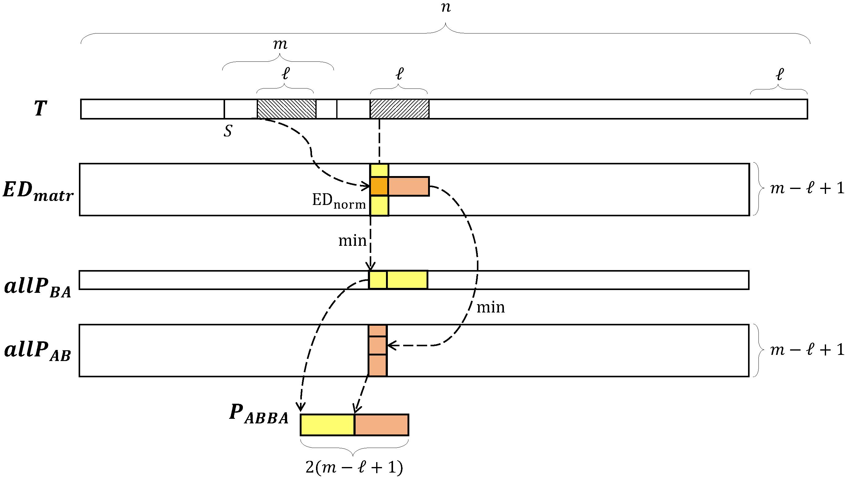
PSF employs data structures summarized in Figure 1. The computational scheme of the PSF algorithm differs from the original one as follows. The calculation of a set of MPdist-profiles (see Algorithm 1, line 2) is performed more efficiently than in the original GetAllProfiles algorithm (see Algorithm 2). Instead of one serial step at which the MPdist-profile between a segment and each subsequence of the time series is calculated, we perform a sequence of four steps, each of which is parallelized. Let us describe these steps for a fixed segment $S\in S_T^m$.

At the first step, we calculate a matrix of the ED_norm distances between the segment and each subsequence of the time series. Let us denote such a matrix as $E{D}_{matr}$:

$$E{D}_{matr}\in {\mathbb{R}}^{(m-\ell +1)\times (n-m+1)}:E{D}_{matr}(i,j)={\mathrm{ED}}_{\mathrm{norm}}(S_{i,\ell },T_{j,\ell }).$$

(21)

At the second step, for the matrix obtained at the first step, we calculate column-wise minimum values. Let us denote the resulting vector of such minima as $all{P}_{BA}$:

$$all{P}_{BA}\in {\mathbb{R}}^{n-\ell +1}:all{P}_{BA}\left(j\right)=\underset{1\le i\le m-\ell +1}{min}E{D}_{matr}(i,j).$$

(22)

At the third step, in the $E{D}_{matr}$ matrix, we calculate row-wise minimum values in an ℓ-length sliding window. Let us denote the resulting matrix as $all{P}_{AB}$:

$$all{P}_{AB}\in {\mathbb{R}}^{(m-\ell )\times (n-m+1)}:all{P}_{AB}(i,j)=\underset{j\le c\le j+\ell }{min}E{D}_{matr}(i,c).$$

(23)

Finally, at the fourth step, for each segment, we concatenate each column of the $all{P}_{AB}$ matrix and all $(m-\ell )$-length subsequences from the $all{P}_{BA}$ vector, and denote the resulting structure as $P_{ABBA}$:

$$P_{ABBA}\in {\mathbb{R}}^{2(m-\ell +1)}:P_{ABBA}\left(T_{j,\ell }\right)={\left\{all{P}_{AB}(i,j)\right\}}_{i=1}^{m-\ell +1}\odot {\left\{all{P}_{BA}\left(i\right)\right\}}_{i=j}^{m-\ell +1}.$$

(24)

In fact, at the end of this step, for a specified segment, we compute a matrix profile of the segment and each subsequence of the time series. For the final calculation of the MPdist similarity measure between the segment and a subsequence, it is necessary to sort $P_{ABBA}$ and take the k-th value of the ordered array, as defined in Equation (12).

Algorithm 4 depicts pseudo-code of the above-described steps, performed in parallel. Here, calls of the EDmatrSCAMP algorithm (line 3) provide a parallel calculation of the matrix of ED_norm distances between a specified segment and each subsequence of the time series according to Equations (8)–(10). In EDmatrSCAMP, parallel computations are based on the technique employed in the SCAMP algorithm proposed in [19]. This technique employs the following equations:

$${\overline{QT}}_{i,j}={\overline{QT}}_{i-1,j-1}+d{f}_i·d{g}_j+d{f}_j·d{g}_i,$$

(25)

$$\begin{array}{c}d{f}_0=0,d{f}_i=\frac{1}{2}(t_{i+m-1}-t_{i-1}),\\ d{g}_0=0,d{g}_i=(t_{i+m-1}-{\mu }_i)+(t_{i-1}-{\mu }_{i-1}),{\mu }_i={\displaystyle \frac{1}{m}}{\displaystyle \sum _{j=i}^{i+m}}{t}_j,\end{array}$$

(26)

$$P_{i,j}={\overline{QT}}_{i,j}·{\displaystyle \frac{1}{\Vert T_{i,m}-{\mu }_i\Vert }}·{\displaystyle \frac{1}{\Vert T_{j,m}-{\mu }_j\Vert }},$$

(27)

where $T_{i,m}-{\mu }_i={\{t_k-{\mu }_k\}}_{k=i}^{i+m-1}$, $T_{j,m}-{\mu }_j={\{t_k-{\mu }_k\}}_{k=j}^{j+m-1}$, and $\Vert ·\Vert$ denotes the Euclidean norm.

$${\mathrm{ED}}_{\mathrm{norm}}(T_{i,m},T_{j,m})=\sqrt{2m(1-P_{i,j})}.$$

(28)

Algorithm 4 ParallelGetAllProfiles (in $T,m$; out D)

1: $D\leftarrow ⌀$ 2: for $i\leftarrow 1$ to $n/m$ do 3:     $E{D}_{matr}\leftarrow$EDmatrSCAMP$(T,S_i,\ell )$ 4:     for $j\leftarrow 1$ to $n-\ell$ do            ▹ PARALLEL 5:         $all{P}_{BA}\left(j\right)\leftarrow {min}_{1\le r\le m-\ell +1}E{D}_{matr}(r,j)$ 6:     for $r\leftarrow 1$ to $m-\ell$ do           ▹ PARALLEL 7:         for $q\leftarrow 1$ to $n-m+1$ do 8:            $all{P}_{AB}(r,q)\leftarrow {min}_{q\le p\le q+\ell }E{D}_{matr}(r,p)$ 9:     $D_i\leftarrow$ParallelProfile$(all{P}_{AB},all{P}_{BA})$ 10:     $D\leftarrow D\cup D_i$ 11: return D

As opposed to its predecessor, GPU-STOMP_OPT [27], while computing the Euclidean distances, SCAMP reorders floating-point computations and replaces sliding dot product update with a centered sum-of-products formula (Equations (25)–(28)). Equation (26) precompute the terms used in the sum-of-products update formula of Equation (25), and incorporate incremental mean centering into the update. Equation (27) replaces the Euclidean distance with the Pearson Correlation that can be computed incrementally using fewer computations than the Euclidean distance, and can be converted to the z-normalized Euclidean distance in $O\left(1\right)$ by Equation (28).

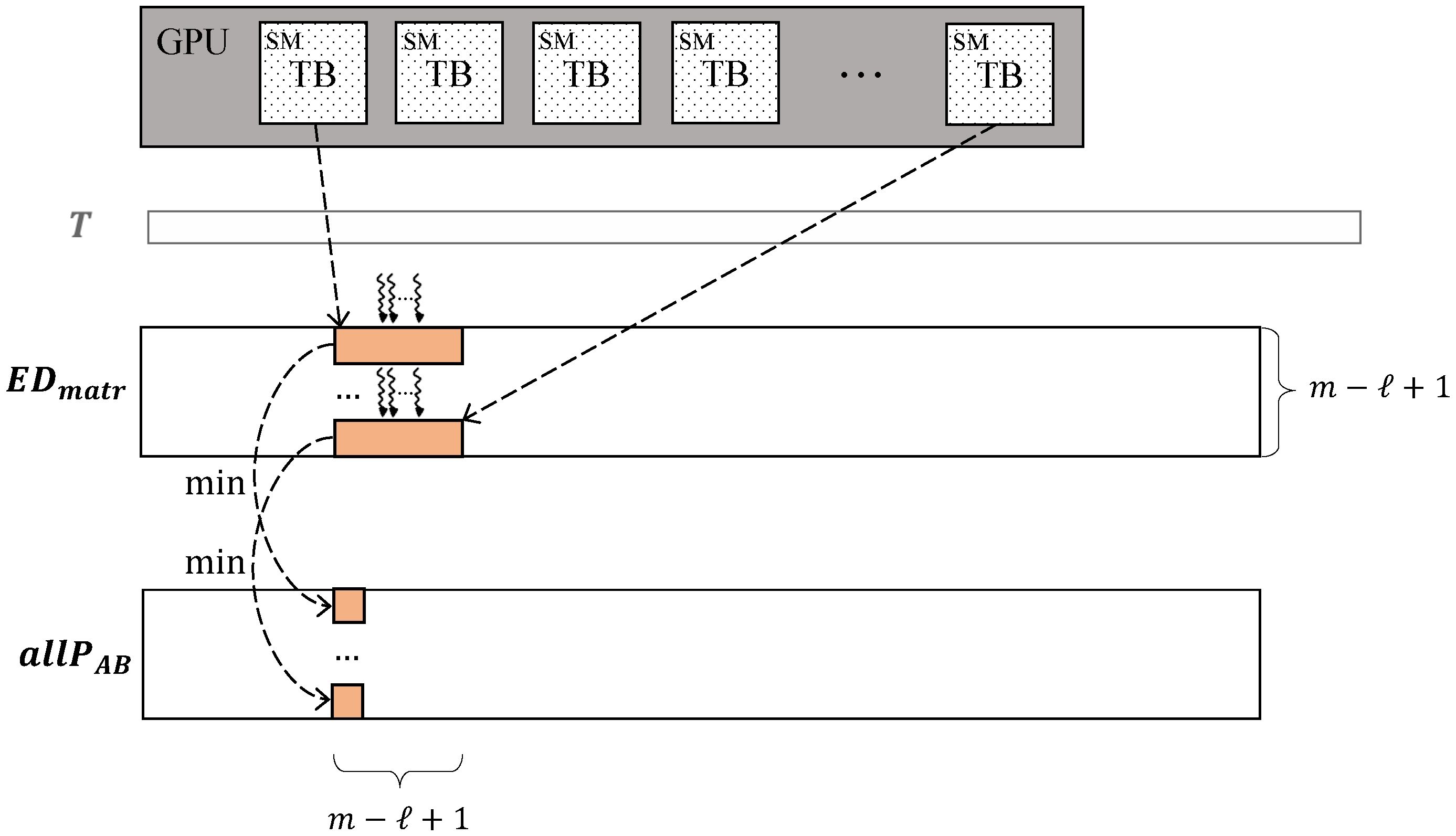
In ParallelGetAllProfiles (see Algorithm 4), lines 4–5 implement parallel calculation of the $all{P}_{BA}$ vector containing column-wise minima of the $E{D}_{matr}$ matrix according to Equation (22). The corresponding CUDA kernel is organized as follows (see Figure 2). We form a grid consisting of $n-m+1$ blocks of $m-\ell +1$ threads in each block. An $E{D}_{matr}$ column is copied from the global memory to the shared memory of each block. Finally, each block finds the minimum through the reduction operation.

Next, lines 6–8 of the algorithm implement parallel calculation of the $all{P}_{AB}$ matrix of row-wise minima in an ℓ-length sliding window of $E{D}_{matr}$ according to Equation (23). The corresponding CUDA kernel is depicted in Figure 3. We create a single block grid consisting of $m-\ell +1$ threads. Each thread calculates the minimum in an ℓ-length sliding window for one row of the matrix. The resulting matrix is stored in global memory.

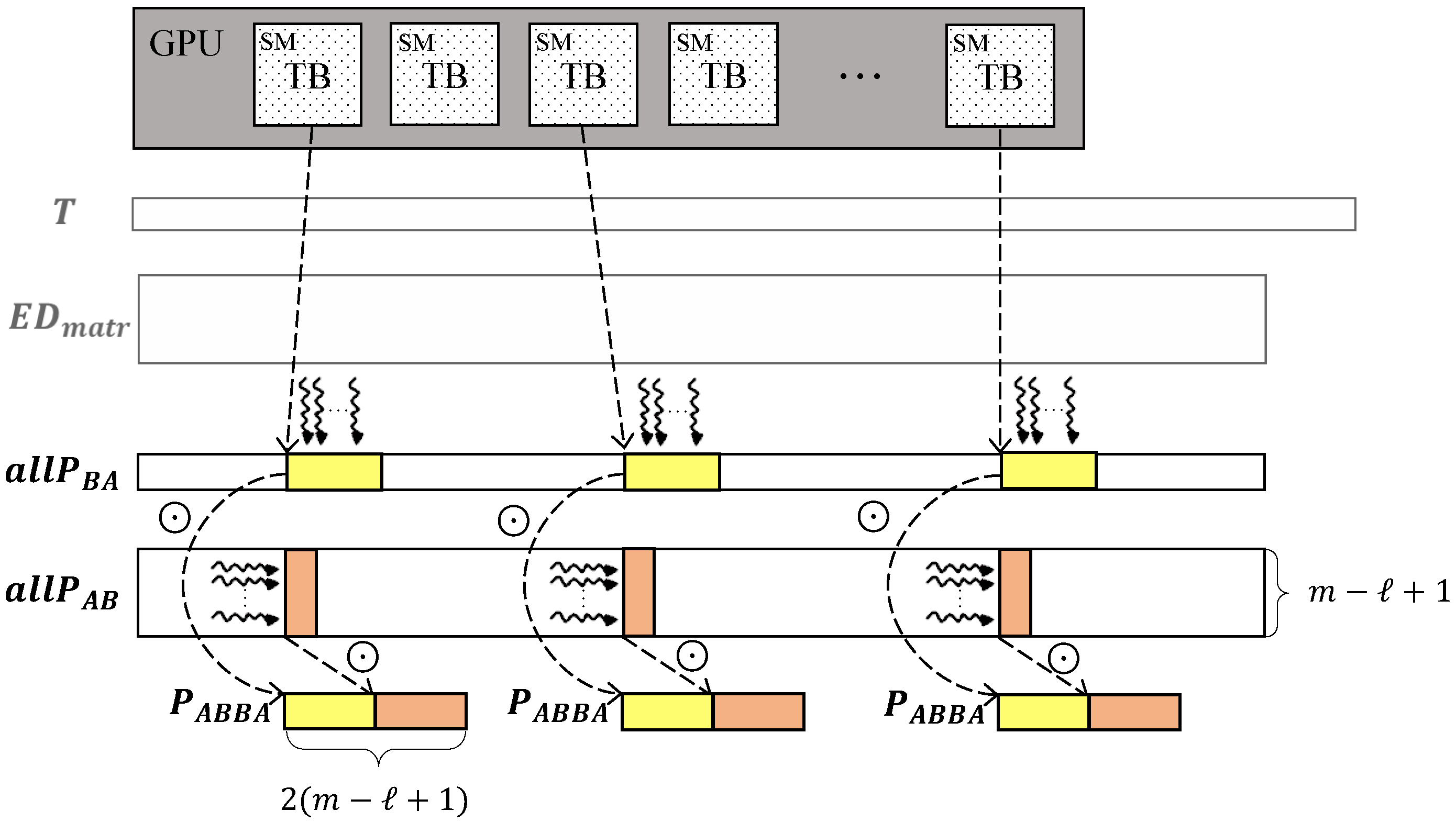
After that, calculations are continued by the ParallelProfile algorithm (see Algorithm 5). The algorithm performs according to Equation (24) through the parallel concatenation of each column of the $all{P}_{AB}$ matrix and all the $(m-\ell )$-length subsequences included in the $all{P}_{BA}$ vector.

Algorithm 5 ParallelProfile (in $all{P}_{AB},all{P}_{BA}$; out P)

1: $P\leftarrow \varnothing$; $k\leftarrow \lceil 0.1·(m-\ell )\rceil$ 2: for $i\leftarrow 1$ to $n-\ell$ do            ▹ PARALLEL 3:     $P_{ABBA}\leftarrow all{P}_{AB}\left(i\right)\odot all{P}_{BA}(i,m-\ell )$ 4:     $sorted{P}_{ABBA}\leftarrow$Sort$\left(P_{ABBA}\right)$ 5:     $P_i\leftarrow sorted{P}_{ABBA}\left(k\right)$ 6:     $P\leftarrow P\cup P_i$ 7: return P

To compute this, we employ the following CUDA kernel (see Figure 4). We create a grid consisting of $n-m+1$ blocks of $2(m-\ell +1)$ threads in each block. Each block forms the $P_{ABBA}$ matrix profile for a segment. Half of the block’s threads copy $all{P}_{AB}$ data from the global memory to the shared memory of this block, and the other half of the threads copy $all{P}_{BA}$ data from the global memory to the shared memory of this block for each column of $E{D}_{matr}$. Next, each block sorts $P_{ABBA}$ and writes its k-th element (see Equation (12)) to global memory, thus forming the MPdist-profile of the segment.

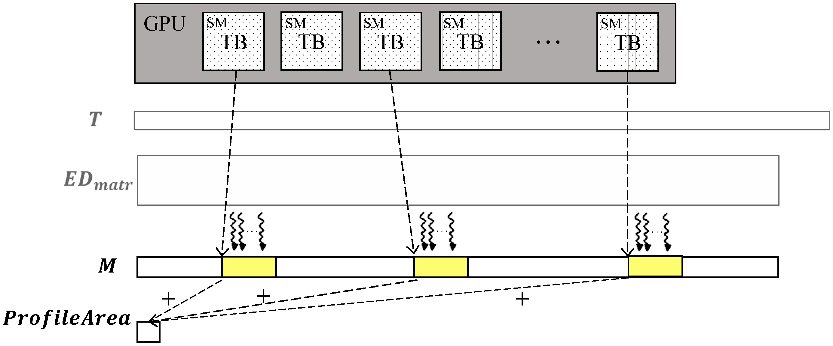
We also parallelize calculations of the area under the curve and fractions of the snippets found in the original serial algorithm (see lines 5–11 and lines 12–14 in Algorithm 1, respectively). Figure 5 depicts the respective CUDA kernels. The first kernel is a grid consisting of $n/m$ blocks of $n-m+1$ threads in each block. Each block calculates the minima of the curve. Next, elements of the curve are summed through the reduction operation. After K snippets are found, the second CUDA kernel performs as a grid consisting of K blocks of $n-m+1$ threads in each block. This grid calculates the fraction of each snippet by comparing the values of the MPdist-profiles of snippets and the curve.

5. Experimental Evaluation

To evaluate the proposed algorithm, we carried out experiments with the following objectives. First, we evaluated the performance of the PSF algorithm over time series from different subject domains in comparison with analogs. Next, we investigated how the segment length and a user-defined subsequence length (see Section 3.2) affect the performance of PSF. Finally, we also evaluated a frequently exploited idea to speed up computations in PSF through changing the Euclidean distance metric to the square thereof (see Equation (9)). We designed our experiments to be easily reproducible and have built a repository [28] that contains the algorithm’s source code and all the datasets used in this work.

Below, Section 5.1 describes the datasets and hardware platform of the experiments, and Section 5.2 presents experimental results and discussion.

5.1. The Experimental Setup

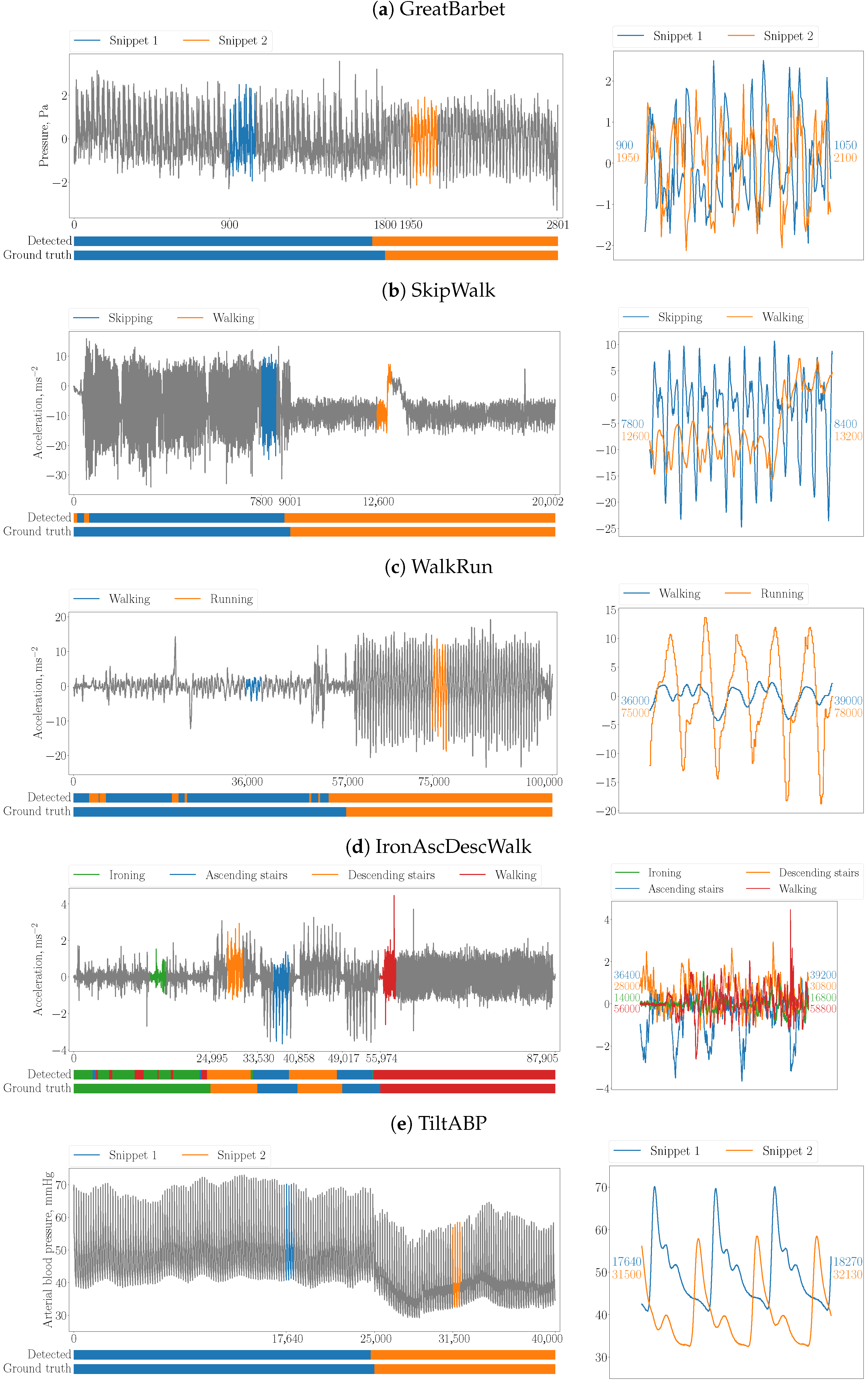
In the experiments, we employed the following time series listed in

Table 1. Time series employed in the experiments.

Time Series	Length n	Segment m	Description
GreatBarbet	2801	150	Physiological indicators of bird vital activity
WildVTrainedBird	20,002	900
SkipWalk	20,002	600	Wearable accelerometer readings during various types of human physical activity
WalkRun	100,000	240
IronAscDescWalk	87,906	2800
TiltABP	40,000	630	Human blood pressure readings  during rapid tilts
RW	100,000	in the range 250..2500	Synthetic time series

(with the given segment lengths). The GreatBarbet, WildVTrainedBird, SkipWalk, and TiltABP time series are taken from the MixedBag dataset [29], a diverse collection of one hundred time series compiled by the authors of the original serial algorithm [5] for its experimental evaluation. In MixedBag, each time series has two predefined one-time changed activities of approximately equal length. GreatBarbet and WildVTrainedBird represent physiological indicators of bird vital activity. TiltABP describes human blood pressure measurements during rapid tilts. SkipWalk illustrates the readings of a wearable accelerometer during jumping rope and walking of a human; it is an excerpt from the PAMAP dataset [30] that contains data recorded during various types of human physical activity. We also constructed the WalkRun and IronAscDescWalk time series as excerpts from PAMAP: the former reflects walking and running, and the latter shows ironing, ascending and descending stairs, and walking. Finally, RW is a synthetic time series generated according to the Random Walk model [31].

In the experiments, we compared the performance of the proposed parallel PSF algorithm, the original serial Snippet-Finder algorithm, and the parallel NaivePSF algorithm.We developed NaivePSF as a simplified version of PSF where only the most time-consuming part of snippet discovery is parallelized, namely computation of matrix profiles between segments and all subsequences according to Equations (8)–(11). We implemented such calculations on GPU through the separate calls of the SCAMP framework [19]. The rest part of calculations, namely building MPdist profiles of all segments according to Equations (11)–(14) and snippet discovery, are implemented serially on CPU. In each experiment, we ran the algorithms 10 times and took the median value as the final running time. In the experiments, for each evaluated time series, we checked that Snippet-Finder, NaivePSF, and PSF produce exactly the same snippets and resulting summarization.

For all the experiments, we set the subsequence length parameter of the MPdist measure (see Section 3.2) as $\ell =\lceil m/2\rceil$, i.e., as half of the segment length.

Table 2. Hardware platform of the experiments.

Specifications	CPU	GPU
Brand	Intel	NVIDIA
Model	Xeon Gold 6254	Tesla V100 SXM2
Cores	18	5120
Frequency, GHz	4.0	1.3
Memory, Gb	64	32
Peak performance, TFLOPS	1.2	15.7

summarizes hardware platform of the experiments. In the study, Snippet-Finder runs on CPU (on a single core). PSF and NaivePSF perform calculations mostly on GPU (Equations (8)–(20)), except for Equation (26) which is calculated on CPU.

5.2. Results and Discussion

5.2.1. Summarization

Figure 6 depicts the results of summarization for several real-world time series mentioned in Table 1.

In addition, in

Table 3. Summarization accuracy of the PSF algorithm.

Time Series	Accuracy
GreatBarbet	0.97
WildVTrainedBird	0.94
SkipWalk	0.97
WalkRun	0.91
IronAscDescWalk	0.88
TiltABP	0.99

, we show the summarization accuracy of PSF over all the real-world time series involved in experiments. By the algorithm’s accuracy, we assume a ratio of elements in the time series for which its respective activity was detected correctly to the length of the time series. We may conclude that our parallel algorithm (like the original serial one) is able to summarize a time series with accuracy pretty close to ground truth (but much faster than its predecessor, as will be shown below).

5.2.2. Performance

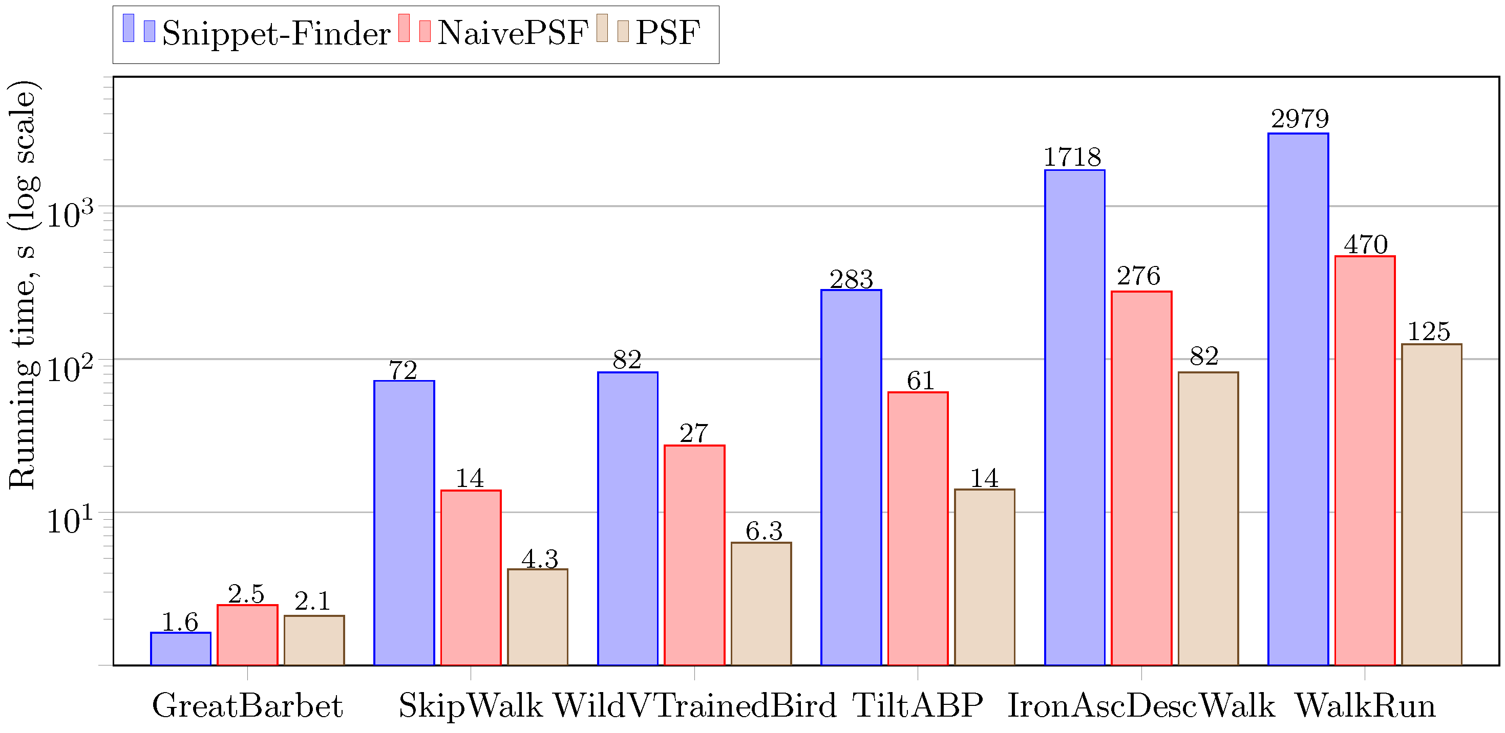
Experimental results concerning the algorithm’s performance over real-world time series are depicted in Figure 7. It can be seen that PSF, the proposed parallel algorithm, substantially (at least an order of magnitude) outruns Snippet-Finder, the original serial one, for all the time series considered in the experiments, except for GreatBarbet, the shortest one, where PSF is a bit behind Snippet-Finder. This seemingly implausible result has the following simple explanation. When a time series is relatively short (in our experiments, we found such a length as about ten thousands of elements), then the overhead of transferring data to GPU and initializing computing kernels is greater than the time spent on the actual calculations.

Similarly, for the short-length time series, PSF shows almost the same performance as NaivePSF, since the overhead of these algorithms is the same, and redundant calculations in the naive version are practically absent. For time series with a length of more than ten thousand elements, PSF is up to four times faster than NaivePSF. The advantage of the PSF algorithm is greater the longer the length of the evaluated time series, since the overhead of calculating matrix profiles between segments and subsequences of the time series becomes more significant. Additionally, the superiority of PSF over NaivePSF shows us that straightforward parallelization is not enough to achieve the highest possible performance of the snippet discovery, and the proposed data structures and parallelization scheme are crucial.

5.2.3. Impact of the Segment Length

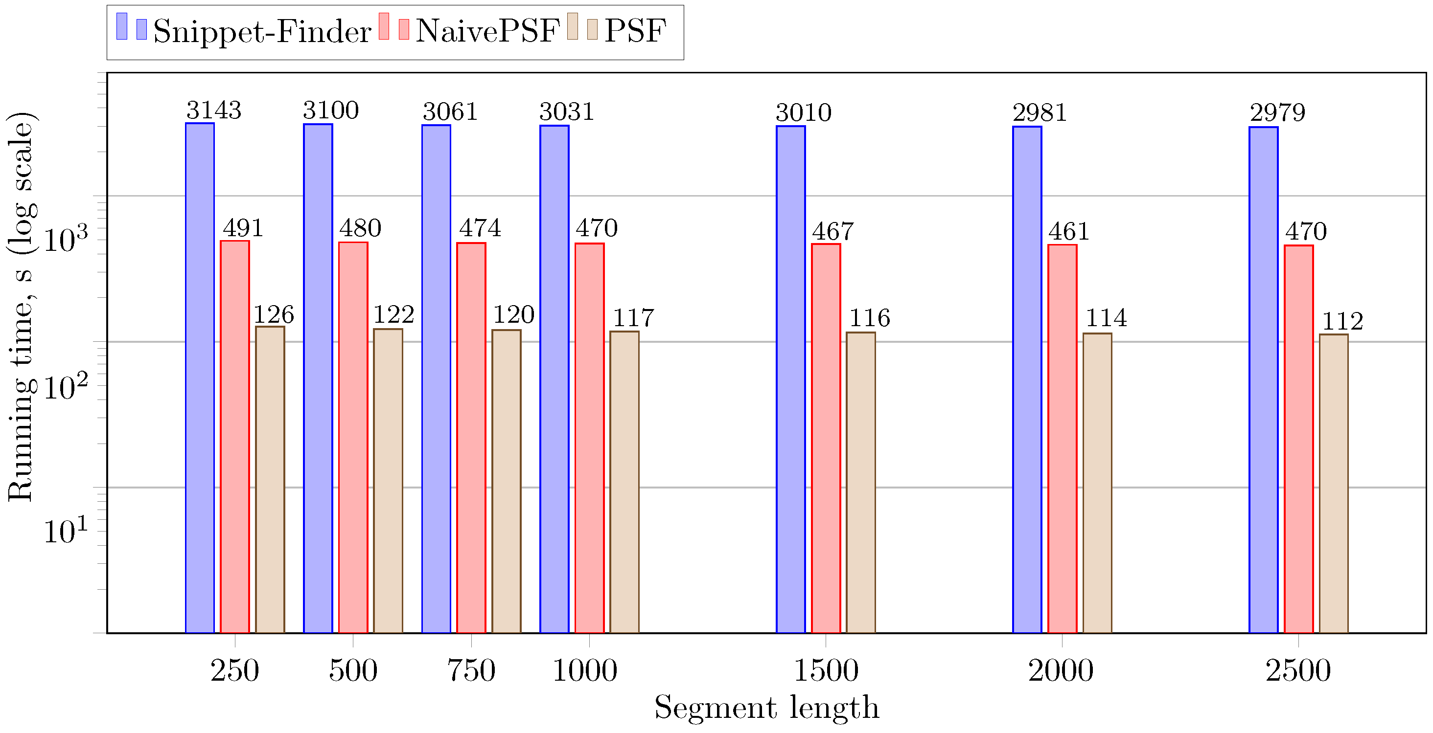
We evaluated the dependence of the parallel algorithm’s performance on the segment length (the parameter m) on the RW synthetic time series, and Figure 8 shows the experimental results. It can be seen that the proportion between the Snippet-Finder, NaivePSF, and PSF performance is retained. In addition, the algorithms’ performance increases slightly (up to two percent) as segment length increases. Since the original algorithm’s time complexity is $O(n^2·\frac{n-m}{m})$ (where n is time series length and m is segment length) [7], the overall number of operations tends to zero as the segment length increases.

5.2.4. Impact of the Subsequence Length

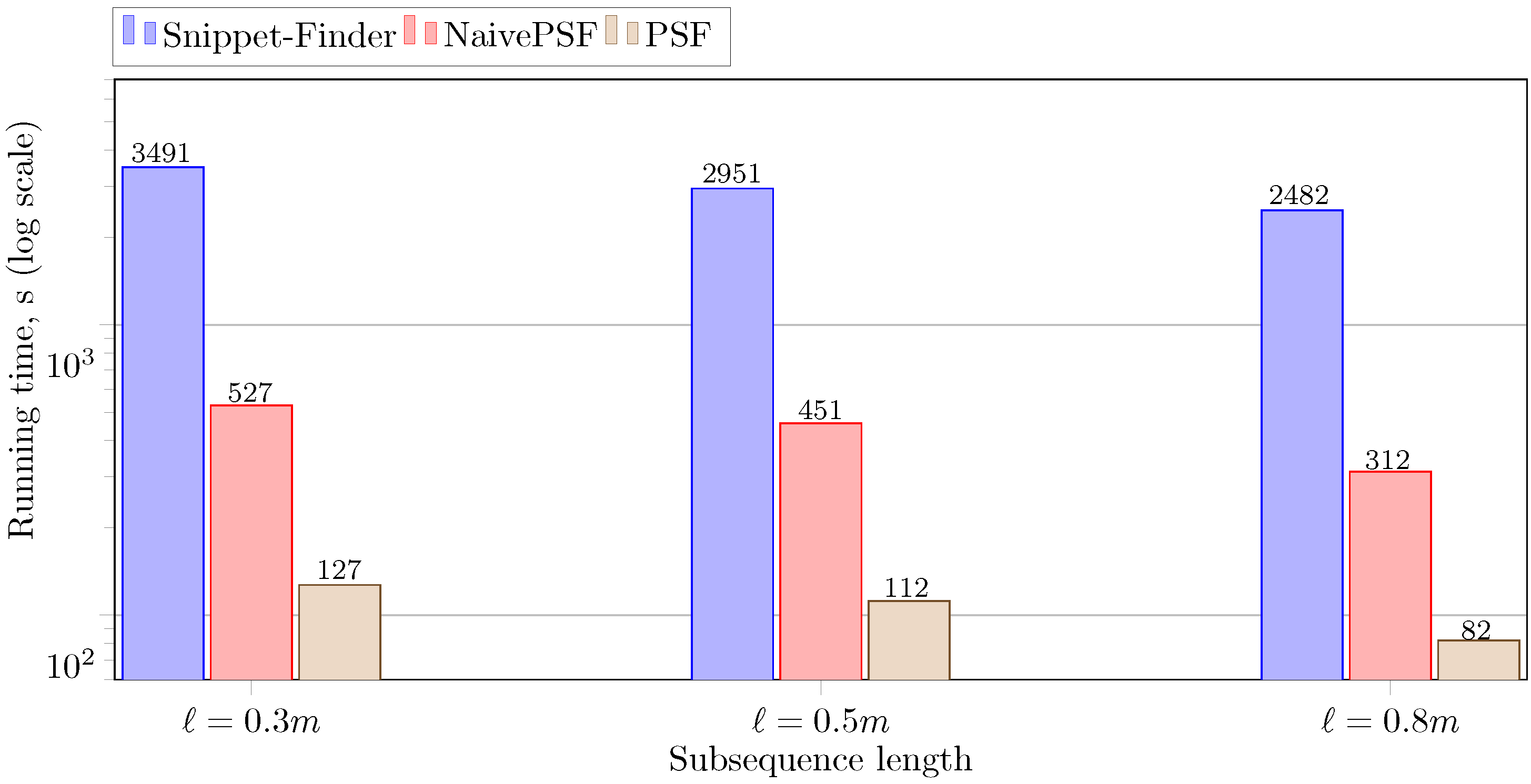
In Figure 9, we show the dependence of the parallel algorithm’s performance on the subsequence length (the parameter ℓ, see Section 3.2) for the RW synthetic time series and segment length $m=2500$. As before, the proportion between the performance of Snippet-Finder, NaivePSF, and PSF is retained. It can be seen that the greater value of the subsequence length provides us with higher algorithm’s performance. This is an expected result since greater value of the parameter ℓ results in a smaller number of rows in $E{D}_{matr}$, the matrix of distances between segments and subsequences, and, in turn, smaller size of its legacy data structures $all{P}_{BA}$, $all{P}_{AB}$, $all{P}_{BA}$, and $P_{ABBA}$ (see Equations (21)–(24) and Figure 1) all the algorithm’s calculations are based on.

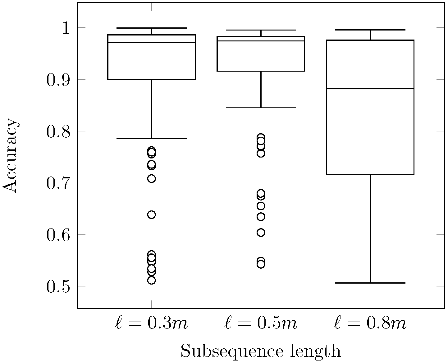
In addition, in Figure 10, we show the average accuracy of PSF over all the time series from the MixedBag dataset [29] depending on the subsequence length. From boxplots that reflect the accuracy for three typical values of the parameter ℓ, we can see that $\ell =\lceil m/2\rceil$ provides us with higher accuracy than two others. Finally, we conclude that the subsequence length, being specified as half of the segment length, provides us with the best trade-off between the performance and accuracy of PSF.

5.2.5. Applying ${\mathrm{ED}}_{\mathrm{norm}}^2$ Instead of ED_norm

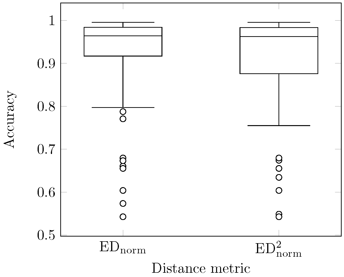
In the experiments on applying ${\mathrm{ED}}_{\mathrm{norm}}^2$ instead of ED_norm, we compared the performance and accuracy of PSF over all the time series from the MixedBag dataset [29]. Figure 11 shows two boxplots of the algorithm’s accuracy when the normalized Euclidean distance metric or the squared version thereof is employed, respectively. As can be seen, the squared distance metric can substitute the original one without a significant loss of quality. As expected, ${\mathrm{ED}}_{\mathrm{norm}}^2$ is more “strict” and demonstrates lower values of the third quartile and minimum in the cases when PSF demonstrates low accuracy. However, for these two cases, maximums, first quartiles, and medians are almost equal. At the same time, in our experiments, PSF showed up to 10 percent higher performance when the MPdist is based on the squared distance metric.

6. Conclusions

In this article, we addressed the task of accelerating the summarization of a long time series with a graphics processor. Informally, summarization can be described as discovering a small-sized set of typical patterns (subsequences) that briefly represent the long time series. The task of time series summarization arises in a wide spectrum of subject domains within analytical applications related to decision-making, modeling, planning, and so on.

A number of apparent approaches to time series summarization like motifs, shapelets, cluster centroids, and so on, have two unavoidable limitations that they either require pre-labeled training data, or cannot determine a fraction of the time series represented by the pattern found. The snippet concept recently proposed by Keogh et al. [5] overcomes the above-mentioned limitations. For a given length, a time series snippet is a subsequence that is similar to many other subsequences of the time series with respect to the MPdist similarity measure [6] based on the Euclidean distance. In addition, all the subsequences similar to the snippet can be exactly specified and counted. However, the original Snippet-Finder algorithm has a cubic time complexity concerning the lengths of the time series and snippet [7]. Thus, Snippet-Finder requires parallelization to ensure acceptable performance over very long time series. Our extensive search in recent scientific publications showed that, to the best of our knowledge, no research addresses the acceleration of time series snippet discovery with GPU or any other parallel hardware architecture.

In the article, we employed Keogh et al.’s works [5,7] as a basis and proposed a novel parallelization scheme for snippet discovery on a graphics processor. Our algorithm is called PSF (Parallel Snippet-Finder) and employs advanced data structures and a computational scheme different to the original algorithm. In PSF, we calculated MPdist-profiles more efficiently than in the original algorithm: instead of one serial step at which the MPdist-distance between a snippet and each subsequence of the time series is calculated, we performed a sequence of steps, each of which is parallelized on GPU.

We carried out an extensive experimental evaluation of PSF, employing a diverse collection of time series compiled by the authors of the original serial algorithm. For evaluation purposes, we also developed a straightforward version of PSF where only the most time-consuming part of snippet discovery (computation of distances between snippets and all subsequences) is parallelized on GPU through the separate calls of the SCAMP framework [19]. Experimental results showed that PSF outruns both the original serial algorithm and the straightforward parallel version (at least an order of magnitude and up to four times, respectively). In addition, experiments showed that PSF is well scalable with respect to its input parameters (the snippet length and subsequence length) and the similarity measure employed (based on the ordinary or squared Euclidean distance).

In further studies, we plan to extend our approach in two directions: (a) the case of a many-core CPU as an underlying hardware platform where parallelization of snippet discovery is performed through the OpenMP technology [32] instead of CUDA, and (b) the case of a large time series that cannot be entirely placed in RAM, and snippets should be found on a high-performance cluster with GPU or many-core CPU nodes.

References

- Chiu, B.Y.; Keogh, E.J.; Lonardi, S. Probabilistic discovery of time series motifs. In Proceedings of the 9th ACM SIGKDD International Conference on Knowledge Discovery and Data Mining, Washington, DC, USA, 24–27 August 2003; Getoor, L., Senator, T.E., Domingos, P.M., Faloutsos, C., Eds.; ACM: New York, NY, USA, 2003; pp. 493–498. [Google Scholar] [CrossRef]
- Mueen, A.; Keogh, E.J.; Zhu, Q.; Cash, S.; Westover, M.B. Exact Discovery of Time Series Motifs. In Proceedings of the SIAM International Conference on Data Mining, SDM 2009, Sparks, NV, USA, 30 April 30–2 May 2009; SIAM: Philadelphia, PN, USA, 2009; pp. 473–484. [Google Scholar] [CrossRef]
- Indyk, P.; Koudas, N.; Muthukrishnan, S. Identifying Representative Trends in Massive Time Series Data Sets Using Sketches. In VLDB 2000, Proceedings of 26th International Conference on Very Large Data Bases, Cairo, Egypt, 10–14 September 2000; Abbadi, A.E., Brodie, M.L., Chakravarthy, S., Dayal, U., Kamel, N., Schlageter, G., Whang, K., Eds.; Morgan Kaufmann: Burlington, MA, USA, 2000; pp. 363–372. [Google Scholar]
- Yeh, C.M.; Zhu, Y.; Ulanova, L.; Begum, N.; Ding, Y.; Dau, H.A.; Silva, D.F.; Mueen, A.; Keogh, E.J. Matrix Profile I: All Pairs Similarity Joins for Time Series: A Unifying View That Includes Motifs, Discords and Shapelets. In Proceedings of the IEEE 16th International Conference on Data Mining, ICDM 2016, Barcelona, Spain, 12–15 December 2016; Bonchi, F., Domingo-Ferrer, J., Baeza-Yates, R., Zhou, Z., Wu, X., Eds.; IEEE Computer Society: Piscataway, NJ, USA, 2016; pp. 1317–1322. [Google Scholar] [CrossRef]
- Imani, S.; Madrid, F.; Ding, W.; Crouter, S.E.; Keogh, E.J. Matrix Profile XIII: Time Series Snippets: A New Primitive for Time Series Data Mining. In Proceedings of the 2018 IEEE International Conference on Big Knowledge, ICBK 2018, Singapore, 17–18 November 2018; Wu, X., Ong, Y., Aggarwal, C.C., Chen, H., Eds.; IEEE Computer Society: Piscataway, NJ, USA, 2018; pp. 382–389. [Google Scholar] [CrossRef]
- Gharghabi, S.; Imani, S.; Bagnall, A.J.; Darvishzadeh, A.; Keogh, E.J. An ultra-fast time series distance measure to allow data mining in more complex real-world deployments. Data Min. Knowl. Discov. 2020, 34, 1104–1135. [Google Scholar] [CrossRef]
- Imani, S.; Madrid, F.; Ding, W.; Crouter, S.E.; Keogh, E.J. Introducing time series snippets: A new primitive for summarizing long time series. Data Min. Knowl. Discov. 2020, 34, 1713–1743. [Google Scholar] [CrossRef]
- Kraeva, Y.; Zymbler, M.L. Scalable Algorithm for Subsequence Similarity Search in Very Large Time Series Data on Cluster of Phi KNL. In Data Analytics and Management in Data Intensive Domains Proceedings of the 20th International Conference, DAMDID/RCDL 2018, Moscow, Russia, 9–12 October 2018; Revised Selected Papers; Manolopoulos, Y., Stupnikov, S.A., Eds.; Springer: Berlin/Heidelberg, Germany, 2018; Volume 1003, pp. 149–164. [Google Scholar] [CrossRef]
- Zymbler, M.; Kraeva, Y. Discovery of Time Series Motifs on Intel Many-Core Systems. Lobachevskii J. Math. 2019, 40, 2124–2132. [Google Scholar] [CrossRef]
- Zymbler, M.; Grents, A.; Kraeva, Y.; Kumar, S. A Parallel Approach to Discords Discovery in Massive Time Series Data. Comput. Mater. Continua 2021, 66, 1867–1878. [Google Scholar] [CrossRef]
- Zymbler, M.; Polyakov, A.; Kipnis, M. Time Series Discord Discovery on Intel Many-Core Systems. In Proceedings of the 13th International Conference, PCT 2019, Kaliningrad, Russia, 2–4 April 2019, Revised Selected Papers; Communications in Computer and Information Science; Sokolinsky, L., Zymbler, M., Eds.; Springer: Cham, Switzerland, 2019; Volume 1063, pp. 168–182. [Google Scholar] [CrossRef]
- Zymbler, M.; Kraeva, Y. Parallel Algorithm for Time Series Motif Discovery on Graphic Processor. Bull. South Ural State Univ. Ser. Comput. Math. Softw. Eng. 2020, 9, 17–34. (In Russian) [Google Scholar] [CrossRef]
- Zymbler, M.; Ivanova, E. Matrix profile-based approach to industrial sensor data analysis inside RDBMS. Mathematics 2021, 9, 2146. [Google Scholar] [CrossRef]
- Keogh, E.J.; Lin, J. Clustering of time-series subsequences is meaningless: Implications for previous and future research. Knowl. Inf. Syst. 2005, 8, 154–177. [Google Scholar] [CrossRef]
- Narang, A.; Bhattacherjee, S. Parallel Exact Time Series Motif Discovery. In Lecture Notes in Computer Science, Proceedings of the 16th International Euro-Par Conference, Ischia, Italy, 31 August–3 September 2010; D’Ambra, P., Guarracino, M.R., Talia, D., Eds.; Springer: Berlin/Heidelberg, Germany, 2010; Volume 6272, pp. 304–315. [Google Scholar] [CrossRef]
- Fernandez, I.; Villegas, A.; Gutiérrez, E.; Plata, O.G. Accelerating time series motif discovery in the Intel Xeon Phi KNL processor. J. Supercomput. 2019, 75, 7053–7075. [Google Scholar] [CrossRef] [Green Version]
- Zhu, B.; Jiang, Y.; Gu, M.; Deng, Y. A GPU Acceleration Framework for Motif and Discord Based Pattern Mining. IEEE Trans. Parallel Distrib. Syst. 2021, 32, 1987–2004. [Google Scholar] [CrossRef]
- Kaufman, L.; Rousseeuw, P.J. Finding Groups in Data: An Introduction to Cluster Analysis; John Wiley: Berlin/Heidelberg, Germany, 1990. [Google Scholar] [CrossRef]
- Zimmerman, Z.; Kamgar, K.; Senobari, N.S.; Crites, B.; Funning, G.J.; Brisk, P.; Keogh, E.J. Matrix Profile XIV: Scaling Time Series Motif Discovery with GPUs to Break a Quintillion Pairwise Comparisons a Day and Beyond. In Proceedings of the ACM Symposium on Cloud Computing, SoCC 2019, Santa Cruz, CA, USA, 20–23 November 2019; ACM: New York, NY, USA, 2019; pp. 74–86. [Google Scholar] [CrossRef]
- Hendryx, E.P.; Rivière, B.M.; Sorensen, D.C.; Rusin, C.G. Finding representative electrocardiogram beat morphologies with CUR. J. Biomed. Inform. 2018, 77, 97–110. [Google Scholar] [CrossRef] [PubMed]
- Lu, L.; Zhang, H. Automated extraction of music snippets. In Proceedings of the 11th ACM International Conference on Multimedia, Berkeley, CA, USA, 2–8 November 2003; Rowe, L.A., Vin, H.M., Plagemann, T., Shenoy, P.J., Smith, J.R., Eds.; ACM: New York, NY, USA, 2003; pp. 140–147. [Google Scholar] [CrossRef]
- Luqian, S.; Yuyuan, Z. Human Activity Recognition Using Time Series Pattern Recognition Model-Based on tsfresh Features. In Proceedings of the 17th International Wireless Communications and Mobile Computing, IWCMC 2021, Harbin, China, 28 June–2 July 2021; IEEE: Piscataway, NJ, USA, 2021; pp. 1035–1040. [Google Scholar] [CrossRef]
- Bascol, K.; Emonet, R.; Fromont, É.; Odobez, J. Unsupervised Interpretable Pattern Discovery in Time Series Using Autoencoders. In Structural, Syntactic, and Statistical Pattern Recognition—Joint IAPR International Workshop, S+SSPR 2016, Mérida, Mexico, 29 November–2 December 2016, Proceedings; Lecture Notes in Computer Science; Robles-Kelly, A., Loog, M., Biggio, B., Escolano, F., Wilson, R.C., Eds.; Springer: Cham, Switzerland, 2016; Volume 10029, pp. 427–438. [Google Scholar] [CrossRef]
- Noering, F.K.; Schröder, Y.; Jonas, K.; Klawonn, F. Pattern discovery in time series using autoencoder in comparison to nonlearning approaches. Integr. Comput. Aided Eng. 2021, 28, 237–256. [Google Scholar] [CrossRef]
- Lloyd, S.P. Least squares quantization in PCM. IEEE Trans. Inf. Theory 1982, 28, 129–136. [Google Scholar] [CrossRef] [Green Version]
- Kirk, D.B. NVIDIA CUDA software and GPU parallel computing architecture. In Proceedings of the 6th International Symposium on Memory Management, ISMM 2007, Montreal, QC, Canada, 21–22 October 2007; Morrisett, G., Sagiv, M., Eds.; ACM: New York, NY, USA, 2007; pp. 103–104. [Google Scholar] [CrossRef]
- Zhu, Y.; Zimmerman, Z.; Senobari, N.S.; Yeh, C.M.; Funning, G.J.; Mueen, A.; Brisk, P.; Keogh, E.J. Exploiting a novel algorithm and GPUs to break the ten quadrillion pairwise comparisons barrier for time series motifs and joins. Knowl. Inf. Syst. 2018, 54, 203–236. [Google Scholar] [CrossRef] [Green Version]
- Goglachev, A.; Zymbler, M. Parallel Snippet Finder Algorithm for CUDA. 2022. Available online: https://github.com/goglachevai/PSF (accessed on 14 May 2022).
- Imani, S.; Madrid, F.; Ding, W.; Crouter, S.E.; Keogh, E.J. Snippet-Finder Supporting Website. 2021. Available online: https://sites.google.com/site/snippetfinderinfo/ (accessed on 30 September 2021).
- Reiss, A.; Stricker, D. Introducing a New Benchmarked Dataset for Activity Monitoring. In Proceedings of the 16th International Symposium on Wearable Computers, ISWC 2012, Newcastle, UK, 18–22 June 2012; IEEE Computer Society: Piscataway, NJ, USA, 2012; pp. 108–109. [Google Scholar] [CrossRef]
- Pearson, K. The problem of the random walk. Nature 1905, 72, 294. [Google Scholar] [CrossRef]
- De Supinski, B.R.; Scogland, T.R.W.; Duran, A.; Klemm, M.; Bellido, S.M.; Olivier, S.L.; Terboven, C.; Mattson, T.G. The Ongoing Evolution of OpenMP. Proc. IEEE 2018, 106, 2004–2019. [Google Scholar] [CrossRef]
Figure 1.
Data structures of the PSF algorithm.
Figure 2.
CUDA kernel to compute (hereinafter in figures: SM—streaming multiprocessor, TB—thread block).
Figure 3.
CUDA kernel to compute .
Figure 4.
Figure 5.
CUDA kernels to compute area under the curve and fractions.
Figure 6.
Summarization of time series with the PSF algorithm (left: top—time series where snippets are colored, bottom—ground truth labeling and this one detected through the snippets; right: the snippets found including their start and end indexes).
Figure 7.
Performance of the PSF algorithm.
Figure 8.
Performance of the PSF algorithm depending on the segment length.
Figure 9.
Performance of the PSF algorithm depending on the subsequence length.
Figure 10.
Accuracy of the PSF algorithm depending on the subsequence length.
Figure 11.
Accuracy of the PSF algorithm depending on the distance metric.