GATSMOTE: Improving Imbalanced Node Classification on Graphs via Attention and Homophily

Abstract

In recent decades, non-invasive neuroimaging techniques and graph theories have enabled a better understanding of the structural patterns of the human brain at a macroscopic level. As one of the most widely used non-invasive techniques, an electroencephalogram (EEG) may collect non-neuronal signals from “bad channels”. Automatically detecting these bad channels represents an imbalanced classification task; research on the topic is rather limited. Because the human brain can be naturally modeled as a complex graph network based on its structural and functional characteristics, we seek to extend previous imbalanced node classification techniques to the bad-channel detection task. We specifically propose a novel edge generator considering the prominent small-world organization of the human brain network. We leverage the attention mechanism to adaptively calculate the weighted edge connections between each node and its neighboring nodes. Moreover, we follow the homophily assumption in graph theory to add edges between similar nodes. Adding new edges between nodes sharing identical labels shortens the path length, thus facilitating low-cost information messaging.

1. Introduction

Brain science is an area of great academic interest but features serious imbalance problems, such as “bad channels” during electroencephalographic recordings [1], artifact detection [2], and seizure onset zone detection [3]. The channels showing aberrant signals recorded via electroencephalogram (EEG) are classically identified as “bad channels” [1]. These aberrant signals arise from disconnected/broken electrodes or other parasitic electrical activity recorded by the EEG amplifier. In practice, users must browse through all channels to visually identify bad ones. This practice suffers from several limitations. First, the process of discerning bad channels requires a certain degree of expertise in brain science. Second, the task is arduous; it requires extensive processing time, especially when dealing with large datasets. Third, its reproducibility is poor due to variability within and between experts. It is thus important to propose methodological approaches to identify bad channels, particularly for large datasets. The number of bad channels additionally tends to be much smaller than the number of channels that work well. The datasets on EEG recording channels also possess imbalanced class distributions. As such, any methodology suggested to identify bad channels should simultaneously address the class imbalance problem.

Datasets with imbalanced class distributions are not limited to brain science. They exist in many real-life scenarios, such as fraud detection [4], network intrusion detection [5], and so on. The relative ubiquity of the class imbalance problem has inspired an array of strategies to solve it. Conventional methods can be roughly divided into two main categories: algorithm-level methods and data-level methods [6,7]. Algorithm-level solutions involve modifying learners to increase bias toward the minority class; data-level solutions entail re-sampling data to balance the class distributions. Compared with algorithm-level methods, data-level methods are more universally used because they can be flexibly adapted with novel techniques. Oversampling methods represent one of the most common data-level approaches. These methods generate synthetic samples to balance class distributions [8]. However, directly applying traditional oversampling methods to brain science, as in the case of EEG bad-channel detection, will return suboptimal solutions due to the data’s unique characteristics.

The topological properties of EEG networks can be structurally characterized as an undirected graph network [9], where EEG sensors serve as nodes and a neuroline between any two sensors represents an edge between nodes. EEG signals from different channels can also be modeled as a graph network based on the brain’s functional connectivity [10]. The signals of each EEG channel record distinct anatomical regions, serving as graph nodes. The raw feature vector of each signal represents the feature vector of each node. The edge connections between nodes can be obtained based on the presence or strength of two anatomical regions; that is, the edges between nodes can be computed using the EEG signals for each brain region (e.g., via Pearson correlation analysis of signals) followed by a manually set threshold [11]. As mentioned, the number of well-functioning channels exceeds the number of bad channels, hence the existence of class-imbalanced nodes in the EEG graph network. Although oversampling methods can alleviate the class imbalance problem, directly applying oversampling methods in EEG to generate synthetic samples comes with several difficulties. The brain network comprises a collection of nodes and edges. A principal challenge thus involves discerning the connections between synthetic samples and the original graph.

Several efforts have been made to rectify the class imbalance problem in graph data. GraphSMOTE [12] is a highly representative work using graph neural networks (GNNs) for imbalanced node classification. GraphSMOTE generates synthetic samples and trains a weight matrix based on the edge connections between nodes in the original graph. Yet it only considers the connectivity between nodes based on their feature similarity while potentially ignoring important information about the graph’s topology. In addition, existing research using GNNs for imbalanced node classification may achieve suboptimal performance in brain science due to neglecting the small-world architecture of the brain science network. Small-world architecture features a high clustering coefficient and short path length [13,14]. The clustering coefficient measures the extent of local cliquishness with a high value indicating that a node is more likely to connect with neighboring nodes. The path length measures the capacity for information integration, with a low value reflecting that information can be transferred globally through a small number of edges.

In addressing the brain network’s small-world architecture, we propose GATSMOTE, which is a novel edge generator that utilizes the attention mechanism and homophily in graph theory to connect synthetic samples to the original graph. Our designed edge generator corresponds to the two aforementioned attributes of the brain network: high local cliquishness and short path length. First, we adopt the attention mechanism to learn relation information between each node and its neighboring nodes. Attention coefficients are only calculated within a given neighborhood; denoting these coefficients as weighted edge connections helps our edge generator preserve more locality information. Second, we propose two hypotheses following the homophily assumption in graph theory to improve our edge generator’s fit to the two noted characteristics of the brain network. Homophily assumes that nodes tend to connect with similar nodes [15]. We define two metrics to measure the similarity between nodes: the similarity between their feature vectors and the similarity between labels. Then, we suggest adding relational edges between similar nodes. Adding edges between nodes with identical labels also shortens the path length to facilitate information transmission.

In summary, our contributions are as follows:

• Previous studies have emphasized the importance of connecting synthetic nodes to the original graph; however, the small-world architecture of the brain network was ignored. In this paper, to preserve the high local cliquishness of the brain network and the local graph topology, we calculate the weighted edge connections based on the attention mechanism (i.e., we only calculate the attention coefficient of each node among its neighboring nodes).
• We follow the homophily assumption in graph theory in that nodes tend to connect with similar nodes. We propose two hypotheses related to adding edges between nodes with a highly similar feature space and label space.
• We conduct extensive experiments involving an imbalanced node classification task. Experimental results demonstrate that our proposed framework can achieve state-of-the-art performance on imbalanced node classification.

2. Related Work and Methods

2.1. Class Imbalance Problem

Generally speaking, two types of techniques are available to solve the class imbalance problem: algorithm-level and data-level approaches. Algorithm-level methods modify classifiers by adjusting the specific mechanisms that would fail in the imbalanced setting [16,17]. However, the performance of modified classifiers is restricted to the chosen classifier. If the selected classifier performs poorly in some scenarios, the performance of modified classifiers is limited in kind [18].

Data-level methods, by contrast, are more universal in that they can be integrated with any classifier [19,20]. Data-level solutions focus on either undersampling or oversampling. Undersampling methods remove the majority instances; however, doing so can lead to information loss [8]. Oversampling methods increase the number of minority classes to balance the class distributions. SMOTE [8] is the most representative work, and the utilized interpolation method has been widely adapted to other oversampling methods. Mathematically, given an existing sample $\mathbf{x}\in {\mathbb{R}}^f$, the interpolation method chooses one candidate point ${\mathbf{x}}^{\prime }$ (i.e., one of ${\mathbf{x}}^{\prime }$s k-nearest neighbors) and then generates a synthetic sample $\mathbf{s}$ as follows:

$$\mathbf{s}=\mathbf{x}+\gamma ·({\mathbf{x}}^{\prime }-\mathbf{x}),$$

(1)

where $\gamma$ is a constant vector.

2.2. GNNs for Imbalanced Node Classification

First, we introduce GNNs for node classification tasks. Suppose there is a given graph $\mathbf{G}=\{\mathbf{V},\mathbf{A},\mathbf{X}\}$, where $\mathbf{V}=\{{\mathbf{v}}_1,\cdots ,{\mathbf{v}}_n\}$ is a set of n nodes; $\mathbf{A}\in {\mathbb{R}}^{n\times n}$ is an adjacency matrix; $X\in {\mathbb{R}}^{n\times d}$ denotes the feature matrix, and d is the number of features per node. In the node classification task, we denote ${\mathbf{Y}}_L\in {\mathbb{R}}^{n\times C}$ as the label information for nodes in $\mathbf{G}$, where C is the number of classes.

In this paper, we consider a Message Passing Neural Network (MPNN) which propagates node information from one node to another along edges [21]. MPNN runs M-step message passing iterations to propagate node information. The k-th message passing function ${\mathbf{h}}_v^k$ is defined as:

$${\mathbf{h}}_v^m=F_m({\mathbf{h}}_v^{m-1},\sum _{u\in N_v}{f}_m({\mathbf{h}}_v^{m-1},{\mathbf{h}}_u^{m-1},E_{vu})),$$

(2)

where ${\mathbf{h}}_v^0={\mathbf{x}}_v$, which is the input feature vector of node v; $F_m(·)$ and $f_m(·)$ are functions with learnable parameters. $E_{vu}$ is the edge connection between node v and u, and it determines the neighbors of each node $N_v$.

As the number of $N_v$ varies substantially, it is inefficient to utilize all the neighbors of each node. GraphSage [22] accordingly samples a fixed number of each node’s neighbors and then transmits node information as follows:

$${\mathbf{h}}_v^m=\sigma (W^m·f_m({\mathbf{h}}_v^{m-1},\{{\mathbf{h}}_u^{m-1},\forall u\in N_v\})),$$

(3)

where ${\mathbf{h}}_v^0={\mathbf{x}}_v$, $N_v$ represents the sampled neighbors of node v, and $f_m(·)$ is an aggregation function, such as the mean, sum or max.

Equation (3) shows that each node neighbor contributes equally to information transmission. Different from GraphSage, GAT [23] proposes the attention mechanism to learn the importance of the neighbor node u to node v as follows:

$${\mathbf{h}}_v^m=\sigma \left(\sum _{u\in N_v}{\alpha }_{vu}^m{\mathbf{W}}^m{\mathbf{h}}_u^{m-1}\right),$$

(4)

where ${\mathbf{h}}_v^0={\mathbf{x}}_v$, ${\mathbf{W}}^m$ is the learnable weight matrix, and the coefficient ${\alpha }^m$ computed by the attention mechanism is defined as:

$${\alpha }_{vu}^m=\frac{exp\left(LeakyReLU\left({\mathbf{a}}^T[{\mathbf{W}}^m{\mathbf{h}}_v^{m-1}\parallel {\mathbf{W}}^m{\mathbf{h}}_u^{m-1}]\right)\right)}{{\sum }_{u\in N_v}exp\left(LeakyReLU\left({\mathbf{a}}^T[{\mathbf{W}}^m{\mathbf{h}}_v^{m-1}\parallel {\mathbf{W}}^m{\mathbf{h}}_u^{m-1}]\right)\right)},$$

(5)

where ${\mathbf{a}}^T$ represents the transportation of the weight vector $\mathbf{a}$, and ‖ is the concatenation operation. To further increase the expressive capability, GAT [23] proposes multi-head attention thusly:

$${\mathbf{h}}_v^m{= \parallel }_{k=1}^K\sigma (\sum _{u\in N_v}{\alpha }_{vu}^{km}{\mathbf{W}}^{km}{\mathbf{h}}_u^{k(m-1)}),$$

(6)

where ${\alpha }^{km}$ is the attention coefficient computed by the k-th attention mechanism at the m-th message passing iteration and ${\mathbf{W}}^{km}$ is the corresponding learnable weight matrix.

Several recent works have addressed imbalanced node classification on graphs via GNNs. GraphSMOTE [12] is one example: it generates synthetic nodes in the embedding space and trains an edge generator to model the relation information between nodes. First, it adopts one GraphSage block as the feature extractor to decrease the feature dimensions of each node as follows:

$${\mathbf{h}}_v^1=\sigma ({\mathbf{W}}^1·CONCAT({\mathbf{x}}_v,\{{\mathbf{x}}_u,\forall u\in N_v\})),$$

where ${\mathbf{W}}^1$ is the weight parameter, $\mathbf{x}\in {\mathbb{R}}^d$ is the raw feature vector, and $\mathbf{h}\in {\mathbb{R}}^{\tilde{d}}$ is the embedding feature vector. This equation follows Equation (3), changing $m=1$, such that the aggregation function becomes $f_m=CONCAT(·)$. After feature extraction, GraphSMOTE [12] adopts the idea of SMOTE [8] to perform interpolation in the embedding feature space $\mathbf{H}\in {\mathbb{R}}^{n\times \tilde{d}}$. As stated in Section 2.1, the first step of interpolation is to find a candidate point. GraphSMOTE denotes the nearest neighbor which shares the same class label of node v as the candidate point $nn\left(v\right)$ for node v. After that, GraphSMOTE follows the interpolation equation (Equation (1)) to generate synthetic nodes ${\mathbf{V}}^{\prime }$.

Because the synthetic nodes are isolated from the original graph, GraphSMOTE trains an edge generator to capture the relation information as follows:

$$E_{vu}=softmax\left(\sigma ({\mathbf{h}}_v^1·\mathbf{S}·{\mathbf{h}}_u^1)\right),L_{edge}={\parallel \mathbf{E}-\mathbf{A}\parallel }^2,$$

where $E_{vu}$ is the reconstructed relation information between nodes v and u of the original graph, and $\mathbf{S}\in {\mathbb{R}}^{n\times n}$ is the parameter matrix optimized by the mean squared error-based loss function. Moreover, $\mathbf{S}$ preserves the relation information of the whole original graph based on each node’s embedding vector ${\mathbf{h}}^1$ and the adjacency matrix $\mathbf{A}$. The local topology of graph data is ignored, and the long path length between the original nodes is preserved.

3. Methodology

3.1. Problem Statement

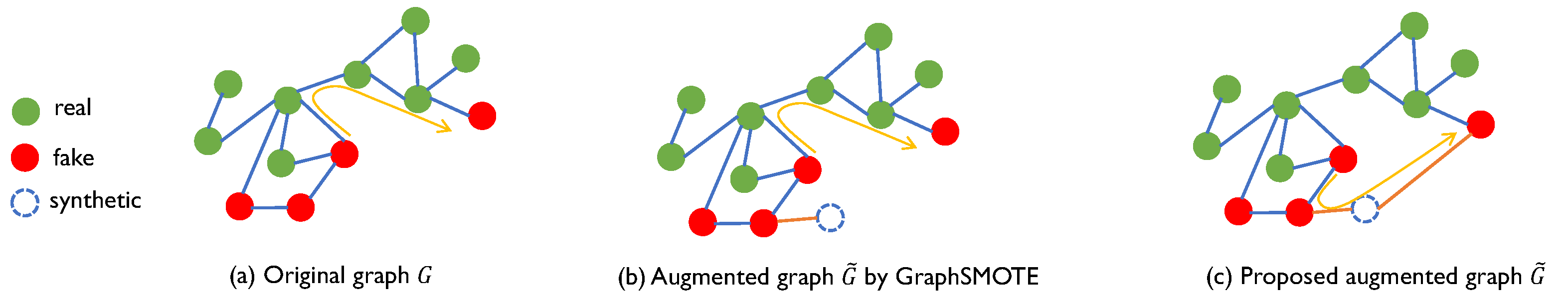
Recall that in Section 2.2, we introduce GNNs for node classification tasks. Given a graph $\mathbf{G}=\{\mathbf{V},\mathbf{A},\mathbf{X}\}$, where $\mathbf{V}$ is a set of n nodes; $\mathbf{A}\in {\mathbb{R}}^{n\times n}$ is an adjacency matrix, and $\mathbf{X}\in {\mathbb{R}}^{n\times d}$ denotes a feature matrix: let ${\mathbf{Y}}_L\in {\mathbb{R}}^{n\times C}$ denote the label information. The aim of a typical node classification task is to learn a node classifier f; that is, $f(\mathbf{V},\mathbf{A},\mathbf{X})\to {\mathbf{Y}}_L$. However, if we assume that the C classes have a varied number of nodes, the typical node classifier f will perform poorly. Following GraphSMOTE [12], we define the class imbalance ratio (IR) as the ratio of the smallest minority class to the largest majority class in the graph. As shown in Figure 1a, the original graph has the class imbalance problem. The number of fake users is obviously smaller than the number of real users.

If the IR is relatively small, we need to generate synthetic nodes ${\mathbf{V}}^{\prime }$ with a feature matrix ${\mathbf{X}}^{\prime }$ to balance the class distribution. The label information ${\mathbf{Y}}^{\prime }$ of synthetic nodes is produced simultaneously during node generation. We then need to connect the synthetic nodes to the original graph G. Therefore, it is necessary to propose an edge generator to model the edges for ${\mathbf{V}}^{\prime }$, denoted as $\mathbf{E}\in {[0,1]}^{|{\mathbf{V}}^{\prime }|\times (|{\mathbf{V}}^{\prime }|+|\mathbf{V}\left|\right)}$. We ultimately obtain an augmented graph $\tilde{\mathbf{G}}=\{\tilde{\mathbf{V}},\tilde{\mathbf{A}},\tilde{\mathbf{X}}\}$ and new label information $\tilde{\mathbf{Y}}$, where $\tilde{\mathbf{V}}=\mathbf{V}\cup {\mathbf{V}}^{\prime }$, $\tilde{\mathbf{X}}=\mathbf{X}\cup {\mathbf{X}}^{\prime }$, $\tilde{\mathbf{A}}=\mathbf{A}\cup \mathbf{E}$, and ${\tilde{\mathbf{Y}}}_L={\mathbf{Y}}_L\cup {\mathbf{Y}}_L^{\prime }$. Formally, the imbalanced node classification in this paper is defined as:

Definition 1.

Given an augmented graph $\tilde{\mathbf{G}}$ and augmented label information ${\tilde{\mathbf{Y}}}_L$, we aim to train a node classifier f that can perform classification well on both the majority and minority classes and can be used to predict the labels ${\mathbf{Y}}_U$ of unlabeled nodes. The node classifier f is defined as

$$f(\tilde{\mathbf{V}},\tilde{\mathbf{A}},\tilde{\mathbf{X}})\to {\tilde{\mathbf{Y}}}_L$$

(7)

3.2. Edge Generator

Provided that we have followed the interpolation method in GraphSMOTE [12] to generate synthetic nodes ${\mathbf{V}}^{\prime }$, these nodes are still isolated from the original graph $\mathbf{G}$. Thus, we need to train an edge generator to model the edge connections. As stated in Section 2.2, if GraphSMOTE [12] were to train a weight matrix based on the entire original graph, then the local graph information would be neglected (Figure 1b). In other words, it is poorly suited to the brain network’s high locality. In reference to Equation (5), the attention coefficients ${\alpha }_{v,u}$ are only calculated for nodes $u\in N_v$, where $N_v$ is the node v’s neighboring node set. The attention mechanism therefore corresponds to the characteristics of the brain network: the nodes are more likely to connect with their neighboring nodes [13]. Moreover, $N_v$ contains the first-order neighbors of node v and node v itself. Using this method to calculate attention coefficients will preserve the structural information of the graph network.

From the above two perspectives, we adopt the attention mechanism in graph attention networks (GATs) [23] to calculate the values of weighted edge connections. At the t-th step message passing iteration, we have the embedding vectors of the augmented nodes ${\tilde{\mathbf{H}}}^t\in {\mathbb{R}}^{\tilde{d}}$, where ${\tilde{\mathbf{H}}}^0$ is the augmented set of nodes in the original graph and the synthetic nodes generated via SMOTE [8]. For the k-th attention mechanism, we follow GAT [23]: we use a linear transformation, parameterized by a weight matrix ${\mathbf{W}}^{tk}\in {\mathbb{R}}^{\tilde{d}\times \tilde{d}}$, and a single-layer feedforward neural network, parameterized by a weight vector ${\mathbf{a}}^{tk}\in {\mathbb{R}}^{2\tilde{d}}$ to calculate the attention coefficients $e^{tk}$. Mathematically, the attention coefficients are expressed as:

$$e_{vu}^{tk}=exp\left(LeakyReLU\left({\left({\mathbf{a}}^{tk}\right)}^{\top }[{\mathbf{W}}^{tk}{\tilde{\mathbf{h}}}_v^t\parallel {\mathbf{W}}^{tk}{\tilde{\mathbf{h}}}_u^t]\right)\right),$$

(8)

where $u\in N_v$, ${(·)}^{\top }$ represents transportation, and ‖ represents the concatenation operation.

Each $e_{vu}^{tk}$ can represent the weighted connections between node v and u at the t-th step message passing iteration and the k-th attention mechanism. However, we adopt multi-head attention to stabilize the learning process; this technique generates multiple values for the weighted edge connections between nodes. We further propose a linear layer to fuse the attention coefficients from each attention mechanism as follows:

$${\mathbf{E}}^t=\frac{1}{{exp}^{-{\sum }_k{e}^{tk}·\gamma +\beta }+1},$$

(9)

where ${\mathbf{E}}^t\in {[0,1]}^{|{\mathbf{V}}^{\prime }|\times (|{\mathbf{V}}^{\prime }|+|\mathbf{V}\left|\right)}$ is the fused edge connections at the t-th step message passing iteration. $\gamma$ and $\beta$ are the weight vectors and bias vectors. Specifically, ${\mathbf{E}}^t$ still needs to be augmented with the original adjacency matrix A to obtain the full edge connections for the augmented graph (i.e., ${\tilde{\mathbf{A}}}^t=\mathbf{A}\cup {\mathbf{E}}^t$). The augmented embedding vector and the adjacency matrix can then be used as input for the classifier at the t-th iteration step.

In addition to the attention coefficients, we propose two hypotheses to further regulate the edge connections. The first hypothesis is proposed to further regulate the edge generator by preserving the local topology, which is defined as follows:

Hypothesis 1.

Similar nodes tend to be connected through relational edges.

Homophily in graph theory asserts that nodes tend to connect with similar nodes [15]. Therefore, we need to calculate the similarities between nodes and to determine the connections between them. The similarity between nodes can be computed based on the cosine similarities between their embedding vectors. If the similarity between any two nodes is high, a connection is likely to exist between them; otherwise, these nodes will presumably be disconnected. This hypothesis is mathematically formulated as

$$L_{locality}=-\frac{\lambda }{Count\left({\mathbf{E}}^t\right)}\sum _{v\in {\mathbf{V}}^{\prime }}\sum _{u\in \tilde{\mathbf{V}}}2·{\mathbf{E}}_{vu}^t·(cos({\tilde{\mathbf{h}}}_v,{\tilde{\mathbf{h}}}_u)-0.5),$$

(10)

where ${\mathbf{E}}^t$ is the edge connection at the t-th iteration step; $Count(·)$ is the function of counting the number of non-zero elements; and $cos(·)$ is the cosine similarity between two embedding vectors, and its value ranges from 0 to 1. Thus, we normalize the cosine similarity to $(-1,1)$. Minimizing $L_{locality}$ is equivalent to maximizing the product of edge connections and the cosine similarities. That is, only the node combinations with high similarity values will be connected.

Hypothesis 2.

The edge generator decreases the length of the average shortest path between nodes within each class by introducing new edges for synthetic nodes.

The second hypothesis also follows homophily in graph theory in that nodes tend to connect with similar others [15]. However, unlike Hypothesis 1, similar nodes are determined by the same class label (i.e., nodes tend to connect with others sharing the same label). As shown in Figure 1c, comparing with GraphSMOTE [12], we add an additional edge between the synthetic node and a real node with the minority class label.

In addition to homophily, we propose Hypothesis 2 due to the short path-length characteristics of the brain science network [14]. The path length determines the number of edges required to transfer information from one node to another. A longer path length reflects a lower ability to transmit information within the brain network [10]. We put forth the second hypothesis to regulate synthetic nodes that connect with other nodes which are originally distant but share the same label. By introducing these new edges, we aim to decrease the average short path length of the augmented graph (Figure 1c). Mathematically, Hypothesis 2 is formulated as

$$L_{shortest}=\sum _{v\in \tilde{\mathbf{V}},u\in \tilde{\mathbf{V}}}\frac{1}{{\tilde{\mathbf{A}}}_{vu}^n}cos({\tilde{\mathbf{y}}}_v,{\tilde{\mathbf{y}}}_u),$$

(11)

where $\tilde{\mathbf{A}}$ is the augmented adjacency matrix, ${\tilde{\mathbf{A}}}^n$ is the matrix product of n copies of matrix $\tilde{\mathbf{A}}$, and $\tilde{\mathbf{y}}$ is the one hot label vector after augmenting the label information via interpolation. The element in ${\tilde{\mathbf{A}}}^n$ denotes the number of directed/undirected walks from one node to another; therefore, the loss value $L_{shortest}$ is minimized when pairs of nodes share the same label and have edge connections.

3.3. Optimization Objective

After generating synthetic nodes, we need to train their feature vectors, the edge generator, and the GNN classifier simultaneously. Let ${\tilde{\mathbf{H}}}^t$ denote the augmented node embedding matrix and ${\tilde{\mathbf{A}}}^t$ denote the augmented adjacency matrix at the t-th iteration step. We can use ${\tilde{\mathbf{H}}}^t$ and ${\tilde{\mathbf{A}}}^t$ as the classifier input to pass information to the $t+1$ iteration step. Multi-head GAT [23] serves as our GNN classifier.

$${\tilde{\mathbf{h}}}_v^{t+1}{= \parallel }_{k=1}^K\sigma \left(\sum _{u\in N_v}{\alpha }_{vu}^{tk}{\mathbf{W}}^{tk}{\tilde{\mathbf{h}}}_u^t\right),$$

(12)

where K is the number of attention mechanisms, and ${\mathbf{W}}^{tk}$ is the corresponding weight matrix in Equation (8). The attention coefficients $\alpha$ are the normalized value of e calculated in Equation (8), as follows:

$${\alpha }_{vu}=\frac{exp\left(e_{vu}\right)}{{\sum }_{i\in N_v}exp\left(e_{vi}\right)},$$

(13)

where $N_v$ is the neighborhood of node v, including node v. Specifically, the neighborhood of each node is determined by ${\tilde{\mathbf{A}}}^t$ at the t-th iteration step. To calculate the probability distribution on labels for each node, we also need a single attention layer with a parameter matrix ${\mathbf{W}}_1\in {\mathbb{R}}^{\tilde{d}\times C}$ and a parameter vector ${\mathbf{a}}_1\in {\mathbb{R}}^{2\tilde{d}}$, where $\tilde{d}$ denotes the dimensions of the feature-embedding vector and C is the number of classes. The probability distribution $P_v$ is calculated as follows:

$$P_v=softmax\left(\sigma \left(\sum _{u\in N_v}\alpha {\mathbf{W}}_1{\tilde{\mathbf{h}}}_u^{t+1}\right)\right),$$

(14)

where $\alpha$ is the normalized value of the attention coefficient e, following Equation (13). e is calculated based on Equation (8), changing the input to ${\tilde{H}}^{t+1}$, ${\mathbf{W}}_1$, and ${\mathbf{a}}_1$. The parameters ${\mathbf{W}}_1$ and ${\mathbf{a}}_1$ can be optimized using cross-entropy loss:

$$L_{node}=\sum _{u\in \tilde{\mathbf{V}}}\sum _c\left(\mathbb{1}({\tilde{\mathbf{Y}}}_u==c)\right)·log\left(P_v\left[c\right]\right)$$

(15)

By integrating these three parts, the final objective function of GATSMOTE is

$$\underset{\mathbf{W},\mathbf{a},{\mathbf{W}}_1,{\mathbf{a}}_1}{min}{L}_{node}+{\lambda }_1{L}_{locality}+{\lambda }_2{L}_{shortest}$$

(16)

3.4. Training Algorithm

The full pipeline for running our framework is summarized in Algorithm 1. We first obtain node-embedding representations using the feature extractor from Line 2 to Line 13. Next, in Lines 14 and 16, we generate synthetic nodes in the embedding space or the input feature space. Then, from Line 17 to the end, we train an end-to-end multi-stage edge construction method. The edge connections between synthetic nodes and the original graph are trained collectively with node classification loss and our defined edge prediction loss.

Algorithm 1 Full Training Algorithm

Require:  $\mathbf{G}=\{\mathbf{V},\mathbf{A},\mathbf{X}\}$ and ${\mathbf{Y}}_L$ Ensure:  Predicted labels ${\mathbf{Y}}_U$ of unlabeled nodes   1: Randomly initialize feature extractor, attention mechanisms, and node classifier;   2: if feature extraction then   3:      for $k=\{1,\cdots ,K\}$ do   4:           $e^k=a(\mathbf{X};{\mathbf{W}}_1^k,{\mathbf{W}}_2^k)$ based on Equation (8)   5:           ${\alpha }^k=exp(e^k,\mathbf{A})$ based on Equation (13)   6:      ${\mathbf{H}}^0{=\Vert }_{k=1}^K\sigma (e^k,{\alpha }^k,\mathbf{X},\mathbf{A};{\mathbf{W}}_1^k)$ based on Equation (12)   7:      if pre-train then   8:            for $t=\{1,\cdots ,T\}$ do   9:                  $loss$ = cross-entropy $(a({\mathbf{H}}^0,\mathbf{A};{\mathbf{W}}_7,{\mathbf{W}}_8),{\mathbf{Y}}_L)$ based on Equations (14) and (15) 10:                 $loss.backward\left(\right)$ 11:                 update $a(\mathbf{X};{\mathbf{W}}_1^k,{\mathbf{W}}_2^k)$ 12:                 update $a({\mathbf{H}}^0,\mathbf{A};{\mathbf{W}}_7,{\mathbf{W}}_8)$ 13:          $H^0{=\Vert }_{k=1}^K\sigma (e^k,{\alpha }^k,\mathbf{X},\mathbf{A};{\mathbf{W}}_1^k)$ 14:     ${\tilde{\mathbf{H}}}^0={\mathbf{H}}^0\cup SMOTE\left({\mathbf{H}}^0\right)$ based on Equation (1) 15: else 16:     ${\tilde{\mathbf{H}}}^0=\mathbf{X}\cup SMOTE\left(\mathbf{X}\right)$ based on Equation (1) 17: for$t=\{1,\cdots ,T\}$do 18:       for $k=\{1,\cdots ,K\}$ do 19:            $e^{tk}=a({\tilde{\mathbf{H}}}^t;{\mathbf{W}}_3^{tk},{\mathbf{W}}_4^{tk})$ based on Equation (8) 20:      $E^t=\pi (e^{tk};{\mathbf{W}}_5^t)$ based on Equation (9) 21:      ${\tilde{\mathbf{A}}}^t=\mathbf{A}\cup {\mathbf{E}}^t$ 22:      for $k=\{1,\cdots ,K\}$ do 23:           ${\alpha }^{tk}=exp(e^{tk},{\tilde{\mathbf{A}}}^t)$ based on Equation (13) 24:      ${\tilde{\mathbf{H}}}^{t+1}{=\Vert }_{k=1}^K\sigma ({\alpha }^{tk},{\tilde{\mathbf{A}}}^t,{\tilde{\mathbf{H}}}^t;{\mathbf{W}}_3^{tk})$ based on Equation (12) 25:      $L_{node}$ = cross-entropy $(a({\tilde{\mathbf{H}}}^{t+1},{\tilde{\mathbf{A}}}^t;{\mathbf{W}}_5^t,{\mathbf{W}}_6^t),{\tilde{\mathbf{Y}}}_L)$ based on Equations (14) and (15) 26:      $loss=L_{node}+{\lambda }_1{L}_{locality}+{\lambda }_2{L}_{shortest}$ 27:      $loss.backward\left(\right)$ 28:      update $a({\tilde{\mathbf{H}}}^t;{\mathbf{W}}_3^{tk},{\mathbf{W}}_4^{tk})$ 29:      update $a({\tilde{\mathbf{H}}}^{t+1},{\tilde{\mathbf{A}}}^t;{\mathbf{W}}_5^t,{\mathbf{W}}_6^t)$

4. Experiments

4.1. Experimental Settings

4.1.1. Dataset and Baselines

We validate our proposed framework on the benchmark dataset: Cora [24]. In a semi-supervised setting, we imitate the data splits in GraphMixup and GraphSMOTE [12,25]. We randomly select three classes as minority classes and take the remaining classes as majority classes. The training size of the majority classes is fixed at 20. Each minority class has a training size of 20 × IR nodes.

We compare our proposed method with seven baselines: (1) Origin: directly classifying the original data; (2) Oversampling: directly replicating the nodes from minority classes; (3) Re-weight [26]: assigning different loss weights to samples during classification; (4) SMOTE: using the interpolation method to generate synthetic nodes in the original input feature space, wherein these nodes link to the existing nodes in the same way as their source nodes; (5) Embed-SMOTE [27]: an extension of SMOTE by generating synthetic nodes in the embedding feature space; (6) GraphSMOTE [12]: generating synthetic nodes in the embedding feature space, wherein these nodes link to the existing nodes based on a trained edge generator; and (7) GraphMixup [25]: generating synthetic nodes in the learned semantic feature space.

4.1.2. Evaluation Metrics

Following existing work assessing imbalanced classification [12,28,29], we employ three criteria: classification accuracy (ACC), mean AUC-ROC score [30], and mean F-measure. ACC is computed on all test samples at once and may therefore underrepresent those classes. The AUC-ROC score illustrates the probability that the corrected class ranks higher than the other classes, and the F-measure gives the harmonic mean of precision and recalls per class. The AUC-ROC score and F-measure are computed separately for each class and then unweighted averaged over them to better reflect the minority class’s performance.

4.1.3. Configurations

All experiments are performed on an Ubuntu machine with five Nvidia GPUs (Tesla V100, 1246 MHz, 32 GB memory), and all models are trained using the ADAM optimization algorithm. The learning rate is initialized to 0.001, and the weight decay is 0.0005. The IR is set to 0.5, and the oversampling ratio is set to 1.0 unless stated otherwise. The number of training epochs is set to 200. Each experiment is performed three times with average results reported. For other hyperparameters, please refer to

Table 1. Hyperparameter of GATSMOTE on Cora.

Learning Rate	Weight Decay	Epoch	Number of Heads	Dropout Rate	Hidden Dimension	${\mathit{\lambda }}_1$	${\mathit{\lambda }}_2$
0.001	0.0005	200	4	0.1	32	0.05	0.005

.

4.2. Main Results

4.2.1. Imbalanced Node Classification

To evaluate the effectiveness of GATSMOTE in class-imbalanced node classification tasks, we compare it with the seven baselines on the Cora datasetsdataset in

Table 2. Comparison of approaches for imbalanced node classification.

Method	Cora
	ACC	AUC-ROC	F-Score
Origin	${0.681}_{\pm 0.001}$	${0.914}_{\pm 0.002}$	${0.684}_{\pm 0.003}$
Oversample	${0.692}_{\pm 0.009}$	${0.918}_{\pm 0.005}$	${0.666}_{\pm 0.008}$
Re-weight	${0.697}_{\pm 0.008}$	${0.928}_{\pm 0.005}$	${0.684}_{\pm 0.004}$
SMOTE	${0.696}_{\pm 0.011}$	${0.920}_{\pm 0.008}$	${0.673}_{\pm 0.003}$
Embed-SMOTE	${0.683}_{\pm 0.007}$	${0.913}_{\pm 0.002}$	${0.673}_{\pm 0.002}$
GraphSMOTE	${0.736}_{\pm 0.001}$	${0.934}_{\pm 0.002}$	${0.727}_{\pm 0.001}$
GraphMixup	${0.775}_{\pm 0.001}$	${0.942}_{\pm 0.002}$	${\mathbf{0.773}}_{\pm 0.001}$
GATSMOTE	${\mathbf{0.777}}_{\pm 0.046}$	${\mathbf{0.956}}_{\pm 0.012}$	${0.772}_{\pm 0.053}$

The best results are highlighted in bold.

. The proposed GATSMOTE clearly achieves significant improvements of near 10% on the imbalanced node classification task compared with the “Origin” setting, in which no special algorithm is adopted. This phenomenon demonstrates that the proposed GATSMOTE succeeds in tackling the class-imbalanced node classification problem to improve the biased classifier for better performance. We also observe an obvious performance gap of over 8% between the proposed GATSMOTE and previous class-imbalanced node classification algorithms (e.g., “Oversample”, ”Re-weight”, “SMOTE”, and “Embed-SMOTE”), even if GATSMOTE follows the manner of “Embed-SMOTE”. This result shows that the class-imbalanced node classification task is far from close and that the designed components are necessary for further improvement. Finally, we see that the proposed method outperforms recent innovations (i.e., GraphSMOTE [12] and GraphMixup [25]) by a margin of 1–2% in terms of AUC-ROC. Here, GraphMixup focuses on well-designed modules for better node feature augmentation. We also demonstrate that edge construction is important for further improvement in addition to node features. It is worth noting that the standard performance deviation of the proposed method is relatively large, which may indicate the randomness of edge optimization. This possibility could be more carefully explored in the future using regularization techniques and large training epochs.

4.2.2. Influence of Imbalance Ratio

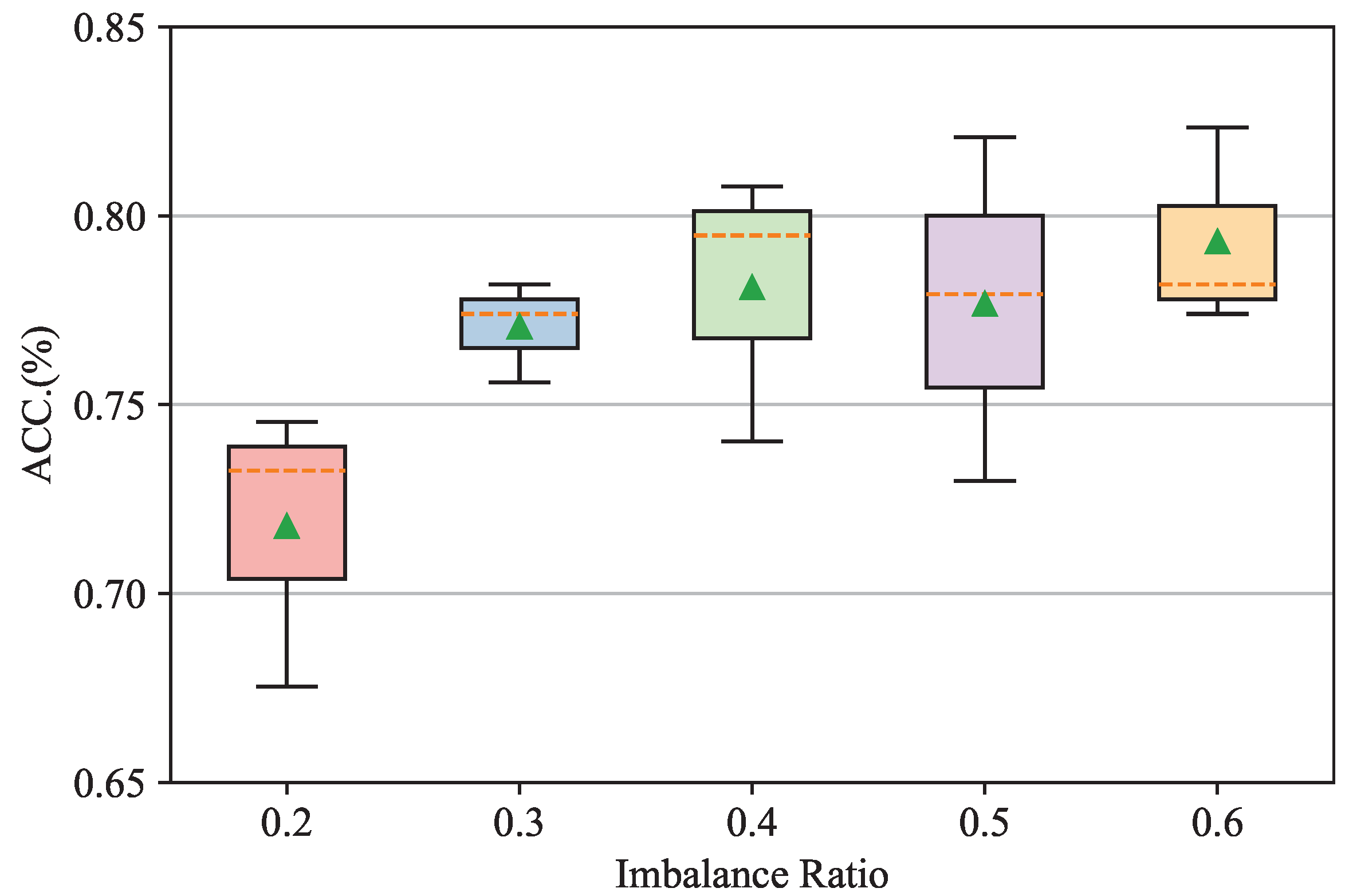
In this subsection, we analyze the performance of the proposed GATSMOTE based on different IRs to evaluate the algorithm’s robustness against different levels of the imbalance problem. The experiment is conducted in a well-constrained setting on Cora by varying the IRs at 0.2, 0.3, 0.4, 0.5, and 0.6 while holding all other settings constant. In accordance with the implementation (https://github.com/TianxiangZhao/GraphSmote (accessed on 20 May 2022)) of related work [12], the IR refers here to the ratio of the number of samples from the minority class to the number of samples from the majority class. The smaller the IR, the smaller the number of samples in the minority class. Experimental results are reported in Figure 2. The whiskers of boxplots are the range of accuracies over three-time experiments, and the line (green markers) inside the boxplots denotes the medium (mean) value of classification accuracies. Figure 2 displays that the performance of the proposed GATSMOTE improves as the IR increases. Such a phenomenon may have arisen because an increasing number of minority class samples can help the proposed method augment these samples and related edges to further debias the imbalanced node classification task and realize better performance. We also acknowledge that the standard variance remains at the same level as the IR rises. This pattern may be due to two reasons: the limited volume of the Cora dataset and the limited growth in sample size (i.e., the sample cannot adequately eliminate randomness during training).

4.2.3. Influence of Oversampling Scale

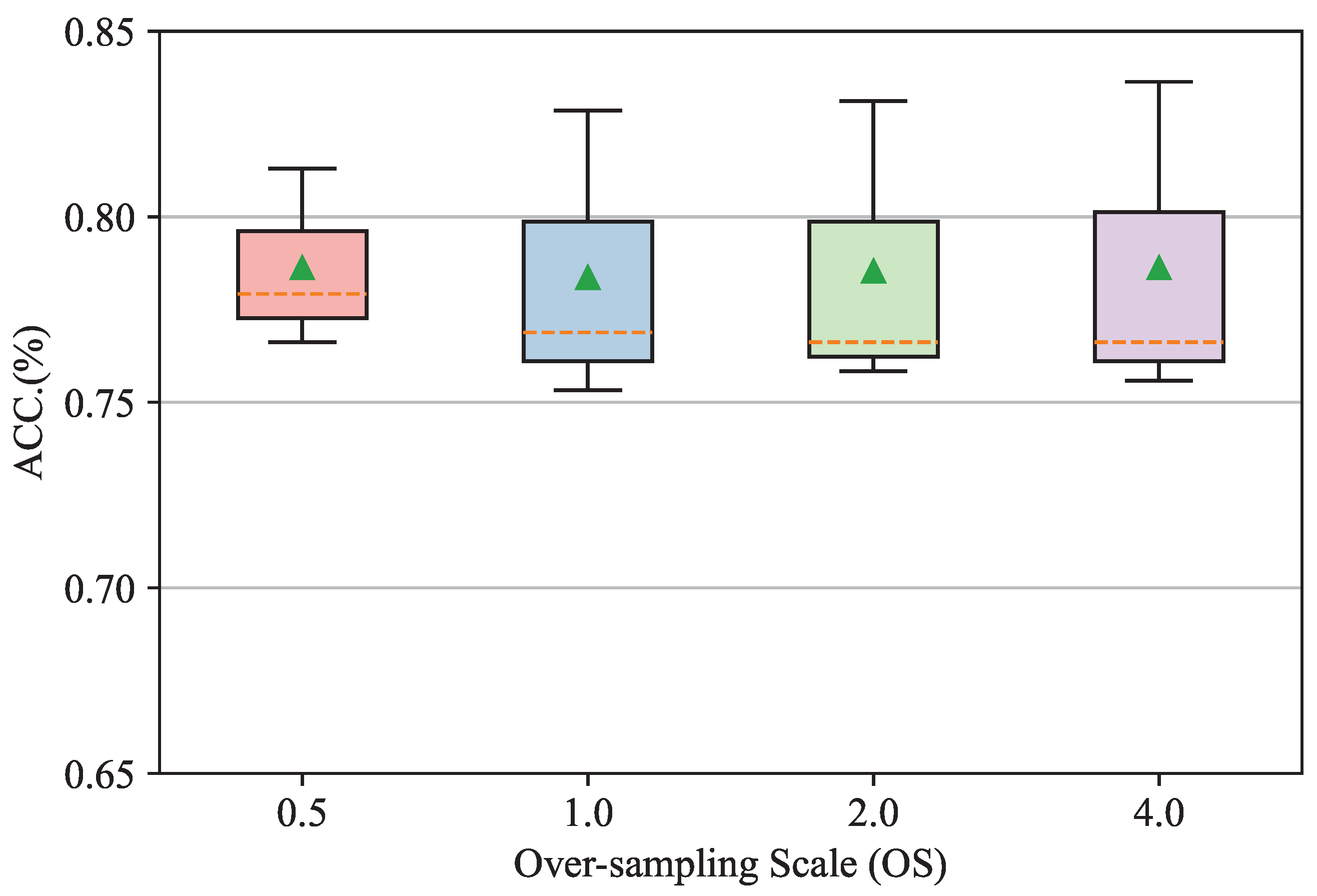
The oversampling scale determines the number of augmented minority class samples and thus is always considered a key factor affecting the performance of class-imbalanced node classification tasks. In this subsection, we conduct sensitivity experiments to evaluate the proposed method with different numbers of oversampling samples to explore the effects of oversampling scales. This experiment is conducted in a well-constrained setting on Cora by varying the oversampling scales at 0.5, 1.0, 2.0, and 4.0 under an IR of 0.5; all other settings are fixed. Per the implementation (https://github.com/TianxiangZhao/GraphSmote (accessed on 20 May 2022)) in related work [12], the oversampling scale refers here to the ratio of the number of augmented samples from the minority class to the number of original samples from the minority class. The smaller the IR, the smaller the number of augmented samples in the minority class. Experimental results are reported in Figure 2. The whiskers of boxplots are the range of accuracies over three-time experiments, and the line (green markers) inside the boxplots denotes the medium (mean) value of classification accuracies. Figure 3 illustrates that as the oversampling scales increase, the highest accuracies under the corresponding oversampling scale rise consistently, although the average accuracy expectancy does not show a significant difference. We assume that this phenomenon may have occurred given the limited number of minority class samples. Oversampling enamors augmented samples can help the model learn the patterns of minority classes and debiasing but raises the risk of overfitting on limited patterns of minority class samples. The overfitted models therefore have a residual effect on the average accuracy expectancy.

4.2.4. Influence of Attention Mechanism

Extensive studies have adopted deep graph structure learning [31] to infer the graph structure based on node representations in graphs. This subsection further explores well-adopted algorithms for deep structure learning and adapts them to our proposed GATSMOTE framework as an alternative to using the attention mechanism as an edge generator. In detail, we compare our proposed method with three potential edge generators while keeping other settings constant: (1) GATSMOTE w/Cosine Edge: We suggest using a linear layer to map node representations into the latent space and calculate the cosine distance between nodes in the latent space as corresponding edge weights. Mathematically, Equations (8), (9) and (13) can be replaced with $a_{vu}=\frac{{\left(\mathbf{W}{\mathbf{h}}_v\right)}^T\left(\mathbf{W}{\mathbf{h}}_u\right)}{∥\mathbf{W}{\mathbf{h}}_v∥∥\mathbf{W}{\mathbf{h}}_u∥}$. (2) GATSMOTE w/Gaussian Edge: We suggest using a linear layer to map node representations into the latent space and calculate the Gaussian kernel between nodes in the latent space as corresponding edge weights. Mathematically, Eqiations (8), (9) and (13) can be replaced with $a_{vu}=e^{-\frac{{∥\mathbf{W}{\mathbf{h}}_v-\mathbf{W}{\mathbf{h}}_u∥}^2}{\sigma }},\sigma =2$. (3) GATSMOTE w/Inner Edge: We suggest using a linear layer to map node representations into the latent space and calculate the inner product between nodes in the latent space as corresponding edge weights. This technique is effectively a GraphSMOTE variant. Mathematically, Equations (8), (9) and (13) can be replaced with $a_{vu}={\left(\mathbf{W}{\mathbf{h}}_v\right)}^T\left(\mathbf{W}{\mathbf{h}}_u\right)$. It is worth noting that to the best of our knowledge, no existing work has applied these strategies to class-imbalanced node classification tasks.

Table 3. Comparison experiments of edge construction operations based on the node-embedding space. This table illustrates the AUC-ROC of edge construction operations based on imbalance ratios.

Method	Cora
	$IR=0.2$	$IR=0.4$	$IR=0.6$
GATSMOTE w/Cosine Edge	$0.943$	$0.955$	$0.955$
GATSMOTE w/Gaussian Edge	$0.945$	$0.957$	$0.958$
GATSMOTE w/Inner Edge	$0.947$	$0.956$	0.960
GATSMOTE w/GATConv	0.950	0.957	0.958

The best results are highlighted in bold.

lists the comparison results of different edge construction operations for AUC-ROC metrics with respect to three IR levels. The proposed framework and designed loss functions appear to optimize all edge construction operations, and the overall performance achieves satisfactory accuracies of more than 0.94%. No matter which edge construction operation is applied, the performance of the proposed method improves as the IR increases. This trend likely manifests because a larger number of minority class samples can help the models learn to capture structural patterns between minority class samples to construct precise edges and debias the class imbalance. In particular, the proposed GATSMOTE w/GATConv achieves superior performance with most IRs. The performance gap is largest when the IR is low (i.e., in the extremely hard case where known minority class samples are highly limited). The experimental results demonstrate GATConv’s ability to learn complex structural patterns given limited samples with the help of the attention mechanism.

To explore the capacities of different edge construction operations in greater depth, we consider the hard case in edge construction: node representations exist in a high-dimensional space where a variety of distance (similarity) metrics will fail. We perform experiments in which a pre-trained feature extractor is not assessable and the raw representations of nodes serve as the GATSMOTE input (i.e., ${\tilde{\mathbf{H}}}^0=\mathbf{X}\cup SMOTE\left(\mathbf{X}\right)$ (Line 16 in Algorithm 1)). In this case, ${\tilde{\mathbf{H}}}^0$ refers to 1433-dimensional sparse raw representations on the Cora dataset instead of 256-dimensional dense feature representations extracted by a GATCov layer. We subsequently evaluate the proposed GATSMOTE with different edge construction operations under IRs in the range of 0.2, 0.3, 0.4, and 0.5. Each experiment is carried out three times with average accuracies reported in

Table 4. Sensitivity analysis of the parameters of loss components.

Metrics		${\mathit{\lambda }}_2$
		0	0.002	0.004	0.006	0.008	0.01
${\lambda }_1$	0	0.7195	0.7515	0.7368	0.7446	0.7749	0.7766
	0.02	0.7751	0.7513	0.7722	0.7799	0.7861	0.7829
	0.04	0.7828	0.7833	0.7815	0.7889	0.7890	0.7902
	0.06	0.7841	0.7886	0.7877	0.7850	0.7867	0.7842
	0.08	0.7842	0.7821	0.7860	0.7841	0.7823	0.7858
	0.1	0.7840	0.7814	0.7824	0.7823	0.7822	0.7850

The best results are highlighted in bold.

.

Table 5. Comparison experiments of edge construction operations based on raw node representations. This table illustrates the accuracies of edge construction operations based on imbalance ratios.

Method	Cora
	$IR=0.2$	$IR=0.3$	$IR=0.4$	$IR=0.5$
GATSMOTE w/Cosine Edge	$0.5325$	$0.6303$	$0.6866$	$0.7134$
GATSMOTE w/Gaussian Edge	$0.5706$	$0.6571$	$0.6970$	$0.7126$
GATSMOTE w/Inner Edge	$0.5792$	$0.6528$	$0.6926$	$0.7221$
GATSMOTE w/GATConv	0.5896	0.6710	0.7039	0.7307

The best results are highlighted in bold.

reveals that compared with Table 2, the performance of GATSMOTE-based models declines when the IR is set to 0.5. This phenomenon demonstrates that the pre-trained feature extractor is beneficial due to the effective dimension reduction of node representations, without which edge construction based on the original high-dimensional sparse feature representations would be meaningless and lead to suboptimal augmentation results. Additionally, the proposed GATSMOTE w/GATConv achieves the best performance irrespective of the IR. Especially when the IR is low (IR = 0.2), the proposed GATSMOTE w/GATConv outperforms GATSMOTE w/Cosine Edge at a large margin of 5%. GATConv can automatically learn the relationships between nodes based on the attention mechanism with better robustness than pre-defined distance/similarity measurements. In summary, the experimental results support the effectiveness of GATConv for edge estimation, even for high-dimensional raw representations.

4.2.5. Parameter Sensitivity Analysis

The most important hyperparameters in the proposed GATSMOTE include ${\lambda }_1$ and ${\lambda }_2$ in Equation (16). These hyperparameters weight the objective function of $L_{locality}$ and $L_{shortest}$ and demonstrate the importance of trade-off in the classification objective, Hypothesis 1, and Hypothesis 2. In this subsection, we conduct sensitivity experiments to evaluate the proposed method with different ${\lambda }_1$ and ${\lambda }_2$ in the range of 0, 0.02, 0.04, 0.06, 0.08, 0.1 and 0, 0.002, 0.004, 0.006, 0.008, 0.01, respectively, to explore the effects of weighting hyperparameters. The experiment is conducted in a well-constrained setting on Cora by fixing the IR at 0.5. Each experiment is performed three times with average accuracies reported in Table 4. When ${\lambda }_1$ is fixed at 0, the model accuracy increases as ${\lambda }_2$ increases. Compared with the accuracy of the model at ${\lambda }_2=0$, the accuracy of the model at ${\lambda }_2=0.01$ rises by about 6%. The same phenomenon occurs when ${\lambda }_2$ is fixed at 0 and ${\lambda }_1$ is changed. These phenomena illustrate that each loss function contributes to the optimization objective.

Meanwhile, when ${\lambda }_1$ and ${\lambda }_2$ change simultaneously, the final accuracy does not improve with a simultaneous increase in ${\lambda }_1$ and ${\lambda }_2$. For example, when ${\lambda }_2$ is 0.01, raising ${\lambda }_1$ causes the model performance to increase and then decrease. The optimization directions of the two assumptions are therefore not completely consistent, and a trade-off exists for ${\lambda }_1$ and ${\lambda }_2$ in class-imbalanced node classification tasks. We thus recommend weighting ${\lambda }_1$ and ${\lambda }_2$ on the same scale and then adjusting ${\lambda }_1$ to achieve better results. In this case, we suggest ${\lambda }_1=0.04$, ${\lambda }_2=0.01$.

4.3. Ablation Study

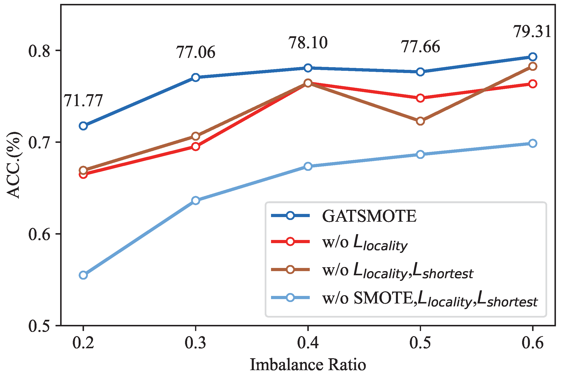
In this subsection, we conduct ablation studies on the Cora dataset to evaluate the performance gain of different designs. We specifically compare our proposed GATSMOTE with three ablated versions: (1) GATSMOTE w/o $L_{locality}$: To demonstrate the performance gain of $L_{locality}$, we first remove the term $L_{locality}$ from Equation (16) and name the ablated model trained without $L_{locality}$ as GATSMOTE w/o $L_{locality}$. (2) GATSMOTE w/o $L_{locality}$,$L_{shortest}$: Consistent with $L_{locality}$, we further ablate the term of $L_{shortest}$ and name the ablated model trained with only $L_{node}$ as GATSMOTE w/o $L_{locality}$,$L_{shortest}$. (3) GATSMOTE w/o SMOTE: To evaluate the performance gain attributable to the node augmentation and edge generator, we further remove the node augmentation operations and edge constructor operations to obtain the performance of vanilla GAT with consistent parameter numbers from the proposed methods. The experiment is conducted in a well-constrained setting on Cora by fixing the IR at 0.5. Each experiment is performed three times with average accuracies reported in Figure 4.

The curve of GATSMOTE almost completely encloses the curves of GATSMOTE w/o $L_{locality}$, w/o $L_{locality}$,$L_{shortest}$, and w/o SMOTE, demonstrating that the proposed versions of GATSMOTE are superior to all ablated versions of the proposed GATSMOTE. In other words, all design modules contribute to the overall performance, without which the performance would decline. Additionally, a performance gap occurs between GATSMOTE and GATSMOTE w/o $L_{locality}$,$L_{shortest}$ regardless of IR. This phenomenon demonstrates that Hypotheses 1 and 2 work with different IRs. Finally, the proposed GATSMOTE outperforms GATSMOTE w/o SMOTE by a large margin, indicating that the attention mechanism itself (without a special design) is inadequate for debiasing in class-imbalanced node classification tasks. The proposed design in which the attention mechanism is adopted for node augmentation and edge construction is essential.

4.4. Toy Experiments on Real EEG Data

In this subsection, we conduct our oversampling algorithm on the real EEG data: Bonn dataset [32]. It has five distinct subsets, which are denoted by Z, O, N, F, and S. Each subset has 100 single-channel segments. Each segment has a 23.6 s duration with 4097 samples. Sets Z and O are the surface EEG signals from five healthy peple while they are with eyes open and eyes closed. Sets N and F are the intracranial EEG signals from five epilepsy patients during seizure-free intervals. Set S also contains the intracranial EEG signals from five epilepsy patients; however, the signals are collected during the seizure.

Our analysis divides and shuffles 4097 samples within each segment into 23 batches. Each batch contains 178 samples. We sample 5 batches from 23 batches and 5 segments from 100 segments. Now, we have 5 batches × 5 classes × 5 segments = 125 pieces of EEG signals. Each EEG signal piece is 178-dimensional. We aim to detect the ictal EEG signals from normal EEG signals. Therefore, it is a binary classification problem (ZONF vs. S) with the class imbalance. As the recordings in this dataset are from single-channel, we reconstruct the edges between them based on their Pearson correlation followed by a manually set threshold [11]. Until now, we have converted the raw Bonn dataset into a graph data $\mathbf{G}=\{\mathbf{V},\mathbf{A},\mathbf{X}\}$, where $\mathbf{V}$ is a set of 125 nodes; $\mathbf{A}\in {\mathbb{R}}^{125\times 125}$ is the adjacency matrix; and $\mathbf{X}\in {\mathbb{R}}^{125\times 178}$ is the feature matrix. $\mathbf{Y}\in {\mathbb{R}}^{125\times 2}$ denote the label information, with the imbalance ratio at 0.25. It is worth noting that the dimension of the EEG signal, 178, is lower than the dimension of the graph benchmark Cora. Therefore, we use a lower hidden layer dimension of 32 in the networks, and the attention head number is reduced to 2. The test results are reported in

Table 6. Comparison of approaches for imbalanced node classification on Bonn dataset.

Method	CoraBonn
	ACC	AUC-ROC	F-Score
Origin	0.7895	0.5167	0.4412
Oversample	0.7895	0.7167	0.4412
SMOTE	0.7895	0.6000	0.4412
GraphSMOTE	0.7895	0.6500	0.7286
GATSMOTE	0.8947	0.7833	0.8417

The best results are highlighted in bold.

.

From Table 6, we can find that the classification results without dealing with the data imbalance problem are biased toward the majority category, achieving low AUC-ROC. When using the traditional techniques, such as oversampling and SMOTE [8], the AUC of the classifier has improved, which means that the classifier can distinguish positive and negative samples against imbalance problems underparts of thresholds. However, the ACC and F-scores have not changed, indicating that the classifier is still biased. After applying GraphSMOTE, it can be found that the F-score of the classifier is further improved, indicating that techniques considering graph structure have a positive effect on recall. In the end, our GATSMOTE [12] achieved the best results on both accuracy, AUC, and F-score, which means that the model proposed in this paper inferring graph structure with attention mechanism can also effectively solve the imbalance problem for EEG datasets.

5. Discussion

Non-invasive neuro-imaging has proven to be an invaluable research tool for determining how the brain works. Using an electroencephalogram (EEG), with its portability and excellent temporal resolution, neuroscientists can image the brain’s psychological states in real time. However, EEG recordings are usually confounded by aberrant signals. These aberrant signals may arise from disconnected/broken electrodes. In addition to a “bad channel” during EEG recordings, eye movements and blink artifacts may also result in the aberrant signals that have several times higher magnitude than the normal ones [33]. Our GATSMOTE is proposed to not ignore the nodes from the minority classes and improve the node classification performance. It can be usefully applied to other engineering disciplines with the class imbalance problem, especially for detecting aberrant EEG signals in various scenarios.

• Denoising EEG signals has become an important research topic in signal processing. As mentioned earlier, EEG signals are heavily corrupted with artifacts and broken electrodes. These noises would restrict the applicability and reliability of brain–computer interfaces (BCI) [34]. In essence, detecting noises is a class imbalance problem, as the number of noises is fewer than normal. Applying our proposed GATSMOTE in denoising EEG signals, the disconnected/broken electrodes can be naturally regarded as the nodes from the minority class. The interpolation method utilized in our algorithm can generate synthetic signals for the broken electrodes. Our proposed edge generator can not only help the disconnected electrodes connect to the brain network but also can add new connections for information passing at a low cost.
• EEG-based attention examination enables the real-time and continuous examination of subjects’ mental states and brain activities [35]. CPT and T. O. V. A. tests are two traditional attention measuring methods applied to measure the attention of subjects when they receive a visual or auditory stimulus during a particular test [35]. However, they cannot measure and process the brain signals in real time like an EEG device. Applying our algorithm in EEG-based examination, the signals of low or anomalously high attention levels can be detected more accurately. We can treat the signals measuring abnormal attention levels as the nodes from minority classes. Our algorithm would generate synthetic nodes and connect them to the original graph via our edge generator. Better detection of abnormal attention levels would help inform teachers when their students decrease attention. Furthermore, it would increase the efficiency of teaching.
• Eye tracker systems record the position and movement of eyes in relation to the head [36]. Aberrant signals induced from eye movements are usually considered as artifacts that need to be removed during pre-processing. However, these artifacts are also a valuable source of data in BCI, which is useful for delivering information and then implementing the functions of mouses or keyboards [37]. Therefore, detecting the signals induced by eye movements would further help the communication with computers. Our proposed algorithm can be applied to achieve this goal, as the synthetic signals of eye movements would be oversampled. Moreover, the relationships between different channels of EEG would also be preserved and even enhanced via our edge generator.

6. Conclusions and Future Work

The class imbalance problem is widespread in real-world application scenarios, and many oversampling methods have been suggested to alleviate this concern. However, existing solutions are still limited to graph data with the class imbalance problem. One of the greatest challenges is that available oversampling methods cannot directly connect synthetic nodes to the original graph. Even so, the class imbalance problem remains undervalued in brain science. This issue persists in many brain science applications, such as “bad-channel” detection [1] and artifact detection [2]. In this paper, while addressing the small network architecture of the brain network, we propose a novel edge generator to add relation information between synthetic nodes and the original graph. Experiments on the benchmark dataset, Cora, demonstrate the superiority of our proposed model: it outperforms all other baselines. We conduct ablation studies to clarify the effects of our proposed regularization on node classification. Parameter sensitivity analysis is also carried out to determine the sensitivity of our two proposed regularizations. Results show that each of the two hypotheses contributes to node classification.

Although this work demonstrates the effectiveness of imbalanced node classification on the benchmark, several directions still need further investigation. First, the experimental verification of real EEG data is still limited. In this work, we conduct our proposed GATSMOTE on the sampled Bonn dataset [32], which records the single-channel brain activity of the healthy people and epilepsy patients. However, more experiments on real EEG data are still needed, such as EEG measurements from different brain regions and channels. Second, in this work, we mainly verify the outperformance of GATSMOTE in classifying nodes from the minority classes. The effectiveness of our proposed GATSMOTE on the broken/disconnected is still not verified explicitly. We aim to study the performance of our algorithm by varying the number of lost nodes in our subsequent work. Third, we would like to extend our oversampling algorithm to more application scenarios, such as extending our GATSMOTE to the eye tracker system to generate more useful signals similar to the artifacts induced by eye movements.

References

- Tuyisenge, V.; Trebaul, L.; Bhattacharjee, M.; Chanteloup-Forêt, B.; Saubat-Guigui, C.; Mîndruţă, I.; Rheims, S.; Maillard, L.; Kahane, P.; Taussig, D.; et al. Automatic bad channel detection in intracranial electroencephalographic recordings using ensemble machine learning. Clin. Neurophysiol. 2018, 129, 548–554. [Google Scholar] [CrossRef] [PubMed]
- Echtioui, A.; Zouch, W.; Ghorbel, M.; Slima, M.B.; Hamida, A.B.; Mhiri, C. Automated EEG Artifact Detection Using Independent Component Analysis. In Proceedings of the 2020 5th International Conference on Advanced Technologies for Signal and Image Processing (ATSIP), Sousse, Tunisia, 2–5 September 2020; pp. 1–5. [Google Scholar]
- Li, A.; Huynh, C.; Fitzgerald, Z.; Cajigas, I.; Brusko, D.; Jagid, J.; Claudio, A.O.; Kanner, A.M.; Hopp, J.; Chen, S.; et al. Neural fragility as an EEG marker of the seizure onset zone. Nat. Neurosci. 2021, 24, 1465–1474. [Google Scholar] [CrossRef] [PubMed]
- Singh, A.; Jain, A. Adaptive credit card fraud detection techniques based on feature selection method. In Advances in Computer Communication and Computational Sciences; Springer: Singapore, 2019; pp. 167–178. [Google Scholar]
- Song, H.M.; Woo, J.; Kim, H.K. In-vehicle network intrusion detection using deep convolutional neural network. Veh. Commun. 2020, 21, 100198. [Google Scholar] [CrossRef]
- Spelmen, V.S.; Porkodi, R. A review on handling imbalanced data. In Proceedings of the 2018 International Conference on Current Trends towards Converging Technologies (ICCTCT), Coimbatore, India, 1–3 March 2018; pp. 1–11. [Google Scholar]
- Ali, H.; Salleh, M.N.M.; Saedudin, R.; Hussain, K.; Mushtaq, M.F. Imbalance class problems in data mining: A review. Indones. J. Electr. Eng. Comput. Sci. 2019, 14, 1560–1571. [Google Scholar] [CrossRef]
- Chawla, N.V.; Bowyer, K.W.; Hall, L.O.; Kegelmeyer, W.P. SMOTE: Synthetic minority over-sampling technique. J. Artif. Intell. Res. 2002, 16, 321–357. [Google Scholar] [CrossRef]
- Joudaki, A.; Salehi, N.; Jalili, M.; Knyazeva, M.G. EEG-based functional brain networks: Does the network size matter? PLoS ONE 2012, 7, e35673. [Google Scholar] [CrossRef] [PubMed] [Green Version]
- Zhao, Y.; Dong, C.; Zhang, G.; Wang, Y.; Chen, X.; Jia, W.; Yuan, Q.; Xu, F.; Zheng, Y. EEG-Based Seizure detection using linear graph convolution network with focal loss. Comput. Methods Programs Biomed. 2021, 208, 106277. [Google Scholar] [CrossRef]
- Tzimourta, K.D.; Astrakas, L.G.; Tsipouras, M.G.; Giannakeas, N.; Tzallas, A.T.; Konitsiotis, S. Wavelet based classification of epileptic seizures in EEG signals. In Proceedings of the 2017 IEEE 30th International Symposium on Computer-Based Medical Systems (CBMS), Thessaloniki, Greece, 22–24 June 2017; pp. 35–39. [Google Scholar]
- Zhao, T.; Zhang, X.; Wang, S. Graphsmote: Imbalanced node classification on graphs with graph neural networks. In Proceedings of the 14th ACM International Conference on Web Search and Data Mining, Virtual Event, Israel, 8–12 March 2021; pp. 833–841. [Google Scholar]
- Liao, X.; Vasilakos, A.V.; He, Y. Small-world human brain networks: Perspectives and challenges. Neurosci. Biobehav. Rev. 2017, 77, 286–300. [Google Scholar] [CrossRef]
- Achard, S.; Bullmore, E. Efficiency and cost of economical brain functional networks. PLoS Comput. Biol. 2007, 3, e17. [Google Scholar] [CrossRef]
- Ma, Y.; Liu, X.; Shah, N.; Tang, J. Is Homophily a Necessity for Graph Neural Networks? arXiv 2021, arXiv:2106.06134. [Google Scholar]
- Cao, P.; Zhao, D.; Zaiane, O. An optimized cost-sensitive SVM for imbalanced data learning. In Pacific-Asia Conference on Knowledge Discovery and Data Mining; Springer: Berlin/Heidelberg, Germany, 2013; pp. 280–292. [Google Scholar]
- Wu, G.; Chang, E.Y. Class-boundary alignment for imbalanced dataset learning. In Proceedings of the ICML 2003 Workshop on Learning from Imbalanced Data Sets II, Washington, DC, USA, 21–24 August 2003; pp. 49–56. [Google Scholar]
- Sahare, M.; Gupta, H. A review of multi-class classification for imbalanced data. Int. J. Adv. Comput. Res. 2012, 2, 160. [Google Scholar]
- Sun, Y.; Wong, A.K.; Kamel, M.S. Classification of imbalanced data: A review. Int. J. Pattern Recognit. Artif. Intell. 2009, 23, 687–719. [Google Scholar] [CrossRef]
- Haixiang, G.; Yijing, L.; Shang, J.; Mingyun, G.; Yuanyue, H.; Bing, G. Learning from class-imbalanced data: Review of methods and applications. Expert Syst. Appl. 2017, 73, 220–239. [Google Scholar] [CrossRef]
- Wu, Z.; Pan, S.; Chen, F.; Long, G.; Zhang, C.; Philip, S.Y. A comprehensive survey on graph neural networks. IEEE Trans. Neural Netw. Learn. Syst. 2020, 32, 4–24. [Google Scholar] [CrossRef] [PubMed] [Green Version]
- Hamilton, W.; Ying, Z.; Leskovec, J. Inductive representation learning on large graphs. Adv. Neural Inf. Process. Syst. 2017, arXiv:1706.02216. [Google Scholar]
- Veličković, P.; Cucurull, G.; Casanova, A.; Romero, A.; Lio, P.; Bengio, Y. Graph attention networks. arXiv 2017, arXiv:1710.10903. [Google Scholar]
- Sen, P.; Namata, G.; Bilgic, M.; Getoor, L.; Galligher, B.; Eliassi-Rad, T. Collective classification in network data. AI Mag. 2008, 29, 93. [Google Scholar] [CrossRef] [Green Version]
- Wu, L.; Lin, H.; Gao, Z.; Tan, C.; Li, S. GraphMixup: Improving Class-Imbalanced Node Classification on Graphs by Self-supervised Context Prediction. arXiv 2021, arXiv:2106.11133. [Google Scholar]
- Yuan, B.; Ma, X. Sampling+ reweighting: Boosting the performance of AdaBoost on imbalanced datasets. In Proceedings of the 2012 International Joint Conference on Neural Networks (IJCNN), Brisbane, Australia, 10–15 June 2012; IEEE: Piscataway, NJ, USA, 2012; pp. 1–6. [Google Scholar]
- Ando, S.; Huang, C.Y. Deep over-sampling framework for classifying imbalanced data. In Proceedings of the Joint European Conference on Machine Learning and Knowledge Discovery in Databases, Skopje, Macedonia, 18-22 September 2017; pp. 770–785. [Google Scholar]
- Johnson, J.M.; Khoshgoftaar, T.M. Survey on deep learning with class imbalance. J. Big Data 2019, 6, 1–54. [Google Scholar] [CrossRef]
- Rout, N.; Mishra, D.; Mallick, M.K. Handling imbalanced data: A survey. In International Proceedings on Advances in Soft Computing, Intelligent Systems and Applications; Springer: Singapore, 2018; pp. 431–443. [Google Scholar]
- Bradley, A.P. The use of the area under the ROC curve in the evaluation of machine learning algorithms. Pattern Recognit. 1997, 30, 1145–1159. [Google Scholar] [CrossRef] [Green Version]
- Zhu, Y.; Xu, W.; Zhang, J.; Liu, Q.; Wu, S.; Wang, L. Deep graph structure learning for robust representations: A survey. arXiv 2021, arXiv:2103.03036. [Google Scholar]
- Andrzejak, R.G.; Lehnertz, K.; Mormann, F.; Rieke, C.; David, P.; Elger, C.E. Indications of nonlinear deterministic and finite-dimensional structures in time series of brain electrical activity: Dependence on recording region and brain state. Phys. Rev. E 2001, 64, 061907. [Google Scholar] [CrossRef] [PubMed] [Green Version]
- Mannan, M.M.N.; Kim, S.; Jeong, M.Y.; Kamran, M.A. Hybrid EEG—Eye tracker: Automatic identification and removal of eye movement and blink artifacts from electroencephalographic signal. Sensors 2016, 16, 241. [Google Scholar] [CrossRef] [PubMed] [Green Version]
- Brophy, E.; Redmond, P.; Fleury, A.; De Vos, M.; Boylan, G.; Ward, T.E. Denoising EEG signals for Real-World BCI Applications using GANs. Front. Neuroergonomics 2022, 2, 805573. [Google Scholar] [CrossRef]
- Katona, J. Examination and comparison of the EEG based Attention Test with CPT and TOVA. In Proceedings of the 2014 IEEE 15th International Symposium on Computational Intelligence and Informatics (CINTI), Budapest, Hungary, 19–21 November 2014; IEEE: Piscataway, NJ, USA, 2014; pp. 117–120. [Google Scholar]
- Katona, J. Analyse the Readability of LINQ Code using an Eye-Tracking-based Evaluation. Acta Polytech. Hung 2021, 18, 193–215. [Google Scholar] [CrossRef]
- Katona, J. A review of human–computer interaction and virtual reality research fields in cognitive InfoCommunications. Appl. Sci. 2021, 11, 2646. [Google Scholar] [CrossRef]
Figure 1.
Illustration of our proposed edge generator in GATSMOTE.
Figure 2.
Accuracies of proposed GATSMOTE for imbalanced node classification under different imbalance ratios.
Figure 3.
Accuracies of proposed GATSMOTE for imbalanced node classification under different upsampling scales for an imbalance ratio of 0.5.
Figure 4.
Accuracies ACC (%) of ablated versions of the proposed GATSMOTE for imbalanced node classification under different imbalance ratios.