An Active Learning Algorithm Based on the Distribution Principle of Bhattacharyya Distance

Abstract

Active learning is a method that can actively select examples with much information from a large number of unlabeled samples to query labeled by experts, so as to obtain a high-precision classifier with a small number of samples. Most of the current research uses the basic principles to optimize the classifier at each iteration, but the batch query with the largest amount of information in each round does not represent the overall distribution of the sample, that is, it may fall into partial optimization and ignore the whole, which will may affect or reduce its accuracy. In order to solve this problem, a special distance measurement method—Bhattacharyya Distance—is used in this paper. By using this distance and designing a new set of query decision logic, we can improve the accuracy of the model. Our method embodies the query of the samples with the most representative distribution and the largest amount of information to realize the classification task based on a small number of samples. We perform theoretical proofs and experimental analysis. Finally, we use different data sets and compare them with other classification algorithms to evaluate the performance and efficiency of our algorithm.

1. Introduction

With the significant improvement of computer science technology, machine learning has been highly valued in recent years. After solving functional problems, centered on machine learning, many fields have been developed quickly, such as support vector machines, deep learning, reinforce learning, etc. Synchronously with the performance improvement is the quantity and quality of the data set. For machine learning, the higher the accuracy, the more unlabeled data need to be labeled. Based on the current scale of machine learning, training a good model requires tens of thousands of labeled samples. The huge training cost has become an obstacle to putting machine learning into practical applications. Active learning, which greatly reduces the cost of training and learning by introducing artificial auxiliary markers in training, is undoubtedly one of the best solutions to the current training cost problem.

Research on active learning is mainly divided into three scenarios, member query synthesis, stream-based sample selection, and pool-based sample selection [1]. The active learning referred to in this paper is mainly based on pool scenarios [2], using a small number of labeled samples to infer the most useful samples in the overall sample and querying experts, so as to achieve low-cost labeled data to obtain high-precision trainers. Compared with traditional machine learning, its advantages are lower cost and higher accuracy. The training of the classifier is completed by selectively selecting high-quality samples.

However, the shortcoming of active learning as a solution to the cost problem is the training over-fitting caused by the sparse sample number and strong sample characteristics and differences in the optimization process. For this question, there are many answers given, such as the Query by Committee (QBC) [3], the largest average difference batch query, combined with self-paced learning, etc., all to solve the problem of only focusing on uncertainty but not the overall distribution of the sample in the active learning process. Among them, a reference [4] proposes to add the distance between distributions to the active learning algorithm so as to realize the scheme of extracting representative samples. This paper proposes an active learning algorithm based on Bhattacharyya distance as a method of measuring distributed distance, and proves the feasibility and superiority of this theory through theories analysis and experiments.

Contributions: The main contributions of our proposed active learning method are listed as follows:

1.

The kernel function is used to simulate the Bhattacharyya distance as a distribution distance measure for active learning. This method can express the degree of coincidence between distributions. By analyzing the Bhattacharyya distance between the unlabeled sample set and the labeled sample set, the imbalance of uncertainty and representativeness is removed.

2.

A new sample selection model is built to select more suitable samples from a large number of unlabeled samples for training.

3.

Through various experiments with different datasets, we have verified the superiority of the Bhattacharyya distance active learning compared with most traditional active learning algorithms.

2. Related Works

2.1. Active Learning

According to the traditional theory, the selective inquiry of samples from experts requires a specific selection criterion, deciding which parameters to choose as a reference. Uncertainty is usually used as the criterion for selecting samples, the original query framework based on uncertainty was proposed by Lewis and Gale in 1994 [5], and the higher the uncertainty, the more information the sample covers and the greater the contribution to the model. In different selection strategies, the method of measuring uncertainty is different. QBC, raised by Ray Liere in 1997, the sample that the committee disagrees with the most is the sample with the highest uncertainty; in a support vector machine-based algorithm, the uncertainty is determined by the distance between the sample and the boundary. In addition, there is Fisher information [6], probability confidence [7], information entropy [8], etc. which can be used as reference standards. In recent years, active learning has increasingly become an important research content in the field of machine learning and deep learning. Active deep learning has gradually become a new trend, such as combining a Bayesian network to use active learning to obtain uncertain information [9], and combining data reinforcement learning constitutes a Bayesian generative active learning method [10], or applies active learning to semantic segmentation, utilizes a committee query mechanism for information volume and representativeness criteria, and combines edge information clues to optimize semantic segmentation algorithms [11].

However, only using uncertainty as a standard will face an unavoidable problem, although uncertainty only screens samples that greatly improve the model; it does not take the diversity and distribution of the overall sample into account. With the small number of labeled samples, bias and overfitting occur.

Another criterion for selecting samples, representativeness [12], is proposed as a different way of thinking. The representativeness of a sample indicates how well it can represent other unlabeled samples. Through the overall distribution of the data, the distribution of a large number of unlabeled samples can be represented by a small number of samples. The idea of clustering is usually referenced, and the use of clustering structure to select samples is also a common method. In this case, compared to the uncertainty standard, only high-efficiency data are selected. Sample combinations from different groups or different categories are the objects selected by the representative standard, but this method largely depends on the quality of data clustering. Similarly, there is diversity, systemicity, and principle.

There are many existing learning methods that try to combine these standards, such as active learning based on self-paced learning newly raised in 2019 named Self-paced Active Learning (SPAL) [13], active learning based on graph diversity, and representative batch mode active learning. The main idea is to introduce representativeness or diversity while pursuing the uncertainty of query samples. The basic idea of this paper is also to use the distribution distance to express the representativeness and diversity of the sample. Previously, the maximum average difference was used. KL divergence [14], JS divergence [15], etc. were used as the measurement of the distribution distance [16]. In this paper, the Bhattacharyya distance will be used as the measurement like representative active learning.

2.2. Bhattacharyya Distance

In statistics, the Bhattacharyya distance is used to measure the similarity between two discrete or continuous probability distributions [17]. It is closely related to the Bhattacharyya coefficient, which measures the amount of overlap between two statistical samples. At the same time, the Bhattacharyya coefficient can be used to determine whether two samples are considered to be relatively close, and it can be used to measure the separability of the two classes.

For the probability distributions M and N defined in the same domain [18], the Bhattacharyya distance is defined as:

$$D_B\left(M,N\right)=-ln\left(BC\left(M,N\right)\right)$$

(1)

where $BC\left(M,N\right)$ is the Bhattacharyya coefficient of probability distributions M and N. For discrete probability distributions, the Bhattacharyya coefficients of M and N are defined as:

$$BC\left(M,N\right)=\sum _{x\in X}\sqrt{M\left(x\right)N\left(x\right)}$$

(2)

For continuous probability distributions, the Bhattacharyya coefficients of M and N are defined as:

$$BC\left(M,N\right)={\int }_X\sqrt{M\left(x\right)N\left(x\right)}dx$$

(3)

For two probability distributions, the larger the Bhattacharyya coefficient and the closer the Bhattacharyya distance to zero, the more similar are the two probability distributions. Conversely, the closer the Bhattacharyya distance is to zero, the more the Bhattacharyya distance is approaching infinity, and the more dissimilar the two probability distributions are. The value of the Bhattacharyya coefficient between the two probability distributions will increase with the increase of the same part of the two target samples. In theory, if the two samples have no overlap at all or almost no overlap, the Bhattacharyya coefficient will be equal to zero or approaching zero, the Bhattacharyya distance will approach infinity. At this time, we can consider that the correlation between the two probability distributions is very low.

In literature [19], the Bhattacharyya distance is extended as an application of a quantitative uncertainty measure, and a likelihood function based on the concept of distance is established. The innovation of this paper is expressing Bhattacharyya distance as the degree of approximation between distributions to measure its representativeness, which has never been tried in sample selection instead of feature selection. Therefore, we introduce Bhattacharyya distance as a metric of distribution distance into active learning to balance uncertainty and representativeness, and combine the two to realize accurate queries of unlabeled samples.

2.3. Kernel Methods

The support vector machine maps the input space to the high-dimensional space through a certain nonlinear variable $\varphi \left(x\right)$. If the solution of the support vector machine only uses the inner product operation, and there is a certain function $K\left(x,x^{\prime }\right)$, which is exactly equal to the inner product in the high-dimensional space, that is, $K\left(x,x^{\prime }\right)\le 〈\varphi \left(x\right)·\varphi \left(x^{\prime }\right)〉$. Then, the support vector machine does not need to calculate the complex nonlinear transformation, and the inner product of the nonlinear transformation is directly obtained from this function $K\left(x,x^{\prime }\right)$, which greatly simplifies the calculation. Such a function $K\left(x,x^{\prime }\right)$ is called a kernel function. In addition, the kernel function in the experiment is $K\left(x_i,x_j\right)=\varphi {\left(x_i\right)}^T\varphi \left(x_j\right)$, where $\varphi \left(x_i\right)$ and $\varphi \left(x_j\right)$ are the nonlinear mapping characteristic functions of two distribution on Reproducing Kernel Hilbert Space (RKHS), respectively. As early as 1964, Aizermann et al. introduced this technology to the field of machine learning in the study of potential function methods, but it was not until 1992 that Vapnik et al. used this technology to successfully extend linear SVMs to nonlinear SVMs, and its potential was not fully tapped.

3. Upper Bound of Active Learning Based on Bhattcharyya Distance

In this work, we mainly give the feasibility of our method under the binary classification problem. Suppose we have a data set $S=\left\{x_1,x_2,\cdots ,x_n\right\}$, which has d dimensions. First, we first provide l labeled data. We will write it as $L=\left\{\left(x_1,y_1\right),\left(x_2,y_2\right),\cdots ,\left(x_l,y_l\right)\right\}$, where y is the label of $\left\{-1,1\right\}$ denoted as sample x. Except for l labeled data, all the other labels are unlabeled labels, and $u=n-l$ is the number of unlabeled labels, and U is the unlabeled data set, so we record $U=\left\{x_{l+1},x_{l+2},\cdots ,x_n\right\}$. The method of active learning is to obtain b optimal sample sets Q from the unlabeled data set U through a designed decision-making method, query their labels and place them in the labeled sample set L. The purpose is to learn a suitable classifier from the input samples and training distribution to minimize the following expected risks:

$$E_D\left(l\left(z\right)\right)={\int }_{Z}l\left(z\right)P\left(x|y\right)p\left(y\right)dz$$

(4)

According to Rademacher complexity and McDiarmid’s inequality [20], the expected risk can be expressed as:

$$E_D\left(l\left(z\right)\right)\le {\widehat{E}}_S\left(l\left(z\right)\right)+2R_n\left(L\right)+\sqrt{\frac{ln1/\delta }{n}}$$

(5)

where ${\widehat{E}}_S\left(l\left(z\right)\right)=\frac{1}{\left|S\right|}{\displaystyle \sum _{z\in S}}l\left(z\right)$ is the empirical average of empirical risk, and $R_n\left(L\right)$ is the Rademacher complexity. According to the reference [13], the premise of Empirical risk minimization (ERM) is that the empirical risk and the expected risk are the same distribution, but it is not necessarily true in active learning. In order to extend the principle of empirical risk minimization to active learning, assuming that the labeled data are obtained from the q distribution, the original distribution is an equal q distribution, and the inequality can be rephrased as:

$$E_D\left(l\left(z\right)\right)\le \left(E_D\left(l\left(z\right)\right)-E_Q\left(l\left(z\right)\right)\right)+{\widehat{E}}_Q\left(l\left(z\right)\right)+const$$

(6)

The difference between the expected error of the query distribution and the overall distribution can be rewritten as:

$$\underset{\widehat{g}\in C\left(x\right)}{sup}{\int }_x\widehat{g}\left(x\right)p\left(x\right)dx-{\int }_x\widehat{g}\left(x\right)q\left(x\right)dx$$

(7)

Supposing that $p\left(x,y\right)=p\left(x\right)p\left(y|x\right)$, $q\left(x,y\right)=q\left(x\right)q\left(y|x\right)$ and $g\left(x\right)={\int }_{y}l\left(f\left(x\right),y\right)p\left(y|x\right)dy$, where g is bounded and measurable, we suppose there is a continuous function $\widehat{g}$ such that the formula above is satisfied. According to the definition of Bhattacharyya distance, we have:

$$\begin{array}{cc}\hfill BD[C,p(x),q(x\left)\right]& =-ln\left({\int }_x\sqrt{p\left(x\right)q\left(x\right)}dx\right)\hfill \\ \hfill & =ln\frac{1}{{\int }_x\sqrt{p\left(x\right)q\left(x\right)}dx}\hfill \end{array}$$

(8)

Therefore, according to Refs. [21,22], the Bhattacharyya distance can be expressed in the following two forms, and from the definition in RKHS, the Bhattacharyya distance can also be expressed as the third form:

$$\begin{array}{cc}\hfill JB& =\frac{1}{4}ln\left(\frac{1}{4}\left(\frac{\sigma {}_p^2}{\sigma {}_q^2}+\frac{\sigma {}_q^2}{\sigma {}_p^2}+2\right)\right)+\frac{1}{4}\left(\frac{{\left({\mu }_p-{\mu }_q\right)}^2}{\sigma {}_p^2+\sigma {}_q^2}\right)\hfill \\ \hfill JB& ={\xi }_{11}+{\xi }_{22}-{\xi }_{12},{\xi }_{ij}=s_i^T{K}_{ij}{s}_j+s_i^T\left(\begin{array}{cc}{K}_{i1}& K_{i2}\end{array}\right)B\left(\begin{array}{c}{K}_{1j}\\ K_{2j}\end{array}\right)s_j\hfill \\ \hfill JB& =ln\frac{1}{{\sum }_{x_i\in L\cup U}^{x_j\in L\cup Q}\sqrt{K\left(x_i,x_j\right)}}\hfill \end{array}$$

(9)

The denominator can be expressed as:

$$\begin{array}{cc}\hfill & {\int }_x\widehat{g}\left(x\right)p\left(x\right)dx-{\int }_x\widehat{g}\left(x\right)q\left(x\right)dx\hfill \\ \hfill & =\frac{{\left({\int }_x\widehat{g}\left(x\right)p\left(x\right)dx\right)}^2-{\left({\int }_x\widehat{g}\left(x\right)q\left(x\right)dx\right)}^2}{{\int }_x\widehat{g}\left(x\right)p\left(x\right)dx+{\int }_x\widehat{g}\left(x\right)q\left(x\right)dx}\hfill \\ \hfill & \le \frac{{\left({\int }_x\widehat{g}\left(x\right)p\left(x\right)dx\right)}^2-{\left({\int }_x\widehat{g}\left(x\right)q\left(x\right)dx\right)}^2}{2{\int }_x\widehat{g}\left(x\right)\sqrt{p\left(x\right)q\left(x\right)}dx}\hfill \\ \hfill & \le e^{BD[C,p(x),q(x\left)\right]}\Delta \left(p\left(x\right),q\left(x\right)\right)\hfill \end{array}$$

(10)

where the value of $\Delta \left(p\left(x\right),q\left(x\right)\right)$ is ${\left({\int }_x\widehat{g}\left(x\right)p\left(x\right)dx\right)}^2-{\left({\int }_x\widehat{g}\left(x\right)q\left(x\right)dx\right)}^2$.

Finally, the upper limit of the empirical risk measured by the Bhattacharyya distance can be written as follows:

$$E_D\left(l\left(z\right)\right)\le e^{BD\left[C,p\left(x\right),q\left(x\right)\right]}\Delta \left(p\left(x\right),q\left(x\right)\right)+{\widehat{E}}_Q\left(l\left(z\right)\right)+C\left(n,\delta \right)$$

(11)

4. Active Learning Based on the Principle of Bhattacharyya Distance

First of all, we obtain the upper bound of the minimum expected risk based on reference [4], and transform it into an optimization problem about the classifier f and the query sample set Q:

$$\begin{array}{cc}\hfill & Q^{*},f^{*}=\underset{Q,f}{min}\sum _{x\in L\cup Q}l(y,f(x\left)\right)+DIS(S,L\cup Q)+\lambda {∥f∥}_F^2\hfill \end{array}$$

(12)

where $\lambda {∥f∥}_{\mathrm{F}}^2$ represents the complexity of the classifier, $l\left(y,f\left(x\right)\right)$ uses hinge loss or least square loss to represent the loss caused by the model, and $DIS\left(S,L\cup Q\right)$ means the distance between the empirical overall distribution S, and the distribution composed of the labeled sample set L and the query sample set Q. The Bhattacharyya distance from the query batch set Q, and the squared difference in $DIS(S,L\cup Q)$ can be rewritten as ${\left({\int }_x\widehat{g}\left(x\right)p\left(x\right)dx\right)}^2-{\left({\int }_x\widehat{g}\left(x\right)q\left(x\right)dx\right)}^2=k_1-k_2\alpha -{\alpha }^T{k}_3\alpha$, and $k_1$, $k_2$, and $k_3$ are in Appendix A. Because its optimization objective function is difficult to obtain, and there are radicals, it is transformed into the following objective function:

$$\begin{array}{cc}\hfill & \underset{{\alpha }^{T}1\alpha =b,W}{min}\sum _{\{x_i,y_i\}\in L}{\left(y_i-W^T\varphi \left(x_i\right)\right)}^2+\lambda {∥W∥}^2\hfill \\ \hfill & +\sum _{x_i\in Q}\left[{∥W^T\varphi \left(x_i\right)∥}_2^2+2\left|W^T\varphi \left(x_i\right)\right|\right]\hfill \\ \hfill & +\beta \frac{\left|k_1-k_2\alpha -{\alpha }^T{k}_3\alpha \right|}{const+c_1\alpha +{\alpha }^T{c}_2\alpha }\hfill \end{array}$$

(13)

In order to simplify the calculation, we change Equation (13) to:

$$\begin{array}{cc}\hfill & \underset{{\alpha }^{T}1\alpha =b,W}{min}\sum _{\{x_i,y_i\}\in L}{\left(y_i-W^T\varphi \left(x_i\right)\right)}^2+\lambda {∥W∥}^2\hfill \\ \hfill & +\sum _{x_i\in Q}\left[{∥W^T\varphi \left(x_i\right)∥}_2^2+2\left|W^T\varphi \left(x_i\right)\right|\right]\hfill \\ \hfill & +{\beta }_1\left|K-k_1\alpha -{\alpha }^T{k}_2\alpha \right|-{\beta }_2\left|const+c_1\alpha +{\alpha }^T{c}_2\alpha \right|\hfill \end{array}$$

(14)

4.1. Fix W to Optimize $\alpha$

We first select the sample we want to query from the unlabeled sample set on the determined classifier, and record it as $\alpha$:

$$\begin{array}{cc}\hfill \underset{{\alpha }^{T}1\alpha =b}{min}& {\beta }_1\left|K-k_1\alpha -{\alpha }^T{k}_2\alpha \right|\hfill \\ \hfill & -{\beta }_2\left|const+c_1\alpha +{\alpha }^T{c}_2\alpha \right|+a\alpha \hfill \end{array}$$

(15)

where $a={∥W^T\varphi \left(x_i\right)∥}_2^2+2\left|W^T\varphi \left(x_i\right)\right|$.

4.2. Fix $\alpha$ to Optimize W

After that, we exchange objects and optimize the parameters of the classifier on the basis of the same $\alpha$:

$$\begin{array}{cc}\hfill \underset{W}{min}& \sum _{\{x_i,y_i\}\in L}{\left(y_i-W^T\varphi \left(x_i\right)\right)}^2+\lambda {∥W∥}^2\hfill \\ \hfill & +\sum _{x_i\in Q}\left[{∥W^T\varphi \left(x_i\right)∥}_2^2+2\left|W^T\varphi \left(x_i\right)\right|\right]\hfill \\ \hfill & +{\beta }_1\left(k_1-k_2\alpha -{\alpha }^T{k}_3\alpha \right)\hfill \end{array}$$

(16)

For more details, please see Appendix A. We can use a simple quadratic programming problem solution to solve the objective function, here we use the optimization package cvxpy, and our algorithm is shown on Algorithm A1.

5. Experiments

In the experiments, because different methods have different requirements for the size of the data set, we selected a smaller data set as the experimental object and also cited a larger data set as a reference. We used six binary classification data sets showed in

Table 1. DataSet.

DataSet	Features	Instances	Attribute Characteristics	Proportion (P:N)
German	23	1000	Categorical, Integer	300:700
Breast	8	277	Integer	81:196
Diabetes	7	3000	Real	1041:1959
Heart	12	304	Categorical, Integer, Real	140:164
Liver	5	345	Categorical, Integer, Real	145:200
Pima	7	768	Categorical, Integer, Real	268:500

; all the data sets are from the UCI Machine Learning Repository except the diabetes, which is provided by Zhongda Hospital Southeast University. For more details, we compared a total of eight active learning algorithms such as support vector machines and deep learning methods, discussing their accuracy and performance.

We have prepared the methods shown in

Table 2. Training methods.

Methods	Introduction
Unc	Selecting labels by Uncertanty
QBC	Selecting labels by Committee [3]
EER	Selecting labels by Expected Error Reduction [23]
Random	Selecting labels randomly
QUIRE	Selecting labels by Informative and Representative [24]
Density	Selecting labels by Graph Density [25]
Lal	Selecting labels by learning [26]
BMDR	Selecting labels by Discriminative and Representative [4]
SPAL	Selecting labels by Self-paced Learning [13]

for comparison, including uncertain query, QBC committee query, minimum expectation query, random query, enhanced learning, batch query, self-learning query, and other methods. For each classification method, we use the same kernel function for calculation and compare the experimental results with RBF kernel, linear kernel, and Bhattacharyya distance-based kernel. This experiment we assume that only a small part of the data are marked at the beginning to meet the needs of initializing the classifier, and the rest of the data are samples to be checked. In the experiments, 80% of the data will be used for training, and 20% of the data will be used for testing and accuracy comparison. However, due to the low sample size requirements for active learning, the classifier usually converges at a very early stage. In the choice of the basic classifier, this experiment uses the most basic linear regression classifier as the general classification model to ensure the rationality of the comparison between the models. For the parts that need to use the optimizer, the cvxpy package is used for processing.

The batch query sizes used in the experiments are 1, 5, 10, and 15, respectively, which are used to compare the accuracy of a single query and multiple queries. We also compared the accuracy difference of the same method under different parameters, and made certain parameter adjustments.

6. Results

In the experiments, each model independently loops five times to take the average value to ensure stability, and compares the accuracy of the classifier at the 95% confidence level. The results are compared for different data sets and models.

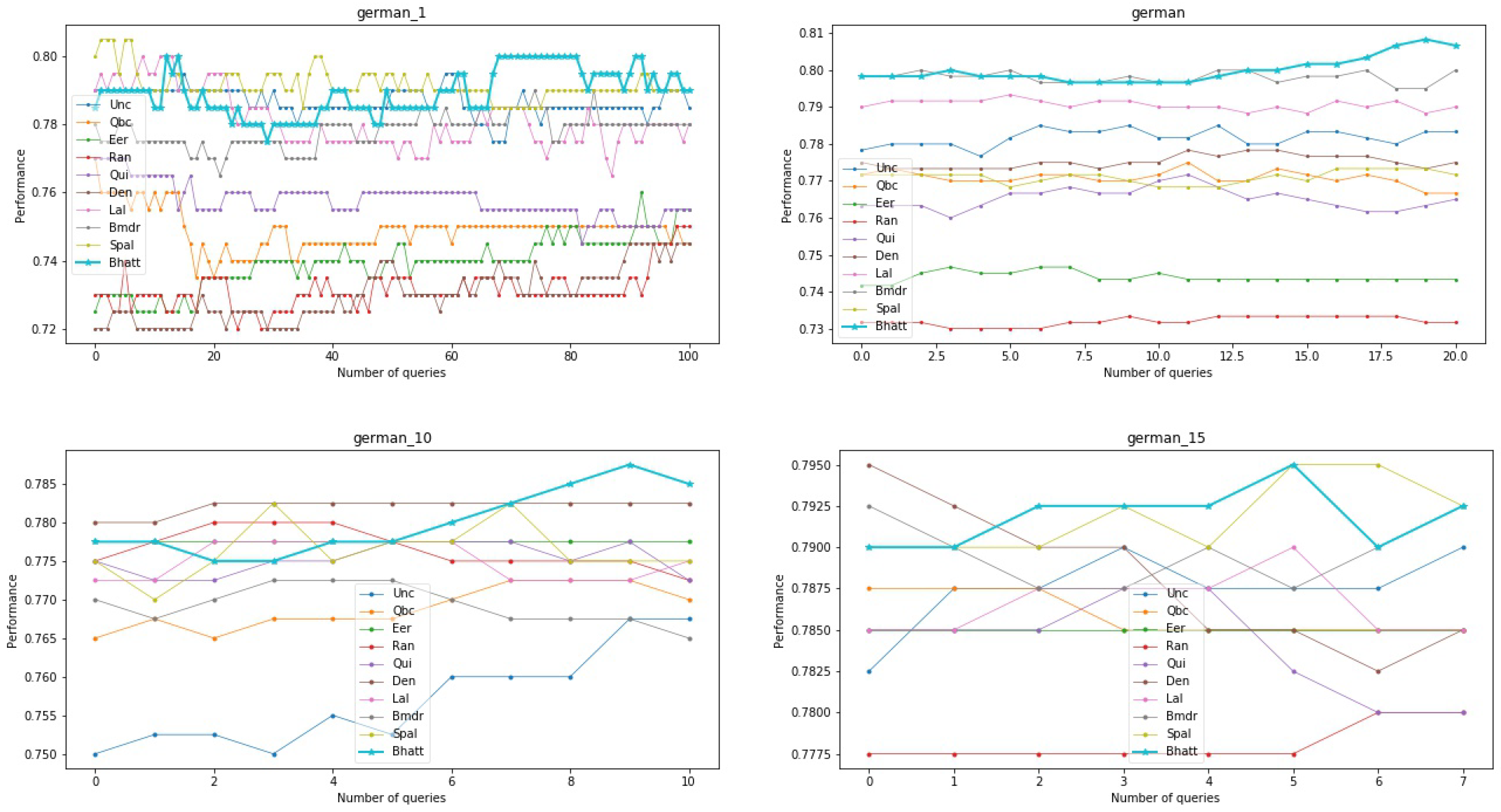
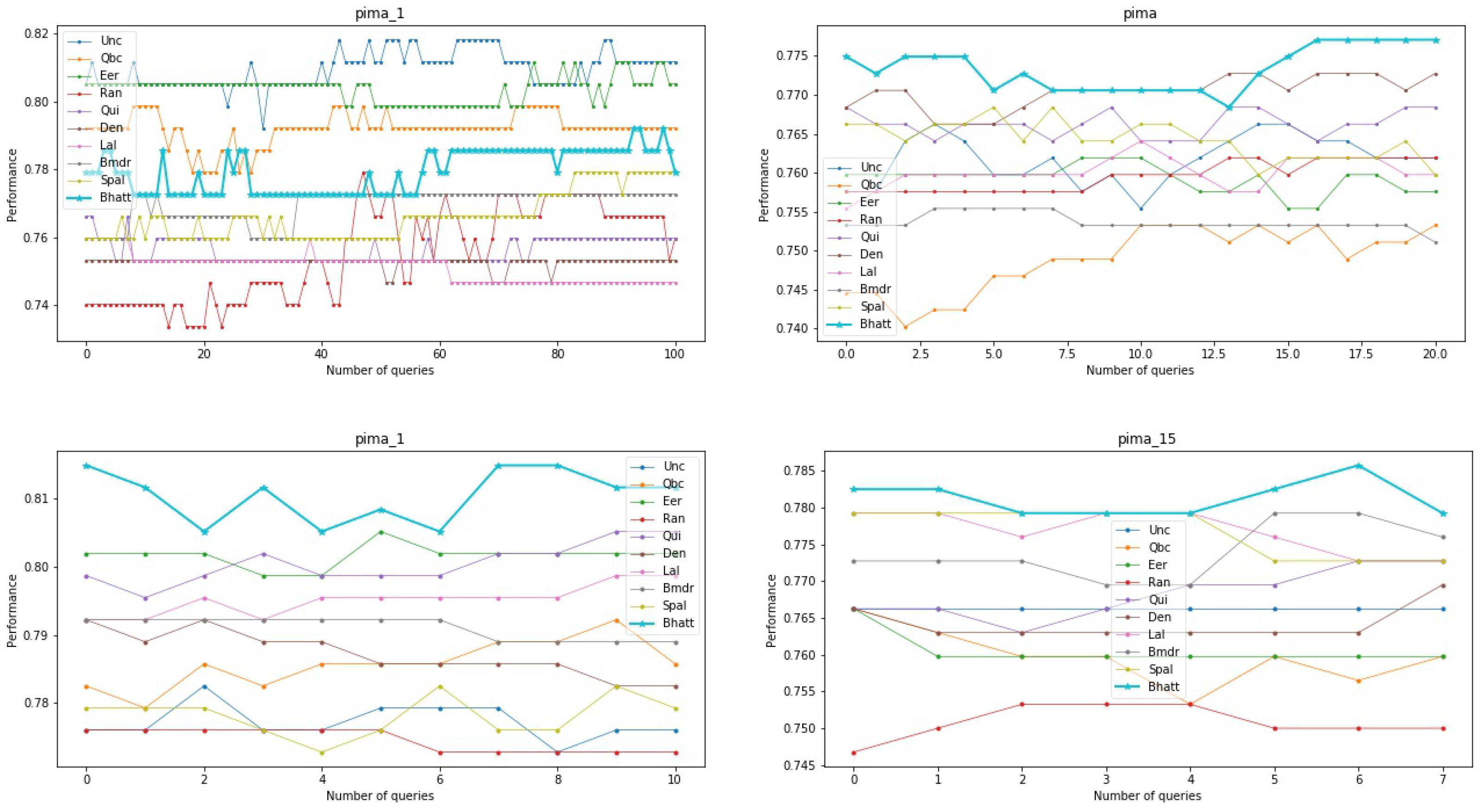
From the different methods in Figure 1 below, it can also be seen from the

Table 3. Algorithm confrontation table.

Bhatt	vs. Unc	vs. QBC	vs. EER	vs. Ran	vs. Qui	vs. Den	vs. Lal	vs. Bmdr	vs. Spal
german	85/85	80/78	86/87	70/72	88/85	76/72	77/72	80/76	77/79
breast	78/71	80/76	81/77	79/76	81/77	78/75	77/69	82/78	82/75
diabetes	76/74	77/76	77/76	72/73	73/72	77/77	80/80	76/75	74/74
heart	84/85	83/83	85/81	82/81	86/87	81/80	86/85	85/85	80/81
liver	74/73	69/68	70/69	67/67	69/69	68/65	70/69	70/72	65/64
pima	80/79	78/75	72/73	72/70	74/74	74/75	75/75	71/69	73/78

of outcome comparison that active learning with Bhattacharyya distance as a measure is dominant to a certain extent. In the case of the same query volume, we can find that the active learning accuracy measured by the Bhattacharyya distance(Bhatt) is always at the upper level, and the overall trend shows a process of rising first and then flattening.

It is not difficult to see the advantages of our method by analyzing these graphs. As shown in Figure 1, in the data sets of german, heart, and pima, our method is always at a high accuracy, and has an overall increasing trend. The common characteristics are that the fluctuation range is small and the upper limit is high, although sometimes the accuracy will decrease with the increase of the number of samples, but will soon have a greater improvement, which reflects its learning principle that combines uncertainty and representation. However, the performance of Bhattacharyya distance-based algorithm on the dataset breast is not stable, which may be caused by too little data. Compared with QBC, a query method uses information entropy as a measure and representativeness, although the upward trend of the algorithm based on the Bhattacharyya distance is weaker than the two, our algorithm is more stable. The same applies to the comparison with SPAL and BMDR, which both utilize kernel functions, our algorithm has higher accuracy, which shows that the proposed algorithm has certain advantages.

Table 3 shows the results of the active learning algorithm and other algorithms measured by the Bhattacharyya distance. In addition, 100 samples were randomly selected from the test set and the algorithm was used to predict the test samples. After multiple predictions, the average value of each group was obtained. The test predicts the correct number, and then uses this criterion for comparison. From the data in Table 3, it can be found that only 18.5% of the results are lost, and the rest are wins or draws, which shows that, in many cases, the active learning algorithm with the Bhattacharyya distance as the metric is in a different situation than other algorithms in the same situation. The results reflect its superiority in accuracy.

6.1. Batch Mode Size

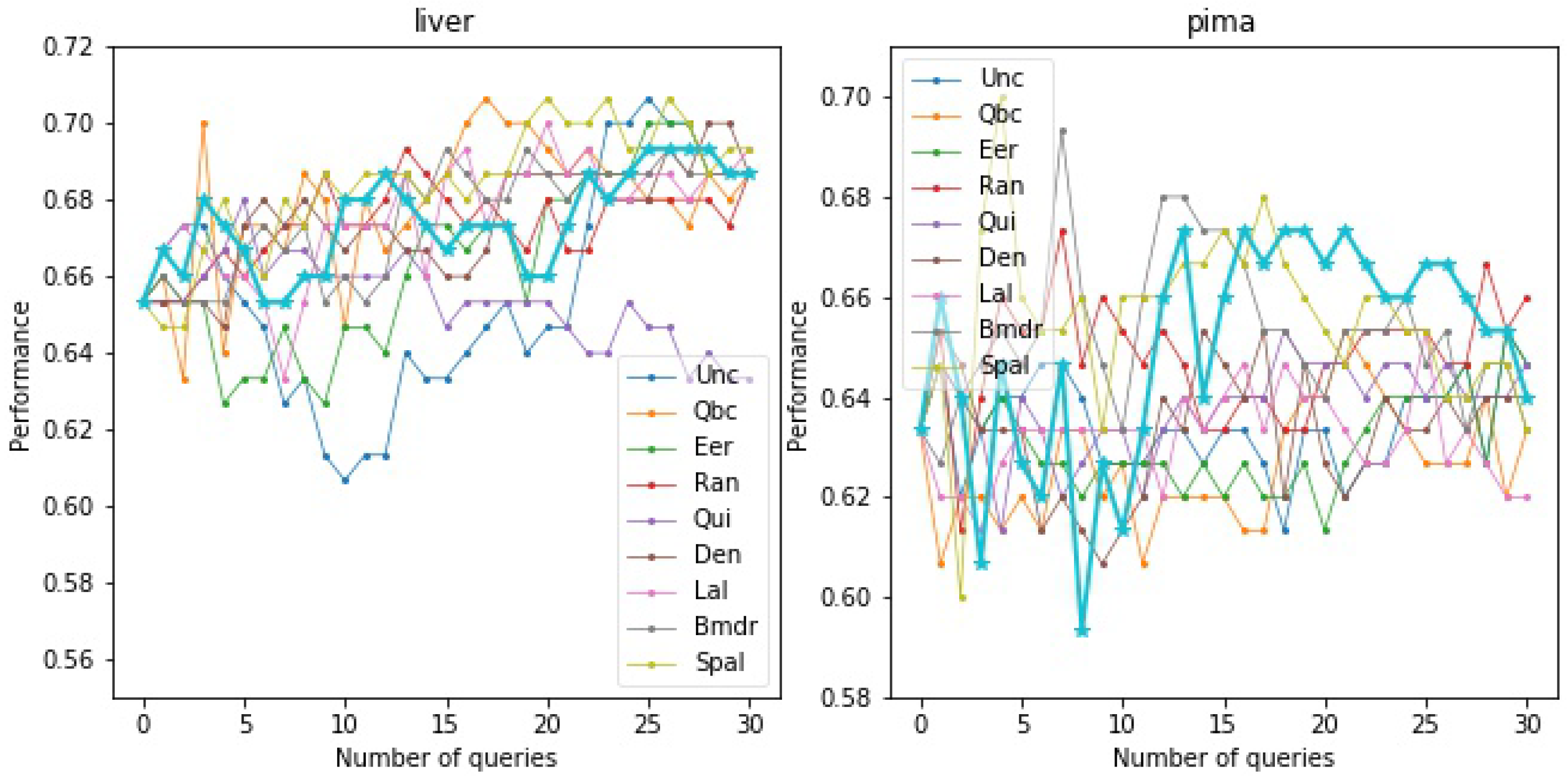
The experimental accuracy of Bhattacharyya distance active learning is shown in the following Figure 2 using a total number of queries of 30. Due to the reduction in the number of samples collected and the single sampling size of 1, the Bhattacharyya distance cannot play a leading role compared to other algorithms when the query volume is 20 and each query is 5 queries with a total of 100. The performance in the heart and liver dataset is average, but it shows a consistent upward trend on things such as german, breast, and dibetes, and outperforms most other algorithms.

By comparing the accuracy of our method with different batch sizes on the same data set, Figure 3 and Figure 4 show that the overall accuracy improvement trend is similar, but as the batch size gradually increases, the accuracy advantage gradually increases.

We can find that, when only one sample is selected at a time, our method does not have a great advantage compared with other algorithms, but when multiple samples are selected each time, it has a significant difference compared to other algorithms. It also confirms the poor performance of single sampling in Figure 2. From Figure 3 and Figure 4, we can find that, with the increase of the number of samples, the curve tends to be smooth, and the overall accuracy shows an upward trend. Compared with the BMDR that also uses the kernel function, the accuracy is better and the training speed is faster. It has been confirmed in many experiments that its stability is higher, and it has advantages over other algorithms in general.

6.2. Sensitivity of Parameters

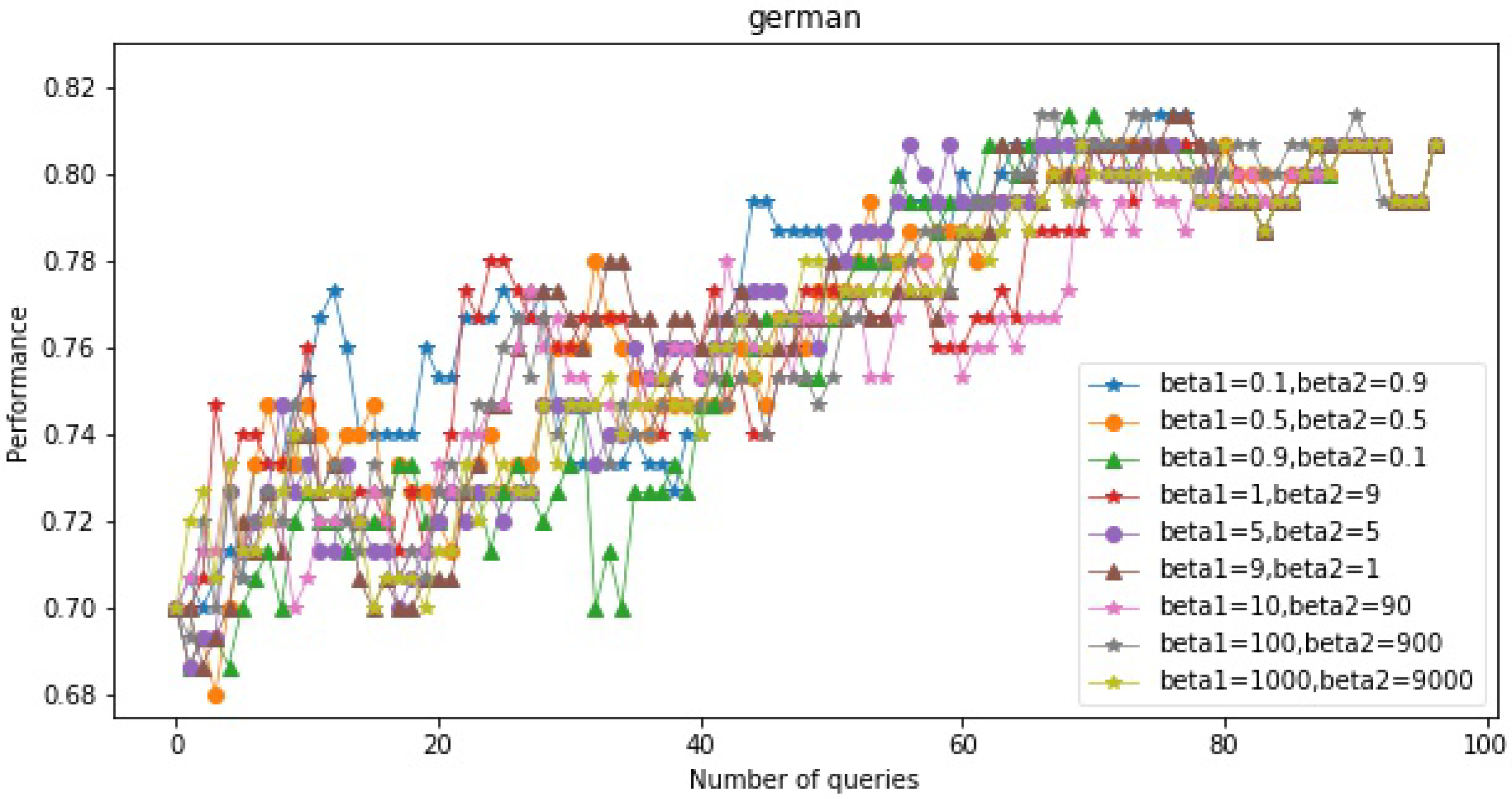
According to different learning parameters, the comparison results are shown in Figure 5 and Figure 6 below. According to the results, we can find that different data sets have sensitivity different to parameters, which may be determined by the nature of each dataset.

The result shows it is not very obvious to describe the relationship of ${\beta }_1$ and ${\beta }_2$. The overall active learning is relatively unstable under the change of parameters. From Figure 6, because the small dataset has little effect on the model prediction, the accuracy of the models with consistent parameter ratios is highly overlapped, but it can be seen that, the parameter ${\beta }_1$ is larger, the performance is better. It shows that the accuracy of our algorithm depends on the selection of the dataset and the adjustment of the parameters.

7. Conclusions

This paper proposes an active learning classification algorithm using Bhattacharyya distance as a criterion for measuring the distance of distribution. The algorithm uses the Bhattacharyya distance as the distance between the unlabeled sample set and the labeled sample set in the kernel space, so that the separability of the two distributions can be measured, and the optimal sample is selected while taking into account the representativeness and uncertainty. This ensures the accuracy and efficiency of predicting the overall data with small batches of samples.

The algorithm has two important advantages. One is that the Bhattacharyya distance represents the separability between the distributions, which can fully express the difference between the unlabeled sample and the sample to be queried. The second is that its nature does not conflict with uncertainty. The experimental results also show the correctness and the effectiveness of the active learning algorithm measured by Bhattacharyya distance. Compared with other active learning and classification algorithms, the performance of the active learning algorithm measured by Bhattacharyya distance with high accuracy.

References

- Settles, B. Active Learning Literature Survey. In Computer Sciences Technical Report 1648; University of Wisconsin: Madison, WI, USA, 2009. [Google Scholar]
- McCallumzy, A.K.; Nigamy, K. Employing EM and pool-based active learning for text classification. In Proceedings of the Proceeding International Conference on Machine Learning (ICML), Madison, WI, USA, 24–27 July 1998; Citeseer: State College, PA, USA, 1998; pp. 359–367. [Google Scholar]
- Liere, R.; Tadepalli, P. Active learning with committees for text categorization. In Proceedings of the 14th National Conference on Artificial Intelligence and 9th Conference on Innovative Applications of Artificial Intelligence, Providence, RI, USA, 27–31 July 1997; AAAI Press: Menlo Park, CA, USA, 1997; pp. 591–596. [Google Scholar]
- Wang, Z.; Ye, J. Querying discriminative and representative samples for batch mode active learning. ACM Trans. Knowl. Discov. Data (TKDD) 2015, 9, 1–23. [Google Scholar] [CrossRef]
- Lewis, D.D.; Gale, W.A. A sequential algorithm for training text classifiers. In Proceedings of the SIGIR’94, Dublin, Ireland, 3–6 July 1994; Springer: Berlin/Heidelberg, Germany, 1994; pp. 3–12. [Google Scholar]
- Sourati, J.; Akcakaya, M.; Leen, T.K.; Erdogmus, D.; Dy, J.G. Asymptotic analysis of objectives based on fisher information in active learning. J. Mach. Learn. Res. 2017, 18, 1123–1163. [Google Scholar]
- Li, M.; Sethi, I.K. Confidence-based active learning. IEEE Trans. Pattern Anal. Mach. Intell. 2006, 28, 1251–1261. [Google Scholar] [PubMed]
- Holub, A.; Perona, P.; Burl, M.C. Entropy-based active learning for object recognition. In Proceedings of the 2008 IEEE Computer Society Conference on Computer Vision and Pattern Recognition Workshops, Anchorage, AK, USA, 23–28 June 2008; IEEE: Piscataway, NJ, USA, 2008; pp. 1–8. [Google Scholar]
- Zeng, J.; Lesnikowski, A.; Alvarez, J.M. The relevance of Bayesian layer positioning to model uncertainty in deep Bayesian active learning. arXiv 2018, arXiv:1811.12535. [Google Scholar]
- Tran, T.; Do, T.T.; Reid, I.; Carneiro, G. Bayesian generative active deep learning. In Proceedings of the International Conference on Machine Learning, Long Beach, CA, USA, 10–15 June 2019; pp. 6295–6304. [Google Scholar]
- Tan, Y.; Yang, L.; Hu, Q.; Du, Z. Batch mode active learning for semantic segmentation based on multi-clue sample selection. In Proceedings of the 28th ACM International Conference on Information and Knowledge Management, Beijing, China, 3–7 November 2019; pp. 831–840. [Google Scholar]
- Du, B.; Wang, Z.; Zhang, L.; Zhang, L.; Liu, W.; Shen, J.; Tao, D. Exploring representativeness and informativeness for active learning. IEEE Trans. Cybern. 2015, 47, 14–26. [Google Scholar] [CrossRef] [PubMed] [Green Version]
- Tang, Y.P.; Huang, S.J. Self-paced active learning: Query the right thing at the right time. In Proceedings of the AAAI conference on Artificial Intelligence, Honolulu, HI, USA, 27 January–1 February 2019; Volume 33, pp. 5117–5124. [Google Scholar]
- Xu, Z.; Akella, R.; Zhang, Y. Incorporating diversity and density in active learning for relevance feedback. In Proceedings of the European Conference on Information Retrieval, Rome, Italy, 2–5 April 2007; Springer: Berlin/Heidelberg, Germany, 2007; pp. 246–257. [Google Scholar]
- Melville, P.; Yang, S.M.; Saar-Tsechansky, M.; Mooney, R. Active learning for probability estimation using Jensen-Shannon divergence. In Proceedings of the European Conference on Machine Learning, Porto, Portugal, 3–7 October 2005; Springer: Berlin/Heidelberg, Germany, 2005; pp. 268–279. [Google Scholar]
- Tong, S.; Koller, D. Active learning for parameter estimation in Bayesian networks. Adv. Neural Inf. Process. Syst. 2000, 13, 647–653. [Google Scholar]
- Bhattacharyya, A. On a measure of divergence between two multinomial populations. Sankhyā Indian J. Stat. 1946, 7, 401–406. [Google Scholar]
- Kailath, T. The divergence and Bhattacharyya distance measures in signal selection. IEEE Trans. Commun. Technol. 1967, 15, 52–60. [Google Scholar] [CrossRef]
- Bi, S.; Broggi, M.; Beer, M. The role of the Bhattacharyya distance in stochastic model updating. Mech. Syst. Signal Process. 2019, 117, 437–452. [Google Scholar] [CrossRef]
- Bartlett, P.L.; Mendelson, S. Rademacher and Gaussian complexities: Risk bounds and structural results. J. Mach. Learn. Res. 2002, 3, 463–482. [Google Scholar]
- Zhou, S.; Chellappa, R. Probabilistic distance measures in reproducing kernel Hilbert space. In SCR Technical Report; University of Maryland: College Park, MD, USA, 2004. [Google Scholar]
- Bian, Z.; Zhang, X. Pattern Recognition; Tsinghua University Press: Beijing, China, 2000. [Google Scholar]
- Roy, N.; McCallum, A. Toward optimal active learning through monte carlo estimation of error reduction. ICML Williamstown 2001, 2, 441–448. [Google Scholar]
- Huang, S.J.; Jin, R.; Zhou, Z.H. Active learning by querying informative and representative examples. Adv. Neural Inf. Process. Syst. 2010, 23, 1936–1949. [Google Scholar] [CrossRef] [PubMed] [Green Version]
- Ebert, S.; Fritz, M.; Schiele, B. Ralf: A reinforced active learning formulation for object class recognition. In Proceedings of the 2012 IEEE Conference on Computer Vision and Pattern Recognition, Providence, RI, USA, 16–21 June 2012; IEEE: Piscataway, NJ, USA, 2012; pp. 3626–3633. [Google Scholar]
- Fang, M.; Li, Y.; Cohn, T. Learning how to active learn: A deep reinforcement learning approach. arXiv 2017, arXiv:1708.02383. [Google Scholar]
Figure 1.
The comparison of different performance on different datasets, and it can be seen that the active learning algorithm with Bhattacharyya distance as the measurement still maintains a high learning accuracy, and shows a high-speed upward trend as the number of query samples increases.
Figure 2.
Performance on different datasets with query size = 30; it can be seen that, in the case of a single query, although the start is relatively slow, it can quickly improve in most data sets. In addition, it performs better than most data sets. These situations show that active learning with Bhattacharyya distance as a measure is superior in comparison with the same type of active learning. However, there are still relatively unstable situations in some data sets, indicating that the algorithm may need further optimization in specific occasions.
Figure 3.
Performance comparison on the German dataset, compared with single active learning; batch active learning is more efficient while maintaining higher accuracy.
Figure 4.
Performance comparison on the Pima dataset, and it can be found that, when batch_size = 5, the performance is the best, and the rising trend of accuracy improvement is also the most obvious, which is suitable for the application of actual scenes.
Figure 5.
Performance comparison about different parameters on German dataset.
Figure 6.
Performance comparison about different parameters on Breast dataset.