Agglomeration Regimes of Particles under a Linear Laminar Flow: A Numerical Study

Abstract

In this work, a combined smoothed particle hydrodynamics and discrete element method (SPH-DEM) model was proposed to model particle agglomeration in a shear flow. The fluid was modeled with the SPH method and the solid particles with DEM. The system was governed by three fundamental dimensionless groups: the Reynolds number Re (1.5~150), which measured the effect of the hydrodynamics; the adhesion number Ad (6 × 10⁻⁵~6 × 10⁻³), which measured the inter-particle attraction; and the solid fraction α, which measured the concentration of particles. Based on these three dimensionless groups, several agglomeration regimes were found. Within these regimes, the aggregates could have different sizes and shapes that went from long thread-like structures to compact spheroids. The effect of the particle–particle interaction model was also investigated. The results were combined into ‘agglomeration maps’ that allowed for a quick determination of the agglomerate type once α, Re, Ad were known.

1. Introduction

Particle agglomeration exists widely in both nature and industry. In the mining industry, for instance, particle aggregation in solid–liquid separation is beneficial for the acceleration of slurry dewatering and improving thickening and filtration operations [1]. In the pharmaceutical sector, granulation for compression blends is also aided by agglomeration [2]. However, agglomeration can also be detrimental as it causes clogging of microchannels in microfluidic devices [3], speeds up the erosion of turbine blades in gas turbine engines [4,5] and reduces the efficiency of drug particle delivery [6]. Therefore, either to promote it or to avoid it, a deep understanding of particle agglomeration is indispensable for optimizing particulate processing in both water and air.

According to many experimental investigations, the number of particles in an aggregate typically varies as an exponential function of the radius of gyration of the aggregates, where the exponent of the function is referred to as the aggregates’ fractal dimension [7,8,9]. The fractal dimension’s value is determined by the mechanism through which the aggregate was generated and the stage at which it was formed. Typical values of fractal dimension are in the range of roughly 1.5 to 3.0 [10]. The fractal dimension influences the aggregate’s material characteristics, such as its elastic and shear moduli [11,12,13]. The force network of aggregate is affected by its fractal structure, which impacts the shear stress required to cause aggregate fragmentation [14,15,16,17,18].

Although there is extensive experimental research on particle agglomeration, the dynamic behavior of primary particles smaller than roughly 10 µm is difficult to image. Therefore, numerical simulations of particle agglomeration in multiphase flows are now widely used to provide an insight into particle behaviour. Shear effects have been extensively investigated in previous numerical studies on particle agglomeration [19,20,21]. By using an Eulerian–Lagrangian approach, Hellestø et al. [21] numerically explored the agglomeration of cohesive particles in a simple shear flow. They found that, when the hydrodynamic forces dominated compared to adhesion forces, the steady state aggregate diameter increased with a decreasing shear rate. Another essential consideration was the effect of inter-particle interactions on aggregate structure. Cohen [22] explored the influence of particle interaction surface energy on aggregate structure. As expected, it was found that high surface energy corresponded to the formation of large aggregates.

Recently, some researchers have used an Eulerian–Lagrangian (a combined computational fluid dynamics (CFDs) and DEM) method to investigate agglomeration or deagglomeration in both laminar and turbulent flows [20,21,23,24,25,26,27,28]. These studies only accounted for momentum exchange between the fluid–solid phases and not for the physical presence of the particles in the fluid (the particles were ‘transparent’ to the flow). In this paper we coupled two discrete particle methods, SPH [29] and DEM [30], to model all interactions (i.e., fluid–fluid, fluid–particle and particle–particle) occurring in the system. The SPH method has the advantage of utilizing a Lagrangian meshless technique, which made detecting the interface between particles or aggregates simple, avoiding the complications of tracking the interface location [31,32]. This novel SPH-DEM approach has been widely validated for a broad range of complex fluid–solid interaction problems [33,34,35,36]. Moreover, it was used and also validated by Rahmat et al. [37], but they used an overly simplistic representation of the particle–particle interaction. We improved this here by using two of the most common adhesion contact models: the Johnson–Kendall–Roberts (JKR) [38] and the Derjaguin–Muller–Toporov (DMT) [39] models. To our knowledge, the effect of these two popular contact models on agglomeration types has not been investigated. The proposed SPH-DEM model was used to investigate the effect of various important parameters on particle agglomeration in a shear flow, such as the Reynolds number, adhesion number and the solid volume fraction.

2. Methods

In this study, we used discrete multiphysics (DMP) for modeling solid–liquid flows. In general, DMP can combine several particle methods together (for instance SPH, coarse grained molecular dynamics and DEM). In this paper, we combined SPH for the liquid phase and DEM for the solid particles [40]. Only a brief introduction to both SPH and DEM is provided since the methods were described in earlier work [29,30].

In general, all particle methods solve the Newton equation of motion:

$$m_i\frac{d{v}_i}{dt}=m_i\frac{d^2{r}_i}{d{t}^2}={\displaystyle \sum }_{i \ne j}{F}_{i,j}+{\displaystyle \sum }{F}_E$$

(1)

where m_i is the mass of particle i, r_i its position, v_i its velocity, F_i,j is the interparticle force between particle i and j and F_E is an external force. This equation is common to all particle methods; the difference between SPH and DEM lies in the term F_i,j.

2.1. SPH (Liquid Phase)

Smoothed particles hydrodynamics (SPH) is a meshless particle-based algorithm, proposed by Lucy, Gingold and Monaghan in 1977 [31,41]. Here, it was utilized to simulate the solid–fluid two-phase flow. Individual particles in the SPH domain were given properties such as velocity, position, density and pressure, which were updated at every time step.

The SPH method discretizes the Navier–Stokes’s equation into a form that is comparable with Equation (1) [29]:

$$F_i=m_i\frac{d{v}_i}{dt}=-{\displaystyle \sum }_j{m}_i{m}_j\left(\frac{p_i}{{\rho }_i^2}+\frac{p_j}{{\rho }_j^2}+{\mathsf{\Pi }}_{ij}\right){\nabla }_i{W}_{ij}$$

(2)

where F_i is the sum of the forces applied to the particle i, m_j is the mass of particle j, ${\rho }_i$ is the density of particle i, p is the pressure. W is the smoothing kernel function that defines how the inter-particle interaction changes with their distance r_ij = r_i − r_j. ${\mathsf{\Pi }}_{ij}$ is the artificial viscosity. For W, the Lucy kernel is used herein [42]:

$$W(r<h)=\frac{105}{16\pi h^3}\left[1+3\frac{r}{h}\right]{\left[1-\frac{r}{h}\right]}^3$$

(3)

where $h$ is the smoothing length and indicates how far each particle is influenced by the nearby particles.

The artificial viscosity below is used [42]:

$${\mathsf{\Pi }}_{ij}=-\beta h\frac{c_i+c_j}{{\rho }_i+{\rho }_j}\frac{v_{ij}\cdot r_{ij}}{r_{ij}^2+ϵh^2}$$

(4)

where $\beta$ is a dimensionless factor influencing the dissipation strength, $c_i$ and $c_j$ are the sound speeds of particles i and j, respectively, and $ϵ=$ 0.01 prevents singularities when particles are relatively close to each other.

An equation of state allows the calculation of the pressure p as a function of local density ρ [43]. In this research, the Tait equation [29] is used:

$$p=\frac{c_0^2{\rho }_0}{7}\left[{\left(\frac{\rho }{{\rho }_0}\right)}^7-1\right]$$

(5)

where $c_0$ is a reference speed and ρ₀ is a reference density.

2.2. DEM (Solid–Solid Interaction)

Equation (1) was also used to simulate the interaction between two real particles. In this case, the DEM for solid–solid interactions was used. DEM particles are not point particles. Each solid particle i is subjected to the force and moment of the other solid particles in contact with it. For this reason, we needed to solve Equation (1) in conjunction with the equation for the conservation of angular momentum:

$$I_i\frac{d{\omega }_i}{dt}={\displaystyle \sum }_{i \ne j}{R}_i F_{i,j}$$

(6)

where I_i, ω_i, R_i and F_i,j are the moment of inertia, the angular velocity, the radius of the particle i and the inter-particle force, respectively.

Here, the inter-particle forces F_i,j are the contact forces and include (i) the non-adhesive elastic contact after a particle–particle collision and (ii) the adhesive contact between two spherical particles.

The non-adhesive elastic contact can be described by Hertzian theory [44]. In the Hertz model, the normal elastic force is computed as follows:

$$F_{ne,Hertz}=k_n{R}_{eff}^{1/2}{\delta }_{ij}^{3/2}n$$

(7)

where $R_{eff}=\frac{R_i{R}_j}{R_i+R_j}$ is the effective radius, which, for simplicity, is denoted as $R$ from here on. $k_n$ is the spring constant. ${\delta }_{ij}=R_i+R_j-\left|r_{ij}\right|$ is the particle overlap, R_i, R_j are the radius of particle i and j, respectively, and r_ij = |r_j − r_i| is the vector separating the two particle centers and n = r_ij/r_ij. Since the elastic modulus and the shear modulus of the two particles were the same in this study, $k_n=4/3E_{eff}$. Here,

$$E_{eff}=E={\left(\frac{1-{\nu }_i^2}{E_i}+\frac{1-{\nu }_j^2}{E_j}\right)}^{-1}$$

(8)

where $E_{eff}$ is the effective Young’s modulus, with ${\nu }_i,{\nu }_j$ and $E_i$, $E_j$, the Poisson ratios and Young’s modulus of the particles of types $i$ and $j$.

The deformations become more difficult when adhesion forces are introduced. The Johnson–Kendall–Roberts (JKR) theory [38] and the Derjaguin–Muller–Toporov (DMT) theory [39] are two modern theories of adhesion contact mechanics between two spherical particles. The DMT model assumes that, during particle contact, attractive forces do not change the surface profile [39]. The assumption of the JKR model is that adhesion only occurs inside a flattened contact zone [38]. DMT theory is applicable to very small and hard bodies with low surface energies, whereas JKR theory better describes easily deformable, large bodies with high surface energies [45]. In this study, to make the results more general, both models were used and compared.

In the DMT model, the normal, elastic force is simply Hertzian with an additional attractive cohesion term:

$$F_{ne,dmt}=\left(\frac{4}{3}E R^{1/2}{\delta }_{ij}^{3/2}-4\pi \gamma R\right)n$$

(9)

where $\gamma$ is surface energy of solid particles.

In the JKR model, the normal, elastic force is computed as:

$$F_{ne,jkr}=\left(\frac{4E{a}^3}{3R}-2\mathsf{\pi }{a}^2\sqrt{\frac{4\gamma E}{\pi a}}\right)n$$

(10)

where a is the radius of the contact zone related to the overlap δ based on the following:

$$\delta =a^2/R-2\sqrt{\pi \gamma a/E }$$

(11)

The following damping component was also needed to add to the normal force:

$$F_{n,damp}=-{\eta }_n{v}_{n,rel}$$

(12)

where $v_{n,rel}=\left(v_j-v_i\right)\cdot nn$ is the component of relative velocity along $n$ and ${\eta }_n$ is the normal damping factor.

The damping term used a damping viscoelastic model [44]. Therefore, the normal damping factor is given by the following:

$${\eta }_n={\eta }_{n0}a{m}_{eff}$$

(13)

where ${\eta }_{n0}$ is the normal damping coefficient, $a$ is the contact radius, given by (a) $a=\sqrt{R\delta }$ for the DMT model and (b) $\delta =a^2/R-2\sqrt{\pi \gamma a/E}$ for the JKR model. $m_{eff}=m_i{m}_j/\left(m_i+m_j\right)$ is the effective mass.

The combination of the elastic and damping elements yields the total normal force:

$$F_n=F_{ne}+F_{n,damp}$$

(14)

Apart from the normal contact force, the tangential contact force was also required. Based on the Mindlin tangential contact model [46,47], the tangential force is given by the following:

$$F_t=-\min \left({\mu }_t{F}_{n0}, \left|-k_{t}a\xi +F_{t,\mathit{damp}}\right|\right)t$$

(15)

Here, ${\mu }_t$ is the tangential friction coefficient. $k_t$ is the tangential stiffness coefficient. $\xi$ is the tangential displacement collected over the contact’s full duration.

$F_{n0}$ is the normal force value given by the following:

$$F_{n0}=\left|F_{ne}+2F_{\mathrm{pull-off} }\right|$$

(16)

where $F_{\mathrm{pull-off} }=3\pi \gamma R$ for the JKR model and $F_{\mathrm{pull-off} }=4\pi \gamma R$ for the DMT model.

The tangential damping force $F_{\mathrm{t},\mathrm{damp}}$ is computed as follows:

$$F_{\mathrm{t},\mathrm{damp}}=-{\eta }_t{v}_{t,rel}$$

(17)

where ${\eta }_t$ is the tangential damping prefactor and is calculated by scaling the normal damping ${\eta }_n$, here ${\eta }_t=-{\eta }_n$was used. $v_{t,rel}$ is the relative tangential velocity at the point of contact.

2.3. Solid–Fluid Interactions

To simulate the fluid–solid interaction, the forces between fluid and solid particles must be defined. These forces must guarantee no slips, no penetration and continuity of stresses between the fluid–solid interface. These conditions [40] are usually expressed in continuum mechanics as follows:

$$\left(\frac{\partial }{{\partial }_t}u-v\right)· n=0 \left(\mathrm{no} \mathrm{penetration}\right)$$

(18)

$$\left(\frac{\partial }{{\partial }_t}u-v\right)\times n=0\left(\mathrm{no} \mathrm{slip}\right)$$

(19)

$${\sigma }_{ s}n={\sigma }_{ f}\left(-\left|r\right|\right) \left(\mathrm{continuity} \mathrm{of} \mathrm{stresses}\right)$$

(20)

where v is the fluid velocity, $u$ the displacement of the solid, n the direction normal to the boundary and ${\sigma }_{ f}$ and${\sigma }_{ s}$ are the fluid and solid stresses, respectively.

These conditions needed to be ‘translated’ in terms of forces F_i,j in order to be introduced in the DMP model.

In SPH simulations, non slip conditions at the rigid walls are approximated by modeling the walls as layers of ‘frozen’ (i.e., forces are calculated normally, but positions are not updated) fluid particles. Here, this approach was used between the walls and the fluid. However, it could not be used between the fluid particles and the solid particles of the agglomerates because agglomerates needed to be free to move into the flow. Nevertheless, if the fluid particles ‘saw’ the solid particles as fluid particles, we had the same situation that occurs at rigid SPH walls, but without restricting the motion of the solid particles. In other words, to achieve non slip conditions, the fluid saw the agglomerates as moving rigid boundaries with the same shape of the agglomerate.

No penetration was achieved by adding repulsive forces between the solid and liquid particles. Generally, SPH also includes repulsive forces to reduce particle overlap (e.g., Equation (2)). Usually, these forces are not strong enough to fully remove overlaps between solid and liquid particles and, therefore, additional repulsive forces are necessary. According to the flow, different types of additional repulsive forces were used, see for instance [48,49,50,51]. In this present study, however, velocities were not particularly high and no additional force was required.

Finally, the continuity of stresses in particle methods was automatically enforced by Equation (1). More details on boundary solid –liquid conditions in DMP can be found in the literature (e.g., [52,53,54]).

2.4. Software

In 1993, Steve Plimpton created a large-scale atomic/molecular massively parallel simulator (LAMMPS) [55]. This open-source software LAMMPS was used for the simulations of the DMP model. Many researchers have enhanced and expanded LAMMPS since its initial release, incorporating mesh-free computational methods such as DEM and SPH, as well as others [42,56]. LAMMPS is a molecular dynamics (MD) algorithm that simulates groups of particles in solids, liquids and gases. Using different boundary conditions and inter-particle potentials, it can simulate microscopic, mesoscopic or macroscopic systems. Generally, LAMMPS solves Newton’s motion equations about a group of interaction particles. To meet certain research needs, custom features in the LAMMPS source code can be implemented by using LAMMPS input script commands. Then information, such as the position and velocity of the particles, is outputted. However, LAMMPS could not carry out in-depth analysis of the simulation and could not visualize and plot our output data; however, this could be performed by Ovito software [57]. This powerful software played an important role in obtaining scientific insights from the data. Without the appropriate visualization and analysis software package, key information would have stayed unknown and unavailable.

2.5. Dimensionless Analysis

Based on the Buckingham π theorem, a physically relevant equation containing n physical variables could be reformulated in terms of a collection of p = n − k dimensionless parameters ${\Pi }_1,{\Pi }_2,\dots {\Pi }_p$, where k is the number of physical dimensions involved.

In the case under consideration, the results were best expressed as a mathematical function f of the type

$$f\left({\langle n\rangle }_t,\gamma ,\alpha ,d, U, H, \mu , \rho , {\rho }_P, t\right)=0$$

(21)

where all the variables and their respective physical units are listed in

Table 1. Variables for dimensional analysis.

	Variable	Units	Description
(1)	${\langle n\rangle }_t$	-	Number of particles in the average aggregate after time t, namely average aggregate size, which is the average overall aggregates after time t when the steady state was reached
(2)	γ	kg s−2	Surface energy
(3)	α	-	Solid volume fraction
(4)	d	m	Particle diameter
(5)	$U$	m s−1	Wall velocity (Table 2)
(6)	H	m	Domain size in the y direction (Figure 1)
(7)	µ	kg m−1 s−1	Viscosity of the liquid
(8)	ρ	kg m−3	Density of the liquid
(9)	ρp	kg m−3	Density of the solid particle
(10)	t	s	Agglomeration time

. Since there were 10 variables and 3 units (kg, m, s), Equation (21) could be rewritten based on the 7 dimensionless groups. However, in the case considered, the fluid mechanical properties µ and ρ of the fluid (water), the size of the computational domain H and the agglomeration time t were fixed. Therefore, these parameters were constant, and we only needed 4 dimensionless groups that could be associated with a relation of the type

$${\langle n\rangle }_t=\phi \left(\alpha , Re,Ad\right)$$

(22)

These dimensionless groups can be defined in different ways. ${\langle n\rangle }_t$ and $\alpha$ are already dimensionless, Re is the Reynolds number defined as

$$Re=\frac{\rho UH}{\mu }$$

(23)

and Ad the adhesion number

$$Ad=\frac{\gamma d{\rho }_P}{{\mu }^2}$$

(24)

Re, as usual, represents the ratio between inertial and viscous forces in the fluid; Ad represents the ratio between the interparticle adhesion forces and the viscous forces. However, given that ρ, H and µ were constant, it is probably easier in the next sections to interpret Re and Ad simply as a dimensionless wall velocity and a dimensionless a surface energy, respectively.

Based on this dimensionless analysis, instead of carrying out a parametric study to understand how ${\langle n\rangle }_t$ changed with all parameters in Table 1, the same information could be provided by carrying out a parametric study to understand how ${\langle n\rangle }_t$ changed with $\alpha$, Re and Ad.

3. Results

3.1. Simulation Setup

Figure 1 shows the computational domain and the initial status at zero time. Four particle types were included in the system. The fluid particles (green) were located between a top wall (yellow) and a bottom wall (blue, stationary) along the y direction. To generate shear flow in the channel, the top wall, along the x direction, had constant velocity U. The solid particles (red) were randomly located within the fluid domain based on their volume fractions. Boundary conditions along the x and z directions were periodical. The Reynolds number Re was varied by changing the values of the velocity U of the top wall.

To investigate how solid particle aggregates evolved, simulations were performed under different parameters, as shown in

Table 2. Parameters used in the simulation of the structural evolution of solid particle agglomerates.

Fluid density	1000 kg/m3
Fluid dynamic viscosity	0.001 Pa·s
Solid particle diameter	6 µm
Particle density	1000 kg/m3
Number of SPH fluid particles	526–601 (depending on solid volume fraction: 1.2–4.2%)
Number of solid particles	47–157 (depending on solid volume fraction: 1.2–4.2%)
Number of wall particles	980
Mass of each fluid particle	1.4 × 10−12 kg
Mass of each solid particle	1.1 × 10−13 kg
Initial distance between fluid particles, sc	1 × 10⁻5–2 × 10⁻5 m
Smoothing length h	2.6 × 10⁻5–5.2 × 10⁻5 m
Sound speed c0	1 m/s
Reynolds number	1.5–150
Surface energy density	1.1 × 10−6–1.1 × 10−8 J/m2
Solid volume fraction	1.2–4.2%
Poisson’s ratio	0.33
Time step	5.7 × 10−6 s
Computational domain along x, y and z direction in order: W × H × L	7.5 × 10−5 m × 2 ×10−4 m × 7.5 × 10−5 m

.

3.2. Preliminary Results

To produce fluid resolution-independent results, how the number of solid particles in the average aggregate ${\langle n\rangle }_t$ changed with fluid resolution was investigated. In these preliminary results, the primary solid particles always had the same size and only the fluid particle resolution was increased.

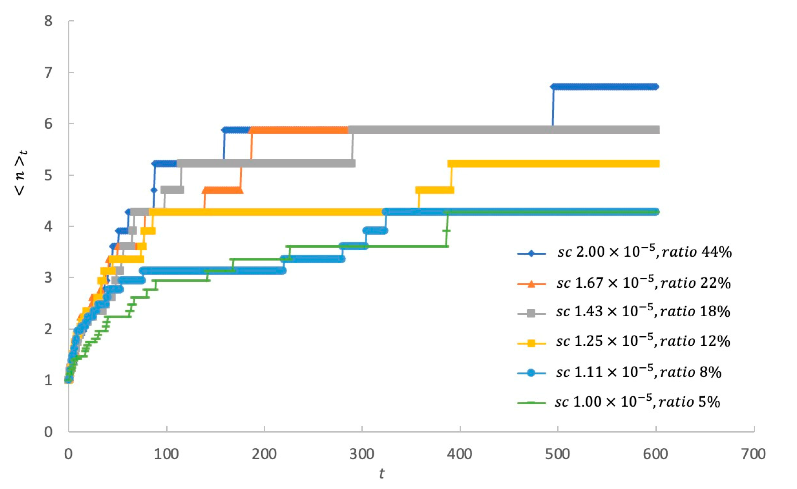
The evolution of average aggregate size with different fluid resolutions (ratio between fluid and solid particles) is shown in Figure 2. The critical factor in this resolution study was the number of fluid particles that surrounded a solid agglomerate. If there were too few, it was difficult to resolve the fluid dynamics around the agglomerate in sufficient detail. As primary particles agglomerated, the size of the agglomerate increased. Therefore, as the simulation progressed the limitation of an inadequate initial resolution tended to decrease. For this reason, only the results during the initial phase when the agglomerate size was relatively small were compared. Figure 2 shows that the results did not change considerably when the initial distance between fluid particles, sc was decreased from 1.11 × 10⁻⁵ m to 1.00 × 10⁻⁵ m, which corresponded to a decrease in the ratio between the number of solid and liquid particles from 8% to 5%. Given the random position of the initial solid particle distribution, the agglomeration profiles at higher resolutions were not expected to converge to exactly the same curve. Hence, considering the balance between accuracy and computational costs, sc = 1.11 × 10⁻⁵ m was selected as the reference fluid particle resolution and was employed throughout this study, unless stated otherwise. At the very beginning of the simulation, when only small agglomerates were in the fluid, the fluid around the particles was probably still under resolved, but as the agglomerate grew this problem fixed itself. Therefore, the goal of the resolution analysis was to establish a resolution whose initial underperformance did not sensibly affect the later stages of the simulation.

3.3. Particle Agglomeration

Simulations were performed with different values of Reynolds number, adhesion number and solid particle volume fraction to investigate the structural behavior of solid aggregates.

3.3.1. Effect of Re and Ad

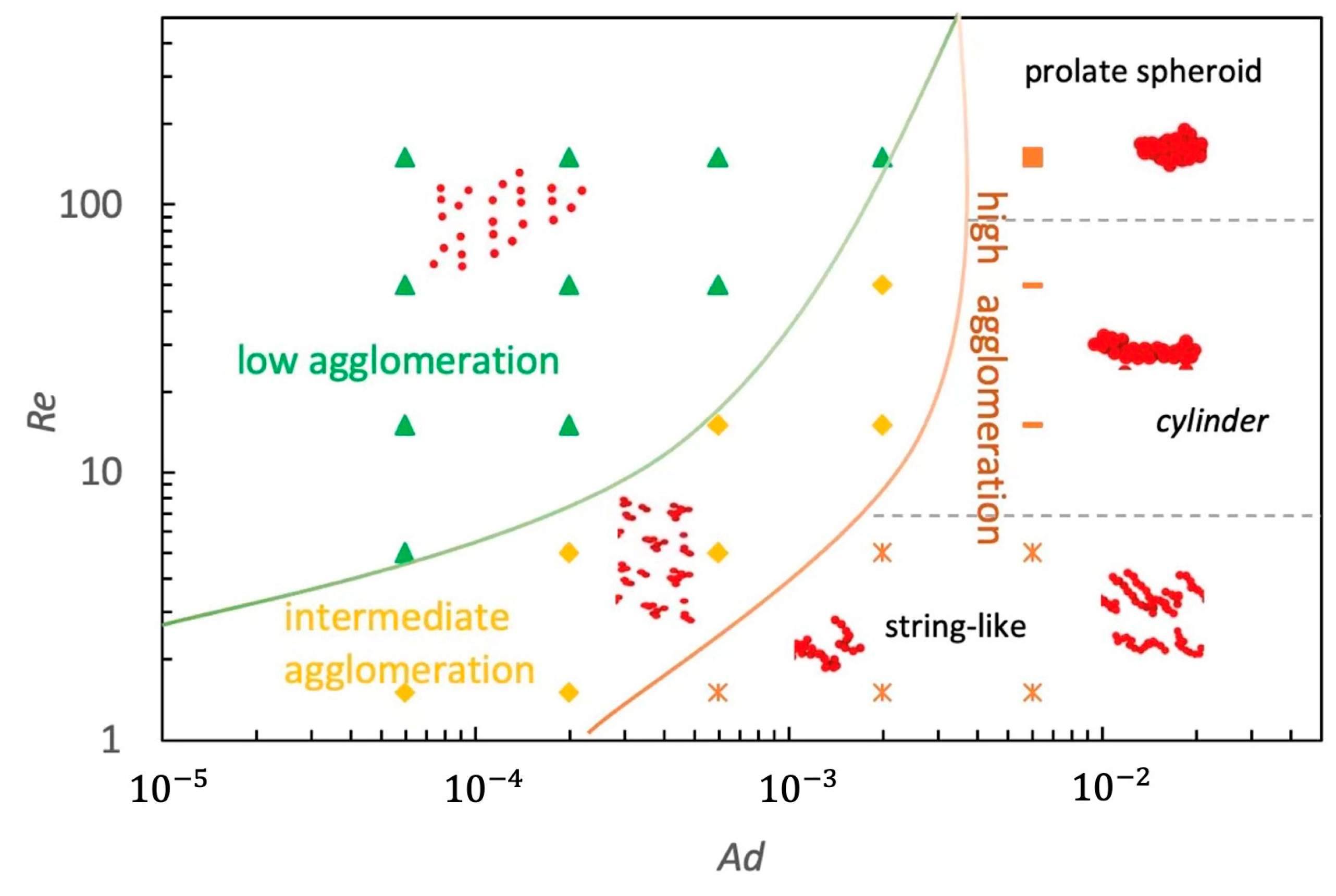
In the simulations, the average aggregate size attained a steady size after initial growth. This steady state could be reached in three different ways, depending on whether shear or adhesion dominated, or if both mechanisms were at play. The first occurred when shear prevailed. When particles have low surface energy, there is little agglomeration. Even when small agglomerates formed, they were quickly broken apart by the hydrodynamic forces. This led to many dispersed primary particles at the steady state. The second occurred when agglomeration prevailed. Aggregates stopped growing only after they cleaned the entire surrounding area and there were no particles left for further agglomeration. This led to a single spheroidal aggregate within the computational domain. The final mechanism occurred when agglomeration and fragmentation reached a dynamic equilibrium that resulted in a constant average size, but with shapes ranging from squashed spheres to strings of primary particles. Figure 3 shows several aggregates forming at a solid volume fraction of 4.2% for different values of Re and Ad. At large adhesion numbers, adhesion forces were dominant and agglomeration prevailed. At small adhesion numbers, solid particles do not stick to each other, leading to very dispersed systems.

The simulations also showed that dispersed systems tended to concentrate particles towards the center of the channel, while large aggregates were preferentially located near the walls. This observation was consistent with previous studies dedicated to the inertial migration of rigid spheres in shear flow and it was the result of competition between wall-induced and shear-gradient-induced lift forces [58,59,60,61,62].

Figure 3 gives a visual representation of the aggregates;

Table 3. Relative average aggregate size n* for different Reynolds Re and adhesion Ad numbers at a solid particle volume fraction 4.2%.

	Ad	6 × 10−5	2 × 10−4	6 × 10−4	2 × 10−3	6 × 10−3
Re
150		0.00762	0.00765	0.00767	0.00857	0.50000
50		0.00723	0.00736	0.00785	0.01827	1.00000
15		0.00834	0.01024	0.02104	0.07389	0.50000
5		0.01097	0.02177	0.07062	0.14729	0.39706
1.5		0.02921	0.07343	0.16667	0.20000	1.00000

and

Table 4. Scaled average radius of gyration Rg* for different Reynolds Re and adhesion Ad numbers at a solid particle volume fraction 4.2%.

	Ad	6 × 10−5	2 × 10−4	6 × 10−4	2 × 10−3	6 × 10−3
Re
150		0.15	0.09	0.12	0.20	2.98
50		0.12	0.13	0.13	0.55	4.02
15		0.21	0.35	1.28	2.00	4.92
5		0.41	1.20	2.15	3.80	7.57
1.5		1.39	2.37	4.66	5.77	17.35

provide a quantitative analysis. Table 3 shows the relative average aggregate size at the steady state defined as

$$n^{*}= \frac{{\langle n\rangle }_t}{N}$$

(25)

where N is the total number of primary solid particles at the steady-state for different Re and Ad at α = 4.2%.

Table 4 shows the scaled average radius of gyration at the steady state defined as

$$R_g^{*}= \frac{2\langle R_g\rangle }{d}$$

(26)

where d is the diameter of a solid particle; R_g is the radius of gyration of each aggregate and is computed by the formula

$$R_g= \sqrt{\frac{1}{M} {\displaystyle \sum }_i{m}_i{\left(r_i-r_{cm}\right)}^2 }$$

(27)

where M is the total mass of each aggregate, r_cm is the center-of-mass position of each aggregate and the sum is over all particles in each aggregate.

R_g* = 0 is a single primary particle, while a dimer has R_g* = 1. As R_g* increased, the number of branches of the aggregate shape increased and it became more irregular.

The information from Figure 3 and Table 3 and Table 4 are combined into a single figure (Figure 4) that shows how, based on Re and Ad, the system could be subdivided into different regimes.

Figure 4 shows three different regimes, i.e., low (n* < 0.015), intermediate (0.015 < n* < 0.1) and high (n* > 0.1) agglomeration. Low agglomeration occurred where shear prevailed; intermediate agglomeration occurred where agglomeration and fragmentation reached a dynamic equilibrium; high agglomeration occurred where agglomeration prevailed. Based on the aggregate shape, the high agglomeration area could be further subdivided into three regions. In the high-Re region the aggregate shape was a prolate spheroid. In the middle-Re region, the aggregates were cylindrical. Finally, at low-Re the shape was string-like.

3.3.2. Effect of α

The same procedure was used to identify the agglomeration regimes for a different volume fraction, α = 2.4%.

Figure 5 also presents three agglomeration regimes, i.e., low, intermediate and high agglomeration. The major difference between Figure 4 and Figure 5 is in the low-Re region of the high agglomeration area. While at α = 4.2% a single long string formed, at α = 2.4% there several shorter strings. Due to the lower density, there were fewer particles for agglomeration and the shorter strings did not merge into a single chain.

3.3.3. Effect of the Adhesion Model

Up to this point, the results presented have been based on the JKR adhesion model (Equation (10)). In this section, the simulations were performed with the DMT model (Equation (9)) for comparison. Figure 6 shows the agglomeration regimes obtained with the DMT model at α = 4.2%. In general, it shows a similar map to the JKR model. In the high agglomeration area, the JKR model tended to generate branched aggregates or particle chains while the DMT model predicted relatively regular (more compact with fewer or no branches at all) small aggregates. This was due to two factors. The first was that the JKR theory uses a smaller pull-off force, 3πgR (compared to 4πgR in DMT theory). The second was that the JKR theory hypothesizes that particles do not move apart immediately, but stretch while keeping adhesion, until a tensile force reaches up to 3πgR, at which point particles separate. The stretch prolonged the adhesion duration, enabling particles to re-aggregate as a result of collisions with other adjacent particles. This indicated that the adhesion models had an important effect on the shape of the aggregate structures. Different types of physical agglomeration (e.g., polymer flocculation, coagulation, hydrophobic attraction) complied with different adhesion models. Although only two popular adhesion models were studied, the methodology presented in this paper could be easily extended to other adhesion models provided that a functional form for the inter-particle forces F_i,j is known.

4. Conclusions

This study developed a numerical tool for modeling agglomeration of solid particles suspended in shear flow. It was found that the system was governed by three fundamental dimensionless groups: the Reynolds number Re, which measured the effect of the hydrodynamics; the adhesion number Ad, which measured the ‘stickiness’ of the particles; and the solid fraction α, which measured the concentration of particles. Based on these dimensionless groups, three different agglomeration regimes were found: high agglomeration, intermediate agglomeration and low agglomeration, depending on whether adhesion or hydrodynamics dominated or were in balance. Within these three regimes, the aggregates could have different shapes that changed from long thread-like structures to compact spheroids. This information was gathered into ‘agglomeration maps’ that allowed quick determination of the agglomerate type once α, Re, Ad were known.

The agglomerate shape and size were also mapped to two of the most common adhesion models used in DEM (i.e., JKR and DMT). The JKR model allows particles to separate and therefore demonstrated stretchier behavior than the DMT model. Different types of inter-particle interactions follow different adhesion models. While focusing on the JKR and DMT models, this study also provided a methodology that could be applied to a variety of interactions. If necessary, the proposed approach could be used to extend the agglomeration map to other adhesion models or to larger ranges of α, Re and Ad.

This study has the potential not only to more comprehensively and accurately understand particle aggregate structures, but also to provide engineering guidance for optimizing particulate processes, such as dewatering in the mining industry.

Since the dynamic behavior of primary particles smaller than roughly 10 µm is hard to image experimentally, comparison with experimental results is currently difficult to carry out. As imaging techniques continue to develop, once the dynamic behavior of the aforementioned particles can be imaged, a comparison of the experimental data with our simulation results will be carried out in our future studies.

References

- Fernando Concha, A. Solid-Liquid Separation in the Mining Industry; Springer: Berlin/Heidelberg, Germany, 2014; ISBN 3-319-02484-1. [Google Scholar]
- Badawy, S.; Narang, A.; LaMarche, K.; Subramanian, G.; Varia, S. Handbook of Pharmaceutical Wet Granulation; Academic Press: Amsterdam, The Netherlands, 2019. [Google Scholar]
- Dressaire, E.; Sauret, A. Clogging of Microfluidic Systems. Soft Matter 2017, 13, 37–48. [Google Scholar] [CrossRef] [PubMed]
- Grant, G.; Tabakoff, W. Erosion Prediction in Turbomachinery Resulting from Environmental Solid Particles. J. Aircr. 1975, 12, 471–478. [Google Scholar] [CrossRef]
- Hamed, A.; Tabakoff, W.C.; Wenglarz, R.V. Erosion and Deposition in Turbomachinery. J. Propuls. Power 2006, 22, 350–360. [Google Scholar] [CrossRef] [Green Version]
- Begat, P.; Morton, D.A.V.; Staniforth, J.N.; Price, R. The Cohesive-Adhesive Balances in Dry Powder Inhaler Formulations II: Influence on Fine Particle Delivery Characteristics. Pharm. Res. 2004, 21, 1826–1833. [Google Scholar] [CrossRef]
- Adachi, Y.; Ooi, S. Geometrical Structure of a Floc. J. Colloid Interface Sci. 1990, 135, 374–384. [Google Scholar] [CrossRef]
- Liu, J.; Shih, W.Y.; Sarikaya, M.; Aksay, I.A. Fractal Colloidal Aggregates with Finite Interparticle Interactions: Energy Dependence of the Fractal Dimension. Phys. Rev. A 1990, 41, 3206–3213. [Google Scholar] [CrossRef]
- Jiang, Q.; Logan, B.E. Fractal Dimensions of Aggregates Determined from Steady-State Size Distributions. Environ. Sci. Technol. 1991, 25, 2031–2038. [Google Scholar] [CrossRef]
- Brasil, A.M.; Farias, T.L.; Carvalho, M.G.; Koylu, U.O. Numerical Characterization of the Morphology of Aggregated Particles. J. Aerosol Sci. 2001, 32, 489–508. [Google Scholar] [CrossRef]
- Shih, W.-H.; Shih, W.Y.; Kim, S.-I.; Liu, J.; Aksay, I.A. Scaling Behavior of the Elastic Properties of Colloidal Gels. Phys. Rev. A 1990, 42, 4772–4779. [Google Scholar] [CrossRef]
- Narine, S.S.; Marangoni, A.G. Fractal Nature of Fat Crystal Networks. Phys. Rev. E 1999, 59, 1908–1920. [Google Scholar] [CrossRef]
- Narine, S.S.; Marangoni, A.G. Mechanical and Structural Model of Fractal Networks of Fat Crystals at Low Deformations. Phys. Rev. E 1999, 60, 6991–7000. [Google Scholar] [CrossRef] [PubMed]
- Kobayashi, M.; Adachi, Y.; Ooi, S. Breakup of Fractal Flocs in a Turbulent Flow. Langmuir 1999, 15, 4351–4356. [Google Scholar] [CrossRef]
- Higashitani, K.; Iimura, K.; Sanda, H. Simulation of Deformation and Breakup of Large Aggregates in Flows of Viscous Fluids. Chem. Eng. Sci. 2001, 56, 2927–2938. [Google Scholar] [CrossRef]
- Bache, D.H. Floc Rupture and Turbulence: A Framework for Analysis. Chem. Eng. Sci. 2004, 59, 2521–2534. [Google Scholar] [CrossRef]
- Scurati, A.; Feke, D.L.; Manas-Zloczower, I. Analysis of the Kinetics of Agglomerate Erosion in Simple Shear Flows. Chem. Eng. Sci. 2005, 60, 6564–6573. [Google Scholar] [CrossRef]
- Wengeler, R.; Nirschl, H. Turbulent Hydrodynamic Stress Induced Dispersion and Fragmentation of Nanoscale Agglomerates. J. Colloid Interface Sci. 2007, 306, 262–273. [Google Scholar] [CrossRef] [Green Version]
- Kroupa, M.; Vonka, M.; Soos, M.; Kosek, J. Size and Structure of Clusters Formed by Shear Induced Coagulation: Modeling by Discrete Element Method. Langmuir 2015, 31, 7727–7737. [Google Scholar] [CrossRef]
- Dizaji, F.F.; Marshall, J.S.; Grant, J.R. Collision and Breakup of Fractal Particle Agglomerates in a Shear Flow. J. Fluid Mech. 2019, 862, 592–623. [Google Scholar] [CrossRef]
- Hellestø, A.S.; Ghaffari, M.; Balakin, B.V.; Hoffmann, A.C. A Parametric Study of Cohesive Particle Agglomeration in a Shear Flow—Numerical Simulations by the Discrete Element Method. J. Dispers. Sci. Technol. 2017, 38, 611–620. [Google Scholar] [CrossRef]
- Cohen, R.D. Effect of Interaction Energy on Floc Structure. AIChE J. 1987, 33, 1571–1575. [Google Scholar] [CrossRef]
- Chen, S.; Li, S. Collision-Induced Breakage of Agglomerates in Homogenous Isotropic Turbulence Laden with Adhesive Particles. J. Fluid Mech. 2020, 902, A28. [Google Scholar] [CrossRef]
- Chen, S.; Li, S.; Marshall, J.S. Exponential Scaling in Early-Stage Agglomeration of Adhesive Particles in Turbulence. Phys. Rev. Fluids 2019, 4, 24304. [Google Scholar] [CrossRef] [Green Version]
- Ruan, X.; Chen, S.; Li, S. Structural Evolution and Breakage of Dense Agglomerates in Shear Flow and Taylor-Green Vortex. Chem. Eng. Sci. 2020, 211, 115261. [Google Scholar] [CrossRef]
- van Wachem, B.; Thalberg, K.; Nguyen, D.; Martin de Juan, L.; Remmelgas, J.; Niklasson-Bjorn, I. Analysis, Modelling and Simulation of the Fragmentation of Agglomerates. Chem. Eng. Sci. 2020, 227, 115944. [Google Scholar] [CrossRef]
- Yao, Y.; Capecelatro, J. Deagglomeration of Cohesive Particles by Turbulence. J. Fluid Mech. 2021, 911, A10. [Google Scholar] [CrossRef]
- Li, H.; Ku, X.; Lin, J. Eulerian–Lagrangian Simulation of Inertial Migration of Particles in Circular Couette Flow. Phys. Fluids 2020, 32, 73308. [Google Scholar] [CrossRef]
- Liu, G.-R.; Liu, M.B. Smoothed Particle Hydrodynamics: A Meshfree Particle Method; World Scientific: Singapore, 2003; ISBN 981-256-440-3. [Google Scholar]
- Bićanić, N. Discrete Element Methods. In Encyclopedia of Computational Mechanics; John Wiley & Sons: Hoboken, NJ, USA, 2007; ISBN 978-0-470-09135-7. [Google Scholar]
- Gingold, R.A.; Monaghan, J.J. Smoothed Particle Hydrodynamics: Theory and Application to Non-Spherical Stars. Mon. Not. R. Astron. Soc. 1977, 181, 375–389. [Google Scholar] [CrossRef]
- Rahmat, A.; Barigou, M.; Alexiadis, A. Numerical Simulation of Dissolution of Solid Particles in Fluid Flow Using the SPH Method. Int. J. Numer. Methods Heat Fluid Flow 2019, 30, 290–307. [Google Scholar] [CrossRef]
- Alexiadis, A.; Ghraybeh, S.; Qiao, G. Natural Convection and Solidification of Phase-Change Materials in Circular Pipes: A SPH Approach. Comput. Mater. Sci. 2018, 150, 475–483. [Google Scholar] [CrossRef]
- Ariane, M.; Vigolo, D.; Brill, A.; Nash, F.G.B.; Barigou, M.; Alexiadis, A. Using Discrete Multi-Physics for Studying the Dynamics of Emboli in Flexible Venous Valves. Comput. Fluids 2018, 166, 57–63. [Google Scholar] [CrossRef]
- Ariane, M.; Kassinos, S.; Velaga, S.; Alexiadis, A. Discrete Multi-Physics Simulations of Diffusive and Convective Mass Transfer in Boundary Layers Containing Motile Cilia in Lungs. Comput. Biol. Med. 2018, 95, 34–42. [Google Scholar] [CrossRef]
- Schütt, M.; Stamatopoulos, K.; Simmons, M.J.H.; Batchelor, H.K.; Alexiadis, A. Modelling and Simulation of the Hydrodynamics and Mixing Profiles in the Human Proximal Colon Using Discrete Multiphysics. Comput. Biol. Med. 2020, 121, 103819. [Google Scholar] [CrossRef]
- Rahmat, A.; Weston, D.; Madden, D.; Usher, S.; Barigou, M.; Alexiadis, A. Modeling the Agglomeration of Settling Particles in a Dewatering Process. Phys. Fluids 2020, 32, 123314. [Google Scholar] [CrossRef]
- Johnson, K.L.; Kendall, K.; Roberts, A.D.; Tabor, D. Surface Energy and the Contact of Elastic Solids. Proc. R. Soc. Lond. A. Math. Phys. Sci. 1971, 324, 301–313. [Google Scholar] [CrossRef] [Green Version]
- Derjaguin, B.V.; Muller, V.M.; Toporov, Y.P. Effect of Contact Deformations on the Adhesion of Particles. J. Colloid Interface Sci. 1975, 53, 314–326. [Google Scholar] [CrossRef]
- Alexiadis, A. The Discrete Multi-Hybrid System for the Simulation of Solid-Liquid Flows. PLoS ONE 2015, 10, e0124678. [Google Scholar] [CrossRef] [Green Version]
- Lucy, L.B. A Numerical Approach to the Testing of the Fission Hypothesis. Astron. J. 1977, 82, 1013–1024. [Google Scholar] [CrossRef]
- Ganzenmuller, G.C.; Steinhauser, M.O. The Implementation of Smooth Particle Hydrodynamics in LAMMPS. 23p. Available online: https://bioweb.pasteur.fr/docs/modules/lammps/30Oct14/USER/sph/SPH_LAMMPS_userguide.pdf (accessed on 22 April 2022).
- Morris, J.P.; Fox, P.J.; Zhu, Y. Modeling Low Reynolds Number Incompressible Flows Using SPH. J. Comput. Phys. 1997, 136, 214–226. [Google Scholar] [CrossRef]
- Brilliantov, N.V.; Spahn, F.; Hertzsch, J.-M.; Pöschel, T. Model for Collisions in Granular Gases. Phys. Rev. E 1996, 53, 5382–5392. [Google Scholar] [CrossRef] [Green Version]
- Tabor, D. Surface Forces and Surface Interactions. In Plenary and Invited Lectures; Kerker, M., Zettlemoyer, A.C., Rowell, R.L., Eds.; Academic Press: Amsterdam, The Netherlands, 1977; pp. 3–14. ISBN 978-0-12-404501-9. [Google Scholar]
- Mindlin, R.D. Compliance of Elastic Bodies in Contact. J. Appl. Mech. 1949, 10, 259–268. [Google Scholar] [CrossRef]
- Mindlin, R.D.; Deresiewicz, H. Elastic Spheres in Contact Under Varying Oblique Forces. J. Appl. Mech. 1953, 18, 327–344. [Google Scholar] [CrossRef]
- Ruiz-Riancho, I.N.; Alexiadis, A.; Zhang, Z.; Garcia Hernandez, A. A Discrete Multi-Physics Model to Simulate Fluid Structure Interaction and Breakage of Capsules Filled with Liquid under Coaxial Load. Processes 2021, 9, 354. [Google Scholar] [CrossRef]
- Albano, A.; Alexiadis, A. Interaction of Shock Waves with Discrete Gas Inhomogeneities: A Smoothed Particle Hydrodynamics Approach. Appl. Sci. 2019, 9, 5435. [Google Scholar] [CrossRef] [Green Version]
- Rahmat, A.; Barigou, M.; Alexiadis, A. Deformation and Rupture of Compound Cells under Shear: A Discrete Multiphysics Study. Phys. Fluids 2019, 31, 51903. [Google Scholar] [CrossRef]
- Schütt, M.; Stamatopoulos, K.; Batchelor, H.K.; Simmons, M.J.H.; Alexiadis, A. Modelling and Simulation of the Drug Release from a Solid Dosage Form in the Human Ascending Colon: The Influence of Different Motility Patterns and Fluid Viscosities. Pharmaceutics 2021, 13, 859. [Google Scholar] [CrossRef] [PubMed]
- Ng, K.C.; Alexiadis, A.; Ng, Y.L. An Improved Particle Method for Simulating Fluid-Structure Interactions: The Multi-Resolution SPH-VCPM Approach. Ocean Eng. 2022, 247, 110779. [Google Scholar] [CrossRef]
- Ng, K.C.; Alexiadis, A.; Chen, H.; Sheu, T.W.H. Numerical Computation of Fluid–Solid Mixture Flow Using the SPH–VCPM–DEM Method. J. Fluids Struct. 2021, 106, 103369. [Google Scholar] [CrossRef]
- Alexiadis, A. A New Framework for Modelling the Dynamics and the Breakage of Capsules, Vesicles and Cells in Fluid Flow. Procedia IUTAM 2015, 16, 80–88. [Google Scholar] [CrossRef] [Green Version]
- Plimpton, S. Fast Parallel Algorithms for Short-Range Molecular Dynamics. J. Comput. Phys. 1995, 117, 119–175. [Google Scholar] [CrossRef] [Green Version]
- Daraio, D.; Villoria, J.; Ingram, A.; Alexiadis, A.; Stitt, E.H.; Munnoch, A.L.; Marigo, M. Using Discrete Element Method (DEM) Simulations to Reveal the Differences in the γ-Al2O3 to α-Al2O3 Mechanically Induced Phase Transformation between a Planetary Ball Mill and an Attritor Mill. Miner. Eng. 2020, 155, 106374. [Google Scholar] [CrossRef]
- Stukowski, A. Visualization and Analysis of Atomistic Simulation Data with OVITO–the Open Visualization Tool. Modelling Simul. Mater. Sci. Eng. 2010, 18, 15012. [Google Scholar] [CrossRef]
- Ho, B.P.; Leal, L.G. Inertial Migration of Rigid Spheres in Two-Dimensional Unidirectional Flows. J. Fluid Mech. 1974, 65, 365–400. [Google Scholar] [CrossRef]
- Segré, G.; Silberberg, A. Radial Particle Displacements in Poiseuille Flow of Suspensions. Nature 1961, 189, 209–210. [Google Scholar] [CrossRef]
- Segré, G.; Silberberg, A. Behaviour of Macroscopic Rigid Spheres in Poiseuille Flow Part 2. Experimental Results and Interpretation. J. Fluid Mech. 1962, 14, 136–157. [Google Scholar] [CrossRef]
- Liu, C.; Hu, G. High-Throughput Particle Manipulation Based on Hydrodynamic Effects in Microchannels. Micromachines 2017, 8, 73. [Google Scholar] [CrossRef] [Green Version]
- Ekanayake, N.I.K.; Berry, J.D.; Stickland, A.D.; Dunstan, D.E.; Muir, I.L.; Dower, S.K.; Harvie, D.J.E. Lift and Drag Forces Acting on a Particle Moving with Zero Slip in a Linear Shear Flow near a Wall. J. Fluid Mech. 2020, 904, A6. [Google Scholar] [CrossRef]
Figure 1.
Geometry of the system and initial status (time = 0). Four particle types are coloured. The top wall (yellow, constant velocity U along x direction) and bottom wall (blue, stationary) generated a simple shear flow. Solid particles (red) were randomly located within the fluid (green) domain based on their volume fractions.