
Wave Loss: A Topographic Metric for Image Segmentation


1
Faculty of Information Technology and Bionics, Peter Pazmany Catholic University, 1083 Budapest, Hungary
2
Department of Engineering Science, University of Oxford, Oxford OX1 2JD, UK
*
Author to whom correspondence should be addressed.
Mathematics 2022, 10(11), 1932; https://0-doi-org.brum.beds.ac.uk/10.3390/math10111932
Submission received: 25 April 2022
/
Revised: 29 May 2022
/
Accepted: 30 May 2022
/
Published: 4 June 2022
(This article belongs to the Special Issue Neural Networks and Learning Systems II)
Abstract
:The solution of segmentation problems with deep neural networks requires a well-defined loss function for comparison and network training. In most network training approaches, only area-based differences that are of differing pixel matter are considered; the distribution is not. Our brain can compare complex objects with ease and considers both pixel level and topological differences simultaneously and comparison between objects requires a properly defined metric that determines similarity between them considering changes both in shape and values. In past years, topographic aspects were incorporated in loss functions where either boundary pixels or the ratio of the areas were employed in difference calculation. In this paper we will show how the application of a topographic metric, called wave loss, can be applied in neural network training and increase the accuracy of traditional segmentation algorithms. Our method has increased segmentation accuracy by 3% on both the Cityscapes and Ms-Coco datasets, using various network architectures.
1. Introduction
The application of neural networks and modern machine-learning techniques opened up various applications for image segmentation, where instead of or additionally to bounding box detection a pixel level segmentation of input images can be created. In recent years, segmentation networks have become ubiquitous in computer vision applications, since they usually provide better understanding of scenes than classification or detection with bounding boxes.
These methods are applied in various tasks, from medical imaging [1] to self-driving cars [2]. These methods may vary depending on the selected architectures (U-Net [1], SegNet [3], Mask-RCNN [4], RetinaNet [5]) or even on the exact specification of the segmentation problem (semantic segmentation [6], instance segmentation [7] or amodal segmentation [8]), but all of these approaches require a metric which will compare the actual network output to the expected, ideal outcome or ground truth.
These distances are indispensable for classification, data clusterization or in the application of any modern supervised learning method for artificial intelligence. From an engineering point of view, a metric is inherently a simplification of the problem representation, which condenses similarity or difference between two high-dimensional data points into a scalar value and if significant and important data is lost during this projection the algorithm cannot provide correct results.
Apart from information compression, one may have another important expectation about a proper metric, which works against the generality of information compression. On the one hand, a metric has to be sensitive enough to allow comparison in an abstract space; meanwhile, on the other hand, it has to be robust to filter out noise.
In current applications, in almost all cases a pixel-based distance is applied, where two images are compared to each other according to a given metric (like L1, L2 or Smooth-L1 [9] distances). Similarly the outcome image and the ground truth can be considered as probability distributions and cross entropy can be applied to determine a distance between them, but none of these metrics take into account the position of the differences.
It is not our aim to speak against intensity-based distances and loss functions, but we would like to demonstrate that a metric involving topological information about the shape of the object and relative position of the differences can have additional value in network training.
The representation of topological information in loss calculation has appeared in the past year in various papers, such as [10,11,12], but all these approaches at their core calculate the pixel-wise differences and approximate topology using persistence barcode calculation [11] or skeletonization [12].
One can easily see that in the case of a perfect solution the loss will indeed be zero for every metric and higher losses will encode either a larger area of altered pixels, larger intensity differences or both. However, in the case of errors with similar values, the position and shape of the misclassified pixels will also matter. For example, a hundred differing pixels can be organized into an arbitrary shape such as a circle, a line or randomly placed separated points and the position of these differences should also determine the quality of a solution in the case of segmentation.
Additionally, loss functions should also identify those regions which are responsible for the error. In the case of segmentation, falsely detected pixels around the real object and not segmented pixels inside a homogeneous region are usually caused by the false detection of the boundary and not because of the exact pixels at that position. This weighting is implicitly present in the network via the downscaling operations in different layers, but it is advantageous to explicitly find the source of the error at the calculation of the loss function. These aspects are present in boundary losses, such as in [13], where the boundary regions of the ground truth masks are handled with increased importance, but the topology of other regions is not represented at all.
In this paper, we would like to show that these differences matter and topological information incorporated in the loss function can be used to increase the accuracy of segmentation networks.
In Section 2, we demonstrate how the lack of topological information could tamper binary object comparison, describe binary wave metric and how it can be used for shape comparison. In Section 3, we introduce the extension of the wave metric to three dimensions to make it applicable on gray-scale images and two-dimensional probability distributions. In Section 4, we introduce the environments and datasets we used for our measurements. In Section 5, we compare our approach to other commonly applied metrics via commonly applied datasets and architectures. We implemented and compared our topographic loss with the traditional L1 loss and Smooth-L1 loss on two different datasets, our new and simple dataset, as described in Section 4.1, and the COCO dataset [14], with various architectures. Lastly, in Section 6 and Section 7, we discuss and conclude our findings.
2. Comparison of Shapes and the Binary Wave Metric
In every application currently non-topographic metrics are applied to calculate pixel-wise differences between images, which completely neglects topographic information. In this section, we focus on binary (black and white images) to illustrate the flaw of pixel-based metrics and reveal how the wave metric can enhance these similarity functions.
In a particular problem, a metric has to be chosen depending on the nature of the problem. All metrics are problem-dependent and since a metric condenses high-dimensional similarities into a scalar value, no metric can be general and perform well for every practical problem. This motivates us to use topographic metrics for topographic problems, like segmentation.
Hamming distance computes the number of differing pixels between two images:
where A and B are the input images both containing only values of zeros and ones. This metric is fast and easy to calculate and although it is commonly applied to compare the shapes of various objects, in many tasks it performs poorly because of a complete lack of topological information. This metric is also commonly referred as an area-based metric since only the area of the differing regions determines the metric and it takes into account the number of different pixels regardless of their neighbors or their relative positions. Almost all popularly used metrics such as cross entropy, Dice [17], Lovász [18] or Tversky [19] losses are area-based metrics, where the area of the different regions matters; their topologies are not considered.
In the case of grayscale images, an extension of this metric can be applied as the pixel-wise difference between the two images; these metrics are usually referred to as and distances and can be defined the following way:
and
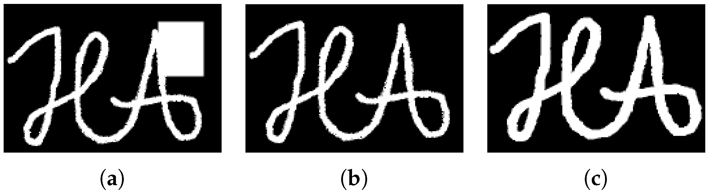
Figure 1 demonstrates the contradiction between the Hamming distance and subjective human judgments. However, every human observer would judge the middle-right pair to be more similar; the Hamming distances between the middle and left and the distance between the middle and right images are exactly the same. Our perception is based not only on the area of the differing parts, but also on shape-related information. This information cannot be ignored if we want to create a trustworthy metric. One can see that the Hamming distance (and any other area-based metric) can provide misleading decisions. Thus, shape-related descriptors are also required.
The other often used metric is the Hausdorff distance [16], which is determined solely by the distance of the furthest different pixel between the objects:
where , d is a distance measure (e.g., or ), F and G are the images to be compared and f and g represent their pixels. This distance represents topology better since Hamming distance is determined only by the area of the different pixels; meanwhile, here it ensures that all differences are in a radius. Since this metric can reflect topology better, it is employed in certain applications such as geology [20] and quantum physics [21]. Unfortunately, this metric’s sensitivity to noise prevents its utilization in practical applications. If the largest distances between two different pixels are the same on two image pairs, the metric will return the same result and hides all other information about shapes as well.
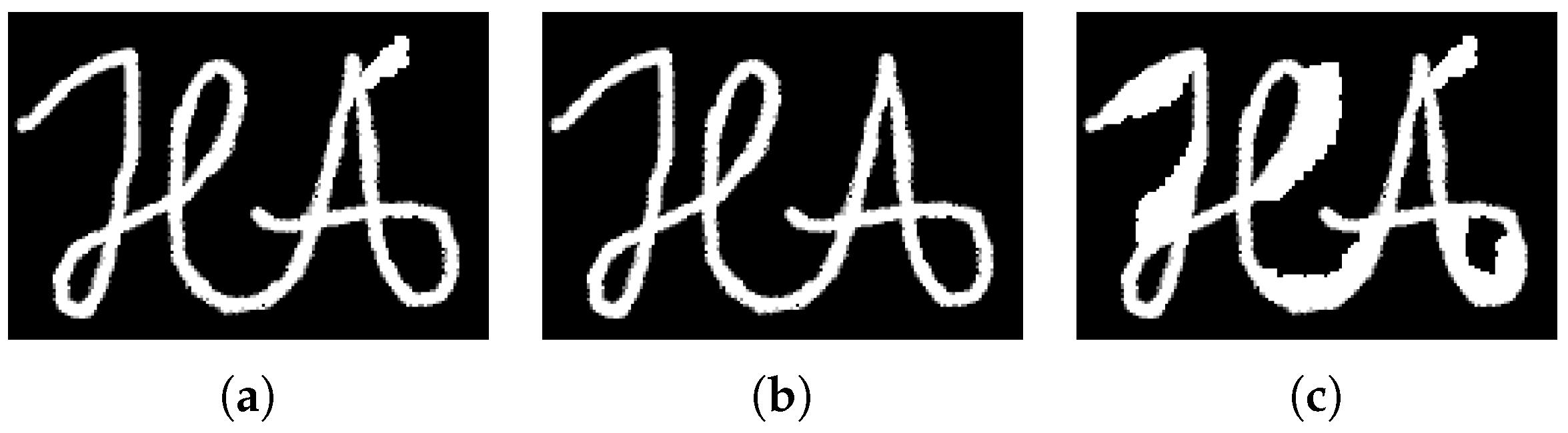
The illustration of the Hausdorff distance and its poor applicability can be seen in Figure 2. This image illustrates the contradiction between the Hausdorff distance and subjective judgments. Hausdorff distances between the image in the middle and the one to the left and between the image in the middle and the one to the right are exactly the same. A human observer would most probably select the middle-left pair as more similar images. Natural vision and perception is not only based on the topology of the differing parts, but also on area-based information. This information also has to be considered during computation to produce a reliable and useful metric.
Binary Wave Metric
Both the Hamming and Hausdorff metrics reveal important properties about similarity, but to create a multipurpose, efficient metric, their advantageous properties should be combined, eliminating their flaws. The application of different metrics in a parallel manner might be beneficial, but in the case of simultaneously computed metrics one will increase processing time and algorithmic complexity and we may not be able to solve the problem since the weighting of these metrics during combination is always problematic. One has eventually to combine all the metrics into a single function that results in a scalar to ease classification and comparison.
The idea of the binary wave metric was first introduced by Istvan Szatmari in 1999 [22]. His work covers the metric calculation for convex, binary objects only and in this work we will extend it to non-convex, grayscale images, which makes it applicable as a loss function in image segmentation algorithms. This metric can be defined as the volume of an ascending wave starting from the intersection of the objects and filling out the area defined by the union of the two binary objects.
On a suitable hardware architecture, the non-linear wave metric can measure both the shape and the area difference between two objects in a single operation (e.g., on a multi-layer cellular neural network) [23].
Based on this, the equation of the metric calculation for convex two-dimensional binary objects can be given as the following:
which is the point-wise integration of local Hausdorff distances over every point in the disjunctive union of the two objects. In the case of non-convex objects, the non-linear wave metric is the integration of the local Hausdorff distances along the shortest path in the union of the two sets.
It can be easily seen that the wave metric contains and compresses both previously introduced metrics. The maximal height of the ascending wave (the propagation time of the wave) is proportional to the value of the Hausdorff metric () for connected objects and the area of the wave propagation is proportional to the Hamming distance ().
The slope, the increase of the wave for each step, determines the connection between the topological (Hausdorff) and the area-based (Hamming) information. For example, if this increase is set to zero and propagation starts with a constant non-zero magnitude, the wave metric will yield the Hamming distance multiplied by the initial constant. In the case of a larger slope, the metric will shift more towards the Hausdorff metric and the distances between the further and further differing points will determine the result more and more.
It is easy to see that this similarity function fulfills almost all the required properties of a metric. It can be defined as a function on a given set and it fulfills the following properties (): non-negativiy or separation axiom: ; identity of indiscernibles, or coincidence axiom: ; and symmetry: .
Unfortunately, the triangle inequality or subadditivity axiom
does not hold this way since three objects, from which two are completely disjoint (a and c) and the third of which has a common part with both (b), would result in a zero value for and a non-zero value for both and . To get around this problem, we applied an extra penalty for points which cannot be reached in the union during wave propagation. This penalty has to be larger than the maximum penalty in the reachable region. With this addition, the wave metric fulfills all the axioms and forms a proper metric for non-connected objects as well.
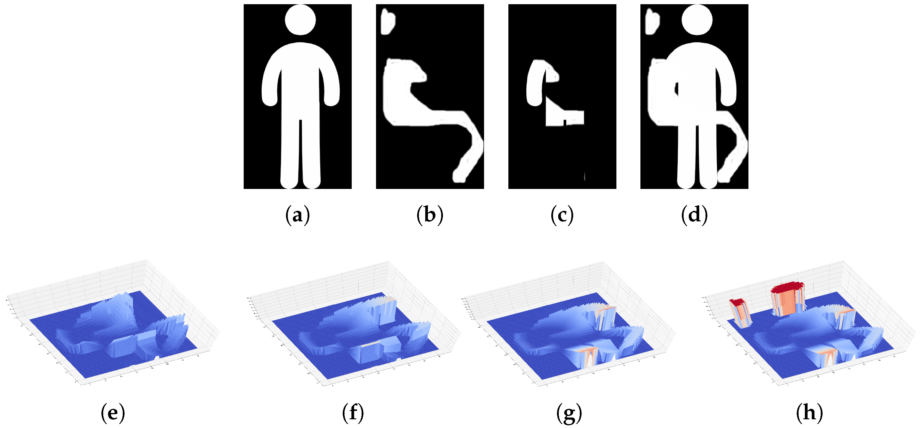
The illustration of the wave propagation and the metric can be seen in Figure 3. In this image, the first row depicts two possible binary input images (first and second images from the left) and their intersection and union (third and fourth images from the left). The last two rows depict four 3D versions of the wave metric in an increasing manner until reaching the union at iterations 100, 150, 300 and the last iteration, including not reached regions. During propagation, further and further pixels will be incorporated in the loss function with higher and higher values. At the last step, a high penalty will be assigned to all pixel which were not reached during propagation.
This metric can be used to compare images and accurate usable calculations, but unfortunately cannot be used during network training, as was shown in [24], since it can only be calculated between two binary images.
3. Wave Loss: Extension of the Wave Metric to Three Dimensions
In the previous section, the binary wave metric was described; as was demonstrated, it creates a connection between topological and area-based metrics. To extend it to grayscale images and two-dimensional probability distributions, we have to consider intensity-based differences as well. The metric should depend on three not-independent measures: the area of the differences, the topology of the differences and the intensities and values of the differences.
In this case the output and ground-truth images can be imagined as two two-dimensional surfaces in three dimensions. From this, we can calculate the intersection and the union (which will also be two-dimensional surfaces); then, the metric can be imagined as a three-dimensional wave propagating and filling out the space between these two surfaces. A weight will be associated to every new voxel at each time step of the propagation and this four-dimensional volume (the weighted sum of the three-dimensional changes) will be called wave loss.
Our goal was to differentiate between value and topology-based differences and because of this the propagation speed of the wave is different in z (intensity) and x, y (topological directions) (the wave could propagate differently along the x and y dimensions as well, but in image-processing applications these dimensions are usually handled in the same manner).
Compared to the binary wave metric, where only topological distances were covered, an upper bound for the number of required steps until convergence can easily be identified. An upper bound for spatial propagation can also be found (identifying the object containing the longest possible path with the given image size), but this bound is fairly high compared to the number of steps required to cover differences in intensity. In practice, this means that typically a small number of iterations (10–20) is enough to calculate the metric.
Algorithm 1 calculates wave loss for two grayscale images. The input values are and and the output of the algorithm is a scalar variable . The parameters of the algorithm are the following:
- will determine how fast the wave propagates along the intensity differences; every pixel’s intensity will be increased by this amount in every iteration. This parameter will also determine the maximum number of required iterations and by this it will also determine the largest distance from the intersection where topological differences are considered. Having a larger distance than the maximal receptive field of a neuron in the network is illogical because this way the error could be derived back to a neuron which had no vote in the classification of that input pixel. In our experiments, this value was between 0.05 and 0.1, meaning that the wave from a selected point could propagate for 20 and 10 pixels.
- will determine the spatial propagation speed of the wave. Spatial propagation is implemented by a max pooling operation with window size and a stride of one. In our simulations, this value was always set to 3.
- is a vector of penalties for the intensity differences. If this value is constant, the weight differences will be linearly proportional to the penalties in the loss. If this is increasing, it means larger differences (where more iterations are required to reach the desired value) will have larger and larger penalties. In our simulations, we used constant values in .
- is a vector containing the penalties for topographical differences. will weight those points which can be reached in one spatial propagation and which are in the direct neighborhood of the intersection. will have a penalty for those values which will be reached at the k-th iteration. In our simulations, we applied linearly increasing values which were all lower than the values of . In most networks, we want to have good results on average, but minor mistakes about the shape of the object can be tolerated. Applying lower values than the intensity weights () means that the importance of the shape of the segmented object will become less important. Monotonically increasing means that the further we are from the object, the higher the cost a misclassification will result. Applying higher weights than , which are monotonically decreasing, would mean that the boundaries are really important and classifying a pixel around a boundary is a larger problem than misclassifying a pixel somewhere far from the object.
| Algorithm 1: Calculation of wave loss. |
 |
Since both the values in and are bounded, the algorithm will always converge if a larger than zero parameter is applied. The difference between the intersection and the union will decrease at least by amount in every iteration. Since both the intersection and the union are probability distributions in the case of neural network training (just like and ) we can consider their values to be between zero and one and this way the algorithm will always converge in iterations. One can easily see that the wave metric is an extension of the normal metric; if there is no spatial propagation () and ValW values are all the same, we will obtain L1 loss as a result.Similarly, if the values in ValW are increasing exponentially with no spatial propagation, this metric will calculate the traditional cross entropy between the two images, representing two-dimensional distributions.
The derivative of Algorithm 1 is also required for network training. Luckily, our method consists of simple operations such as addition, multiplication and maximum/minimum selection. The derivative of all of these individual operations (each line in the algorithm) can be calculated in a straightforward manner and the derivative of the algorithm can be determined by the chain rule. Luckily, in modern machine-learning frameworks such as Pytroch [25] or Tensorflow [26] where automatic differentiation is applied, these derivatives are calculated automatically.
During the calculations, we first increase according to the intensities. This is a global change and it happens everywhere in the image where the values have not reached the union and after this step we apply spatial propagation. One could change this order, but we considered intensity-based differences more important. One could also execute both propagations separately and sum their penalties, but we did not observe any measurable effect applying this modification. In this setup, compared to the binary implementation all points are reached during propagation since the intensity differences are limited; therefore, there is no need for an extra penalty for unreached regions.
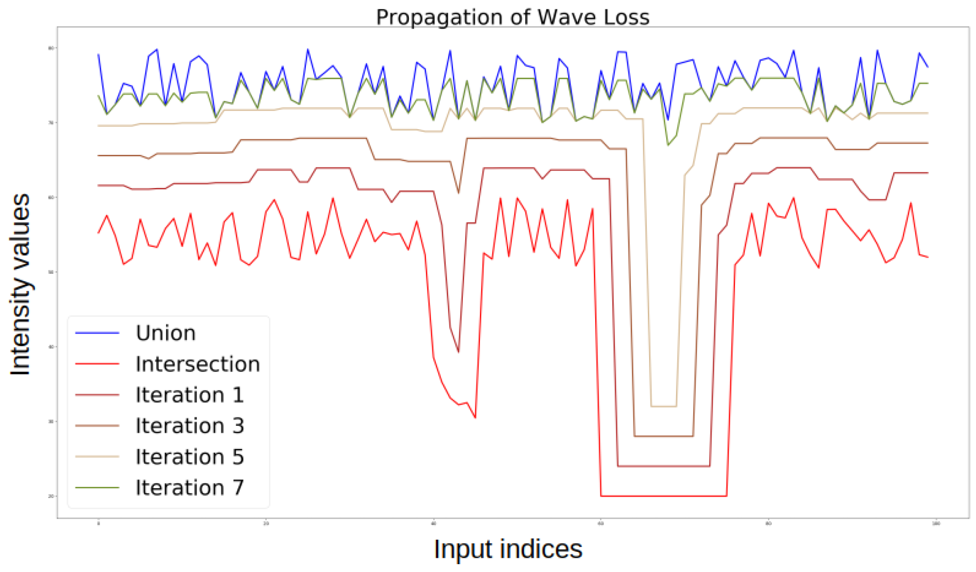
Since it is difficult to plot wave loss using two-dimensional images, we opted to display it using two one-dimensional grayscale ‘images’. This can be seen in Figure 4. As can be seen, the wave fills out the region between the intersection and the union of the two surfaces. At each propagation, the newly reached pixels will be weighted and added to the loss function. This way, this metric incorporates intensity-, area- and shape-related information simultaneously.
From an implementation point of view, value increase is just an addition and spatial propagation is a grayscale dilation, which is essentially a max pooling operation which can be found in every modern machine-learning environment. For a training step, the number of additional pooling operations is fairly small compared to the pooling operations already contained by a typical convolutional neural network. Therefore, the calculation of the wave loss will not increase training time significantly and has no effect on inference time.
4. Materials and Methods
We used the Pytroch [25] open source machine-learning framework for the implementation of our algorithm and for training various neural network architectures on multiple datasets. For evaluation, we investigated three publicly available and commonly cited datasets: CLEVR [27], Cityscapes [28] and MS-COCO [14]. In our instance segmentation experiments on MS-COCO, we used the Detectron 2 environment [29]. For the sake of reproducibility and a detailed description of parameter setting, our code for network training and evaluation on both datasets along with the data generation script for the CLEVR dataset can be found at https://github.com/horan85/waveloss (accessed on 28 May 2022).
4.1. Simple Dataset for Segmentation
Since we were not able to find a simple segmentation dataset (like MNIST [30] or CIFAR for classification), we created a simple dataset based on CLEVR [27].
The dataset contains 25,200 three-channel RGB images (of size ) of simple objects along with their instance masks, amodal masks and pairwise occlusions and three-dimensional coordinates for each object. These images were created in a simulated environment and contain cylinders, spheres and cubes in various positions. Since the dataset is simulated, the exact location and the pixel-based segmentation maps of all the images are known. This results in a simple dataset for various tasks, like three-dimensional reconstruction, instance segmentation and amodal segmentation.
The dataset contains objects of simple shapes, but also contains shadows, reflections and different illuminations, which make it relevant for the evaluation of segmentation algorithms.
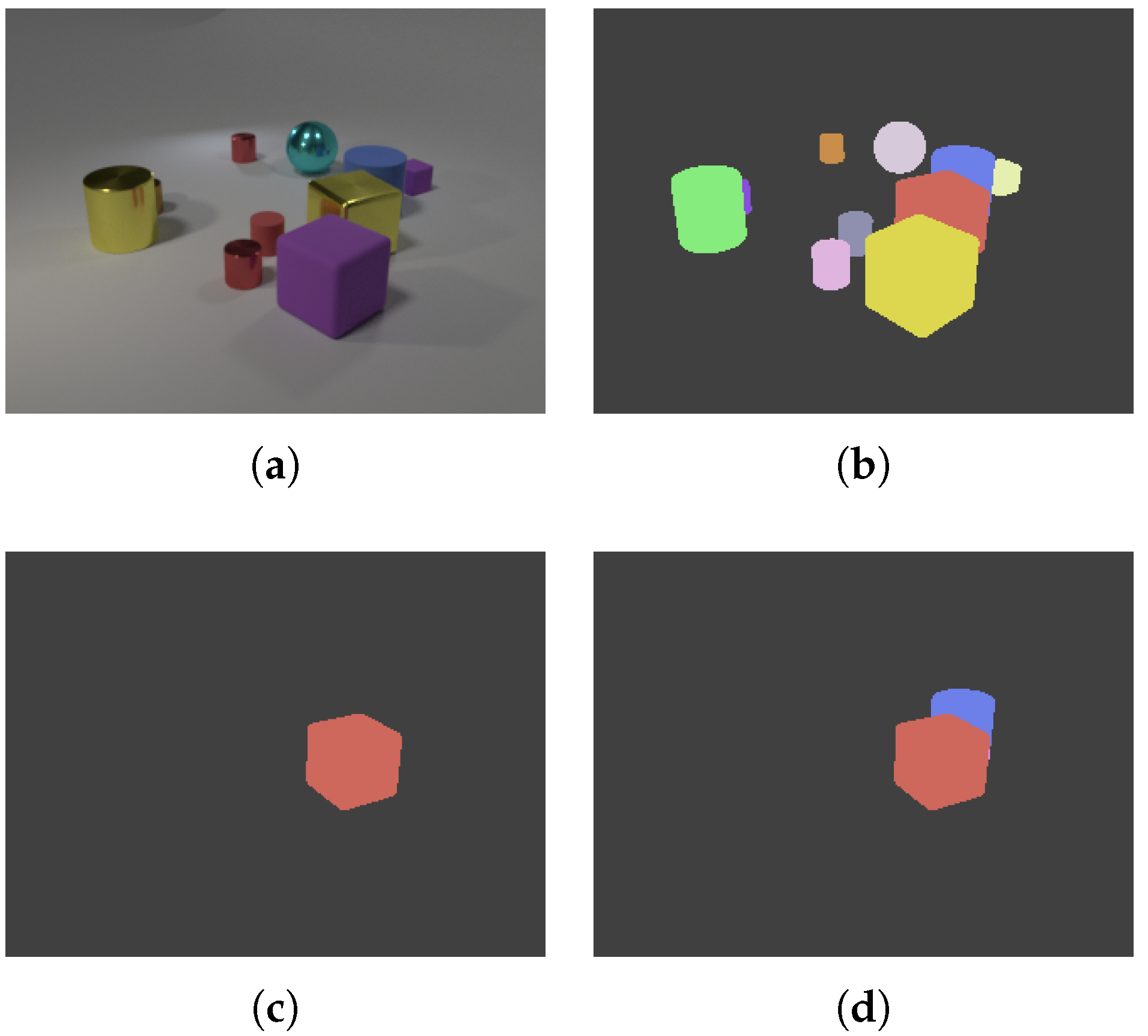
An example image of the dataset along with a few generated masks can be seen in Figure 5. An input image (top left), the instance segmentation mask (top right), an example amodal mask which was generated for each object individually (bottom left) and the pairwise occlusion mask (bottom right) are displayed in this figure. The pairwise occlusion images with the amodal mask can be used to determine front–back relation between objects. Apart from the mask, the exact object coordinates and sizes are also stored in JSON format.
A simple simulated dataset: CLEVR
We selected the U-net architecture to compare wave loss and L1 loss in our simple CLEVR-inspired dataset. We used a U-NET-like structure containing 8, 16, 32, 64 convolution blocks (each ). Downscaling was carried out by strided convolutions, while upscaling was implemented by transposed convolutions.
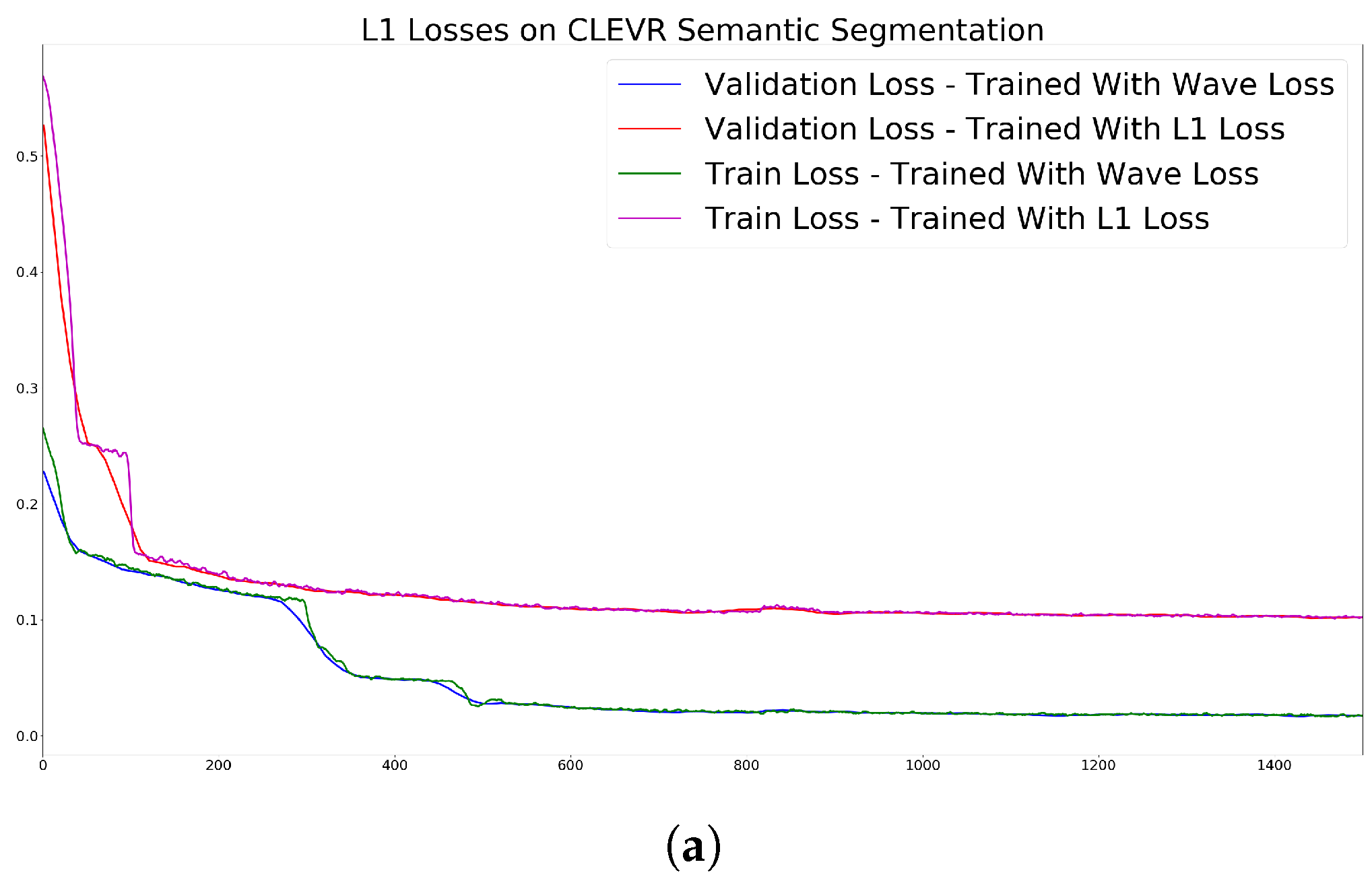
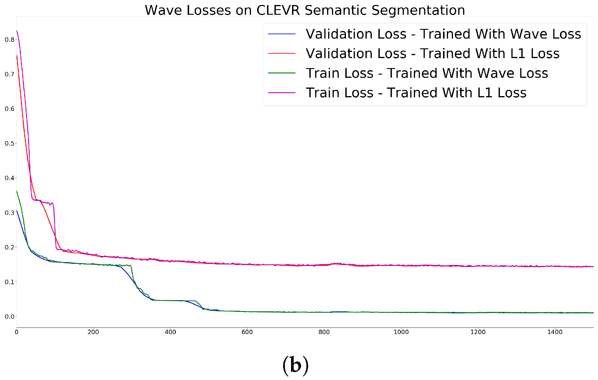
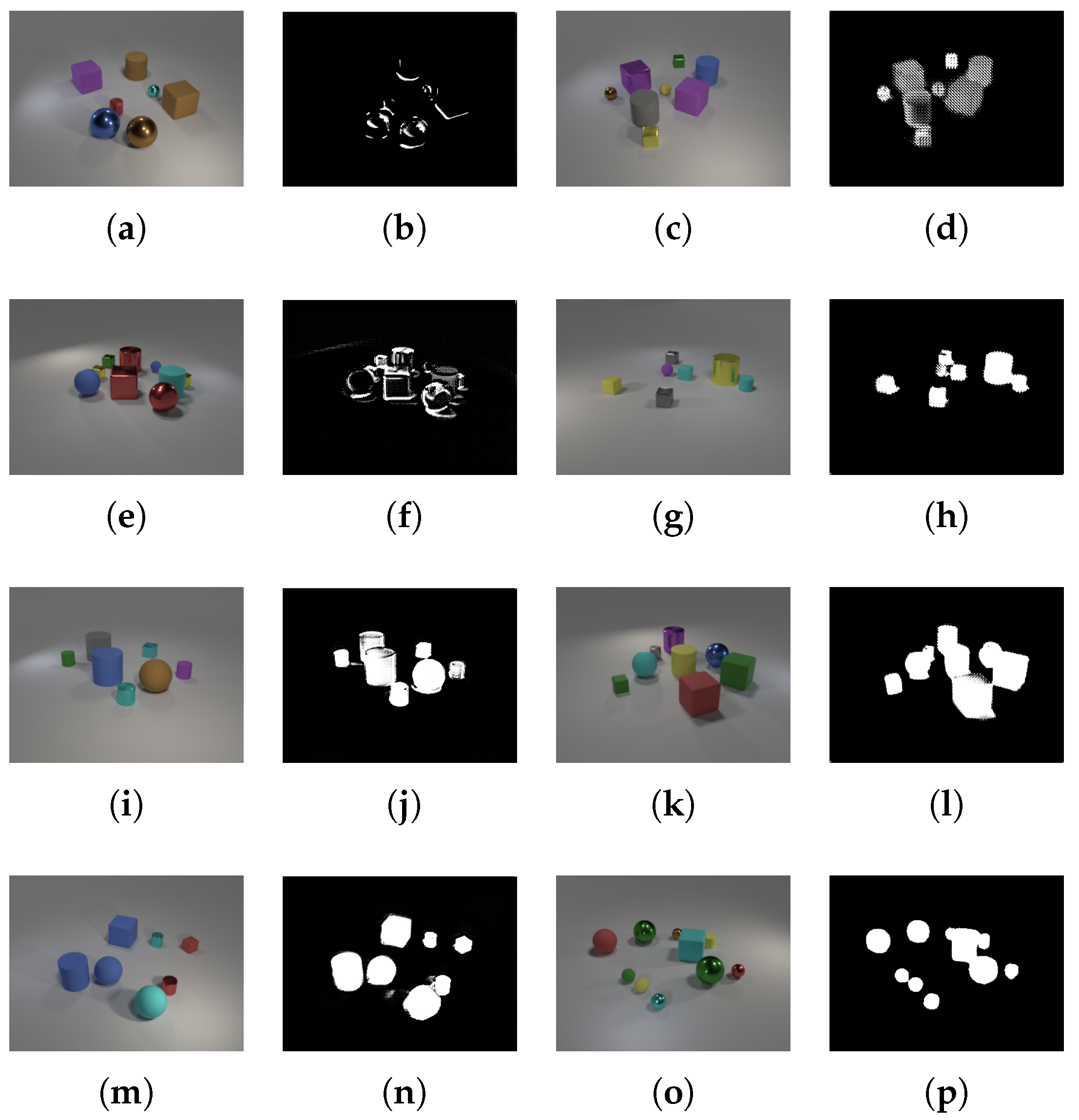
We trained the network 20 times independently on our dataset for semantic segmentation, using 23,400 images for training and 1800 images for validation (all the validation scenes were generated independently from the training scenes). In one setup, we trained the network to minimize the L1 loss on the training set, in the other setup wave loss was defined as the error function. In both cases, we measured both L1 and wave loss during training and validation. The losses can be seen in Figure 6. Some qualitative examples from the validation set during different train iterations can be seen in Figure 7. The images were taken at 200, 400, 600, 1000 iterations from the training set. From left to right, the columns are the following: input image, network output trained with L1 loss, input image, network output trained with wave loss. One could also observe a formation of a spotted, grid-like structure at the first iterations of training using the wave loss since regions around high intensity pixels cause lower loss values.
As one can see from these measurements, wave loss results in faster convergence and better accuracy in both the training and the validation sets.
These simple examples show the applicability of wave loss in segmentation tasks, but to demonstrate the advantage of this topological loss function, we have to investigate it in more complex and practical tasks.
5. Results
Semantic segmentation on Cityscapes
We investigated the Cityscapes dataset [28] with the following architectures: SegNet [3], HRNET [31], DeepLab [32] and DeepLabv3 [33].
We trained these networks with three different loss functions (, cross entropy and wave loss) and the accuracy results can be found in Table 1.
During training, we initialized the weights randomly and executed five independent trainings with every configuration and trained them for 400,000 iterations.
The parameters of our loss function were the following: SpaInc was set to three; this means propagation happened using kernels. Topology weights (SpaW) exponentially increased from 0.01 to 1 and intensity weights (ValW) were all set to a constant value of one. ValInc was set to 0.05; this means that the largest value gap of one will be filled in twenty iterations. Using this value, neighborhoods of maximum twenty pixels are affected by wave propagation. Since the input resolution of the networks was , we considered these neighbourhoods sufficiently large.
As can be seen from the results, the application of wave loss increased the network performance compared to traditionally used cross entropy loss with an approximated 3% in the case of all network architectures and provided better segmentation accuracy than any of the investigated loss functions in all cases.
Instance segmentation on MS-COCO
We also investigated the problem of instance segmentation on COCO 2017 [14]. We investigated MASK-RCNN with different backbone architectures using the Detectron 2 framework where we kept the architecture and all the other parameters unchanged in the configuration files used for instance segmentation on this dataset. These configurations contained data augmentation in the input samples containing random flip, random crop, brightness change and random additive noise. The original training script used cross entropy and we added our implementation of the wave loss to the framework and compared its performance.
The parameters of our loss function were the same as in the case of the Cityscapes dataset. We would like to emphasize that the images used for segmentation differ significantly in size from the images used in Cityscapes since in the case of Mask R-CNN the segmentation head is executed on the outputs of the RoiAlign layer. Even though the object sizes may differ, the same parametrization worked well for this architecture and dataset as well, which demonstrate that our loss function is not heavily dependent on the exact parameter values.
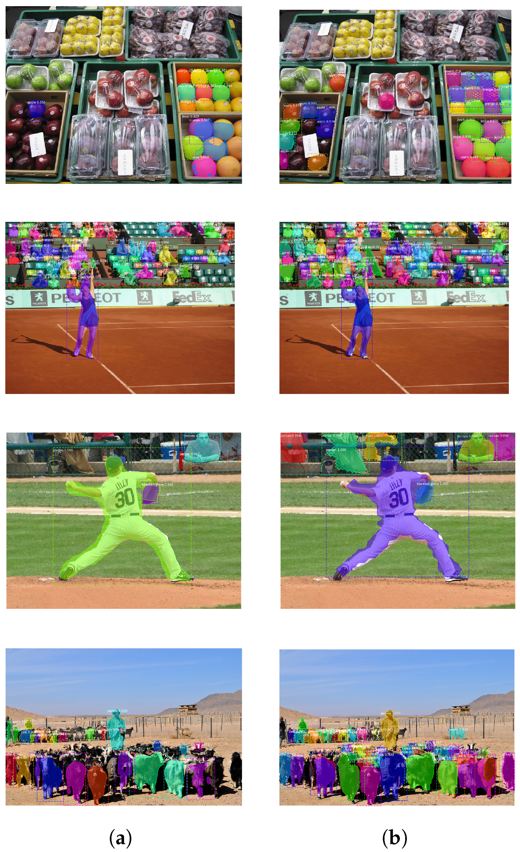
We measured mean average precision values using the evaluation script of COCO. We have to note that IOU is more related to wave loss than to L1 metric or cross entropy since wave loss uses the intersection and union to determine wave propagation, but we think this does not bring an unfair bias to the evaluation. The results can be seen in Table 2. As can be seen from the results, the application of the wave loss increased the precision of the network with an overall on our validation set and the network performs especially better in the case of small objects, where an improvement of was achieved compared to our reference network trained by cross entropy loss. We also have to emphasize that segmentation improved in the case of every architecture and for all object sizes. Qualitative results about the generated masks and bounding boxes can be seen in Figure 8. The segmentation masks in the first column were generated by a network trained with cross entropy loss; the masks in the second column are results of a network trained with wave loss. As can be seen, wave loss does not cover boundaries as sharply, but altogether gives a better coverage of the objects. (Although we have to note that this judgment might be subjective and could also depend on the exact parmetrization of wave loss).
6. Discussions
Our results presented in the previous section clearly demonstrate that incorporating topological information in the loss function can improve the segmentation accuracy of various network architectures. The results in Table 1 and Table 2 demonstrate that our approach not only improved the accuracy by on average but also performs better than any of the other loss functions selected for comparison.
We have compared our method to a recent reformulation of Dice loss [17], which calculates the ratio between the intersection and the union between the two binary objects. Unfortunately, Dice loss is a metric applied over binary images and they are based solely on area-based differences. Until the number of pixels in the intersection and union remain the same, the regions can change arbitrarily. Namely, the different pixels can move anywhere in the image space; only the number of different pixels matters. Another recent improvement over the area-based metric is the active boundary loss [34] where, as an additional loss value, the boundary pixels are calculated with a larger weight, this way representing the shape of the object in the loss function. This is more similar to our approach, but it considers only the boundary pixels and no other pixels in the differing area. The third selected loss is the shape aware loss function [35] which considers all pixels in a differing region, but with a precomputed weight which is the pixels’ Euclidean distance from the intersection. Unfortunately, this distance is not the same as the shortest path of differing pixels since in the case of non-convex regions this distance can be significantly larger. One can easily see that incorporating more topographic information in the loss functions improved segmentation accuracy and the best results could be achieved with wave loss. We also have to note that our method is not another completely different loss function, but a combination and generalization of area- and distance-based metrics. For example, setting the parameter to an all zero vector except the first value will result in the spatial information being incorporated only at one pixel from the intersection, which is exactly the same region as the boundary of the object. This way, one can calculate boundary loss using our method. Similarly, if all values are zero our metric will compute an area-based metric, similar to the Hamming distance or Dice score. On the other hand, if parameters are all set to zero, only the distance of the differing pixels will be a determining factor similarly to Hausdorff distance. These results show that our approach defines a more general metric which can mimic most of the previously applied loss functions and with proper parameterization it can also perform better in practical applications.
7. Conclusions
In this paper, we have shown how a topographic metric can help in the increase of the accuracy of commonly applied image segmentation networks during training, and results in higher accuracy and precision in evaluation. We have shown on a simple dataset, inspired by CLEVR, that the same network can achieve better accuracy and faster convergence using wave loss rather than pixel-based loss functions.
We have also shown, in more complex tasks, that the overall accuracy of instance segmentation could be increased by on MS-COCO using the Mask R-CNN architecture, with a ResNet-101 backbone, modifying only the loss function from cross entropy to wave loss.
We have also demonstrated on the Cityscapes dataset that the inclusion of topographic information in the loss function can increase the test accuracy by on average compared to cross entropy, which was observed in the case of four different architectures (SegNet, DeepLab, DeepLabV3 and HRNet). We also compared wave loss to other recently published loss functions such as Dice loss, active boundary loss and shape aware loss and our approach provided higher segmentation accuracy in all cases.
These results are initial and further detailed investigations are needed using various networks, datasets and parameter settings, but we believe they are promising and demonstrate that including topographic information in loss calculation can result in higher IOU measures in all segmentation problems.
Author Contributions
All authors have contributed equally to this research. All authors have read and agreed to the published version of the manuscript.
Funding
This research received funding from grants 2018-1.2.1-NKP-00008: Exploring the Mathematical Foundations of Artificial Intelligence TKP2021_02-NVA-27—Thematic Excellence Program.
Institutional Review Board Statement
Not applicable.
Informed Consent Statement
Not applicable.
Data Availability Statement
Our methods were evaluated on public datasets except our results in Section 4.1 for which the data generation script can be found at https://github.com/horan85/waveloss (accessed on 28 May 2022).
Conflicts of Interest
The authors declare no conflict of interest.
References
- Ronneberger, O.; Fischer, P.; Brox, T. U-net: Convolutional networks for biomedical image segmentation. In Proceedings of the International Conference on Medical Image Computing and Computer-Assisted Intervention, Munich, Germany, 5–9 October 2015; pp. 234–241. [Google Scholar]
- Ros, G.; Sellart, L.; Materzynska, J.; Vazquez, D.; Lopez, A.M. The synthia dataset: A large collection of synthetic images for semantic segmentation of urban scenes. In Proceedings of the IEEE Conference on Computer Vision and Pattern Recognition, Las Vegas, NV, USA, 27–30 June 2016; pp. 3234–3243. [Google Scholar]
- Badrinarayanan, V.; Kendall, A.; Cipolla, R. Segnet: A deep convolutional encoder-decoder architecture for image segmentation. IEEE Trans. Pattern Anal. Mach. Intell. 2017, 39, 2481–2495. [Google Scholar] [CrossRef] [PubMed]
- He, K.; Gkioxari, G.; Dollár, P.; Girshick, R. Mask r-cnn. In Proceedings of the IEEE International Conference on Computer Vision, Venice, Italy, 22–29 October 2017; pp. 2980–2988. [Google Scholar]
- Lin, T.Y.; Goyal, P.; Girshick, R.; He, K.; Dollár, P. Focal loss for dense object detection. IEEE Trans. Pattern Anal. Mach. Intell. 2018, 2980–2988. [Google Scholar]
- Long, J.; Shelhamer, E.; Darrell, T. Fully convolutional networks for semantic segmentation. In Proceedings of the IEEE Conference on Computer Vision and Pattern Recognition, Boston, MA, USA, 7–12 June 2015; pp. 3431–3440. [Google Scholar]
- Gupta, S.; Girshick, R.; Arbeláez, P.; Malik, J. Learning rich features from RGB-D images for object detection and segmentation. In Proceedings of the European Conference on Computer Vision, Zurich, Switzerland, 6–12 September 2014; pp. 345–360. [Google Scholar]
- Zhu, Y.; Tian, Y.; Metaxas, D.N.; Dollár, P. Semantic Amodal Segmentation. In Proceedings of the IEEE Conference on Computer Vision and Pattern Recognition, Honolulu, HI, USA, 21–26 July 2017; Volume 2, p. 7. [Google Scholar]
- Schmidt, M.; Fung, G.; Rosales, R. Fast optimization methods for l1 regularization: A comparative study and two new approaches. In Proceedings of the European Conference on Machine Learning, Warsaw, Poland, 17–21 September 2007; pp. 286–297. [Google Scholar]
- Hu, X.; Li, F.; Samaras, D.; Chen, C. Topology-preserving deep image segmentation. Adv. Neural Inf. Process. Syst. 2019, 508, 5657–5668. [Google Scholar]
- Clough, J.; Byrne, N.; Oksuz, I.; Zimmer, V.A.; Schnabel, J.A.; King, A. A topological loss function for deep-learning based image segmentation using persistent homology. arXiv 2019, arXiv:1910.01877. [Google Scholar] [CrossRef] [PubMed]
- Shit, S.; Paetzold, J.C.; Sekuboyina, A.; Ezhov, I.; Unger, A.; Zhylka, A.; Pluim, J.P.; Bauer, U.; Menze, B.H. clDice-a Novel Topology-Preserving Loss Function for Tubular Structure Segmentation. In Proceedings of the IEEE/CVF Conference on Computer Vision and Pattern Recognition, Virtual, 19–25 June 2021; pp. 16560–16569. [Google Scholar]
- Kervadec, H.; Bouchtiba, J.; Desrosiers, C.; Granger, E.; Dolz, J.; Ayed, I.B. Boundary loss for highly unbalanced segmentation. In Proceedings of the International Conference on Medical Imaging with Deep Learning, London, UK, 8–10 July 2019; pp. 285–296. [Google Scholar]
- yi Lin, T.; Maire, M.; Belongie, S.; Hays, J.; Perona, P.; Ramanan, D.; Zitnick, C.L. Microsoft COCO: Common Objects in Context; Springer: Cham, Switzerland, 2014. [Google Scholar]
- Hamming, R.W. Error detecting and error correcting codes. Bell Syst. Tech. J. 1950, 29, 147–160. [Google Scholar] [CrossRef]
- Henrikson, J. Completeness and total boundedness of the Hausdorff metric. MIT Undergrad. J. Math. 1999, 1, 69–80. [Google Scholar]
- Zhao, R.; Qian, B.; Zhang, X.; Li, Y.; Wei, R.; Liu, Y.; Pan, Y. Rethinking dice loss for medical image segmentation. In Proceedings of the 2020 IEEE International Conference on Data Mining (ICDM), Sorrento, Italy, 17–20 November2020; pp. 851–860. [Google Scholar]
- Berman, M.; Triki, A.R.; Blaschko, M.B. The lovász-softmax loss: A tractable surrogate for the optimization of the intersection-over-union measure in neural networks. In Proceedings of the IEEE Conference on Computer Vision and Pattern Recognition, Salt Lake City, UT, USA, 18–23 June 2018; pp. 4413–4421. [Google Scholar]
- Abraham, N.; Khan, N.M. A novel focal tversky loss function with improved attention u-net for lesion segmentation. In Proceedings of the 2019 IEEE 16th International Symposium on Biomedical Imaging (ISBI 2019), Venice, Italy, 8–11 April 2019; pp. 683–687. [Google Scholar]
- Outcalt, S.I.; Melton, M.A. Geomorphic application of the hausdorff-besicovich dimension. Earth Surf. Process. Landf. 1992, 17, 775–787. [Google Scholar] [CrossRef]
- Latrémolière, F. Quantum metric spaces and the Gromov–Hausdorff propinquity. Noncommut. Geom. Optim. Transp. Contemp. Math 2016, 676, 47–133. [Google Scholar]
- Szatmári, I.; Rekeczky, C.; Roska, T. A nonlinear wave metric and its CNN implementation for object classification. J. VLSI Signal Process. Syst. Signal Image Video Technol. 1999, 23, 437–447. [Google Scholar] [CrossRef]
- Roska, T.; Chua, L.O. The CNN universal machine: An analogic array computer. IEEE Trans. Circuits Syst. Ii Analog. Digit. Signal Process. 1993, 40, 163–173. [Google Scholar] [CrossRef]
- Al-Afandi, J.; Horvath, A. Application of the Nonlinear Wave Metric for Image Segmentation in Neural Networks. In Proceedings of the CNNA 2018: The 16th International Workshop on Cellular Nanoscale Networks and their Applications, Budapest, Hungary, 28–30 August 2018; pp. 1–4. [Google Scholar]
- Paszke, A.; Gross, S.; Chintala, S.; Chanan, G.; Yang, E.; DeVito, Z.; Lin, Z.; Desmaison, A.; Antiga, L.; Lerer, A. Automatic Differentiation in Pytorch. 2017. Available online: https://openreview.net/pdf?id=BJJsrmfCZ (accessed on 28 May 2022).
- Abadi, M.; Barham, P.; Chen, J.; Chen, Z.; Davis, A.; Dean, J.; Devin, M.; Ghemawat, S.; Irving, G.; Isard, M.; et al. {TensorFlow}: A System for {Large-Scale} Machine Learning. In Proceedings of the 12th USENIX Symposium on Operating Systems Design and Implementation (OSDI 16), Savannah, GA, USA, 2–4 November 2016; pp. 265–283. [Google Scholar]
- Johnson, J.; Hariharan, B.; van der Maaten, L.; Fei-Fei, L.; Zitnick, C.L.; Girshick, R. CLEVR: A diagnostic dataset for compositional language and elementary visual reasoning. In Proceedings of the IEEE Conference on Computer Vision and Pattern Recognition, Honolulu, HI, USA, 21–26 July 2017; pp. 1988–1997. [Google Scholar]
- Cordts, M.; Omran, M.; Ramos, S.; Rehfeld, T.; Enzweiler, M.; Benenson, R.; Franke, U.; Roth, S.; Schiele, B. The cityscapes dataset for semantic urban scene understanding. In Proceedings of the IEEE Conference on Computer Vision and Pattern Recognition, Las Vegas, NV, USA, 27–30 June 2016; pp. 3213–3223. [Google Scholar]
- Wu, Y.; Kirillov, A.; Massa, F.; Lo, W.Y.; Girshick, R. Detectron2. 2019. Available online: https://github.com/facebookresearch/detectron2 (accessed on 28 May 2022).
- LeCun, Y. The MNIST database of Handwritten Digits. 1998. Available online: http://yann.lecun.com/exdb/mnist/ (accessed on 28 May 2022).
- Cheng, B.; Xiao, B.; Wang, J.; Shi, H.; Huang, T.S.; Zhang, L. Higherhrnet: Scale-aware representation learning for bottom-up human pose estimation. In Proceedings of the IEEE/CVF Conference on Computer Vision and Pattern Recognition, Seattle, WA, USA, 13–19 June 2020; pp. 5386–5395. [Google Scholar]
- Liang-Chieh, C.; Papandreou, G.; Kokkinos, I.; Murphy, K.; Yuille, A. Semantic Image Segmentation with Deep Convolutional Nets and Fully Connected CRFs. In Proceedings of the International Conference on Learning Representations, San Diego, CA, USA, 7–9 May 2015. [Google Scholar]
- Chen, L.C.; Papandreou, G.; Kokkinos, I.; Murphy, K.; Yuille, A.L. Deeplab: Semantic image segmentation with deep convolutional nets, atrous convolution, and fully connected crfs. IEEE Trans. Pattern Anal. Mach. Intell. 2017, 40, 834–848. [Google Scholar] [CrossRef] [Green Version]
- Wang, C.; Zhang, Y.; Cui, M.; Liu, J.; Ren, P.; Yang, Y.; Xie, X.; Hua, X.; Bao, H.; Xu, W. Active boundary loss for semantic segmentation. arXiv 2021, arXiv:2102.02696. [Google Scholar]
- Al Arif, S.; Knapp, K.; Slabaugh, G. Shape-aware deep convolutional neural network for vertebrae segmentation. In Proceedings of the International Workshop on Computational Methods and Clinical Applications in Musculoskeletal Imaging, Quebec City, QC, Canada, 10 September 2017; pp. 12–24. [Google Scholar]
Figure 1.
Two images and a reference image with the same Hamming distances but different topology; (a) compared image 1; (b) reference image; (c) compared image 2.
Figure 1.
Two images and a reference image with the same Hamming distances but different topology; (a) compared image 1; (b) reference image; (c) compared image 2.

Figure 2.
Three images with the same Hausdorff distances but different topology; (a) compared image 1; (b) reference image; (c) compared image 2.
Figure 2.
Three images with the same Hausdorff distances but different topology; (a) compared image 1; (b) reference image; (c) compared image 2.

Figure 3.
Illustration of the wave propagation; (a) input A; (b) input B; (c) intersection; (d) union; (e) wave 100 iterations; (f) wave 150 iterations; (g) wave 300 iterations; (h) wave unreached regions.
Figure 3.
Illustration of the wave propagation; (a) input A; (b) input B; (c) intersection; (d) union; (e) wave 100 iterations; (f) wave 150 iterations; (g) wave 300 iterations; (h) wave unreached regions.

Figure 4.
The propagation of the wave during the calculation of wave loss.

Figure 5.
Example images from the CLEVR dataset; (a) input Image; (b) segmentation mask; (c) instance mask; (d) occlusion mask.
Figure 5.
Example images from the CLEVR dataset; (a) input Image; (b) segmentation mask; (c) instance mask; (d) occlusion mask.

Figure 6.
Losses on the CLEVR dataset averaged out on 20 independent runs; (a) L1 loss; (b) wave loss.
Figure 6.
Losses on the CLEVR dataset averaged out on 20 independent runs; (a) L1 loss; (b) wave loss.


Figure 7.
Example images at different iterations from the CLEVR dataset; (a) input; (b) seg. 200; (c) input; (d) seg. 200; (e) input; (f) seg. 400; (g) input; (h) seg. 400; (i) input; (j) seg. 600; (k) input; (l) seg. 600; (m) input; (n) seg. 1000; (o) input; (p) seg. 1000.
Figure 7.
Example images at different iterations from the CLEVR dataset; (a) input; (b) seg. 200; (c) input; (d) seg. 200; (e) input; (f) seg. 400; (g) input; (h) seg. 400; (i) input; (j) seg. 600; (k) input; (l) seg. 600; (m) input; (n) seg. 1000; (o) input; (p) seg. 1000.

Figure 8.
Example results on the COCO dataset segmented with Mask-RCNN; (a) cross entropy loss; (b) wave loss.
Figure 8.
Example results on the COCO dataset segmented with Mask-RCNN; (a) cross entropy loss; (b) wave loss.


Table 1.
This table contains the average accuracy results of five independent runs on the Cityscapes dataset using four different network architectures (rows) and six different loss functions for semantic segmentation.
Table 1.
This table contains the average accuracy results of five independent runs on the Cityscapes dataset using four different network architectures (rows) and six different loss functions for semantic segmentation.
| Model | L1 Loss | CrossEnt | Dice | Boundary | ShapeAware | Wave |
|---|---|---|---|---|---|---|
| SegNet | 54.2% | 57.0% | 57.3% | 57.7 | 58.6% | 59.5% |
| DeepLab | 59.7% | 63.1% | 64.1% | 64.3% | 65.4% | 66.7% |
| DeepLabv3 | 77.6% | 81.3% | 81.4% | 81.5% | 81.7% | 82.2% |
| HRNET | 77.4% | 81.6% | 81.8% | 81.8% | 82.1% | 83.4% |
Table 2.
Average precision results on COCO 2017 validation set using the same network architectures with three different loss functions in different columns (, cross entropy, Dice loss, active boundary loss, shape aware loss and wave loss). Two different architectures (ResNet-50 and ResNet-101) can be found in the rows, with feature pyramid networks (FPNs) or when the activation of the fourth convolution layer (C4) was used for region proposals. The results display the mean average precision for all objects, except the last three rows, where the accuracy results for the best performing network are detailed for small-, medium- and large-sized objects as well.
| Model | L1 | CrossEnt | Dice | Boundary | Shape | Wave |
|---|---|---|---|---|---|---|
| R50-C4 mAP all | 28.75% | 32.2% | 32.83% | 32.9% | 34.721% | 35.93% |
| R50-FPN mAP all | 29.43% | 35.2% | 36.14% | 36.12% | 37.53% | 38.11% |
| R101-C4 mAP all | 30.17% | 36.7% | 37.2% | 37.4% | 38.86% | 38.23% |
| R101-FPN mAP all | 31.67% | 38.6% | 38.8% | 39.3% | 40.25% | 41.7% |
| R101-FPN mAP s | 14.25% | 17.37% | 18.18% | 18.35% | 19.33% | 22.24% |
| R101-FPN mAP m | 37.53% | 39.23% | 39.74% | 40.52% | 41.27% | 43.26% |
| R101-FPN mAP l | 50.14% | 51.64% | 51.83% | 52.17% | 52.22% | 53.27% |
Publisher’s Note: MDPI stays neutral with regard to jurisdictional claims in published maps and institutional affiliations. |
© 2022 by the authors. Licensee MDPI, Basel, Switzerland. This article is an open access article distributed under the terms and conditions of the Creative Commons Attribution (CC BY) license (https://creativecommons.org/licenses/by/4.0/).
Share and Cite
MDPI and ACS Style
Kovács, Á.; Al-Afandi, J.; Botos, C.; Horváth, A. Wave Loss: A Topographic Metric for Image Segmentation. Mathematics 2022, 10, 1932. https://0-doi-org.brum.beds.ac.uk/10.3390/math10111932
AMA Style
Kovács Á, Al-Afandi J, Botos C, Horváth A. Wave Loss: A Topographic Metric for Image Segmentation. Mathematics. 2022; 10(11):1932. https://0-doi-org.brum.beds.ac.uk/10.3390/math10111932
Chicago/Turabian StyleKovács, Ákos, Jalal Al-Afandi, Csaba Botos, and András Horváth. 2022. "Wave Loss: A Topographic Metric for Image Segmentation" Mathematics 10, no. 11: 1932. https://0-doi-org.brum.beds.ac.uk/10.3390/math10111932
Note that from the first issue of 2016, this journal uses article numbers instead of page numbers. See further details here.