Unsteady Separated Stagnation-Point Flow Past a Moving Plate with Suction Effect in Hybrid Nanofluid

Abstract

Previous research has shown that incorporating stagnation-point flow in diverse manufacturing industries is beneficial due to its importance in thermal potency. Consequently, this research investigates the thermophysical properties of the unsteady separated stagnation-point flow past a moving plate by utilising a dual-type nanoparticle, namely a hybrid nanofluid. The impact of suction imposition on the entire hydrodynamic flow and heat transfer as well as the growth of boundary layers was also taken into account. A new mathematical hybrid nanofluid model is developed, and similarity solutions are obtained in the form of ordinary differential equations (ODEs). The bvp4c approach in MATLAB determines the reduced ODEs estimated solutions. The results show that increasing the stagnation strength parameters expands the skin friction coefficient and heat transfer rate. The addition of the suction parameter also resulted in an augmentation of thermal conductivity. Interestingly, reducing the unsteadiness parameter proportionately promotes heat-transfer performance. This significant involvement is noticeable in advancing industrial development, specifically in the manufacturing industries and operations systems.

1. Introduction

The investigation of unsteady boundary layer flow is essential since most of the flow problems in applied fluid mechanics are practically unsteady. This type of flow dynamics is currently being explored to quantify the friction drag and gain a better understanding due to its universal applications in diverse fields of engineering and applied science. Over the last few decades, the scientific world has paid close attention to understanding the unsteady behaviour of boundary layer flows, including the separated stagnation-point flow under various conditions. According to Blasius [1] and Prandtl [2], a characteristic for separation is also a factor for disappearing skin friction in the case of steady boundary-layer flow over a flat plate. Meanwhile, Sears and Telionis [3,4] demonstrated that the point of disappearing skin friction might not correlate with the point of separation. They also reported that the correlation between separation characteristics for the unsteady flow over fixed walls could provide comprehensive insight. The unsteady separated stagnation-point flow problem has been extensively studied, including several papers by Lok and Pop [5], Dholey [6,7], and Renuka et al. [8].

The study of boundary layer flow is prominent within the stagnation region in the manufacturing industry, for example, polymer productivity and extrusion process, which requires continuous advancement to comply with the quality standard [9,10]. The classic stagnation-point flow was first addressed by Hiemenz [11] and Homann [12]. Wang [13] and Takhar et al. [14] studied the steady and unsteady flow towards the stagnation region in cylindrical form. Dholey [15] investigated the magnetic effect of unsteady separated stagnation-point flow in electrically conducting and viscous fluid. Jamaludin et al. [16] investigated the suction imposition and radiation impact in the stagnation region of cross fluid.

As a result of the increased demand for effective methods to enhance heating devices’ performance, nanofluids have become far more essential in the last decades. Choi [17] initially projected the nanoparticle dispersion concept in a base fluid. Suresh et al. [18] have presented a characterisation of Al₂O₃-Cu nanocomposite powder and water-based nanofluids. Today, heat-transfer devices are used in almost every market sector, including medical drug carriers, solar collectors, computer processors, aerospace technology, and heat exchangers (see Chamsa-ard et al. [19]). Sharma et al. [20] found the dual solutions towards the unsteady separated stagnation-flow employing the finite element analysis in a nanofluid. The analysis of the heat transfers in the unsteady separated stagnation region of copper-water nanofluid utilising the Tiwari-Das model was presented by Rosça et al. [21]. Oztop and Abu-Nada [22] found that the heat-transfer enhancement caused by nanofluids was discovered to be more prominent at low aspect ratios than at high aspect ratios. It is worth mentioning that many references on nanofluids can also be found in the books by Das et al. [23], Minkovicz et al. [24], Shenoy et al. [25], Nield and Bejan [26], and Merkin et al. [27]. Meanwhile, Buongiorno et al. [28], Manca et al. [29], Mahian et al. [30,31], Kasaeian [32], and Gupta et al. [33] reviewed the insight into nanofluids applications and challenges. From another point of view, several experimental studies relating to micro-nano fluidic systems using a different approach of analysis and theoretical modeling have been discussed by [34,35,36,37]. Such articles contain interesting results and discoveries in the context of real-world application problems.

Following that, hybrid nanofluid has been used to improve the thermal mechanism by dispersing multiple nanoparticles in a base fluid. Hybrid nanofluids are new nanofluids made up of microscopic nanoparticles. Hybrid nanofluids are found in various areas, including heat transfer, where they have been used in mechanical heat sinks, plate heat exchangers, and helical heat exchangers (see Xian et al. [38]). Meanwhile, Devi and Devi [39,40,41] demonstrated that when a magnetic parameter is present, the heat-transfer rate of hybrid nanofluid is more significant than that of nanofluid. Takabi and Salehi [42] studied the heat-transfer performance of a sinusoidal corrugated enclosure by employing a hybrid nanofluid. Ghalambaz et al. [43] considered the mixed convection and stability analysis of stagnation-point boundary layer flow and heat transfer of hybrid nanofluids over a vertical plate. The published paper by Waini et al. [44], Khashi’ie et al. [45], and Zainal et al. [46,47,48] presented a comprehensive study on boundary-layer analyses in hybrid nanofluid. We also mention the very good review papers on hybrid nanofluids by Babu et al. [49] and Huminic and Huminic [50].

A thorough examination of the above-mentioned research is only conceivable to a limited extent. To the best of our knowledge, no previous studies have looked into the boundary layer flow and heat transfer of unsteady separated stagnation-point flow in dual-type nanoparticles. Henceforth, motivated by the work of Dholey [7,51], the goal of this study is to broaden the research by employing the hybrid nanofluid flow and the suction effect in boundary layer flow as well as heat transfer. In such a case, this research would like to examine the effect of suction imposition on the entire hydrodynamic flow and heat transfer as well as the growth of boundary layers in the unsteady separated stagnation region in a hybrid nanofluid. A new mathematical hybrid nanofluid model was developed, and we used the bvp4c scheme in the MATLAB package to elucidate the stated problem. Comparative results were obtained for a specific case, disclosing a good correlation with the existing outcomes. As there are multiple solutions aroused, an analysis of solution stability is performed to demonstrate the physical interpretations of the generated results. This significant engagement is important and could assist in advancing industrial development, particularly in the operations and manufacturing industries, for example, the transpiration cooling of a re-entry vehicle.

2. Mathematical Formulation

The present paper deals with the two-dimensional unsteady separated stagnation-point flow past a moving plate, as shown in Figure 1. The outer inviscid velocity is given by $u_e\left(x,t\right)=\alpha s\left(t\right)x$ and $v_e\left(y,t\right)=-\alpha s\left(t\right)\left(y-{\gamma }_1\right)$, where $\alpha \left(>0\right)$ is the constant stagnation flow strength, $s\left(t\right)=1/\xi \left(t_0-t\right)$ is the strain rate temporal variation, and ${\gamma }_1$ is the boundary layer displacement thickness that arises inside the layer caused by the fluid viscosity effect. The Cartesian coordinates given by $\left(x,y\right)$ with $x-$ axis taken are along the plate, and $y-$ axis is measured normal to it, while the flow is in the region $y\ge 0$, where $t$ denotes time. The constant wall temperature is $T_w$, and $T_{\infty }$ is the ambient temperature. Next, the plate moves with a velocity $u_w\left(x,t\right)$ proportional to $\epsilon -$times of the outer potential flow velocity $u_e\left(x,t\right)$. Physically, $\epsilon$ is the moving parameter, which may either be positive or negative accordingly as the plate moves in the same or the opposite direction of the outer inviscid flow, while $\epsilon =0$ means that the plate is not moving. Now, the respective problems can be modelled by (see Dholey [7]; Sharma et al. [20]):

$$\frac{\partial u}{\partial x}+\frac{\partial v}{\partial y}=0,$$

(1)

$$\frac{\partial u}{\partial t}+u\frac{\partial u}{\partial x}+v\frac{\partial u}{\partial y}=-\frac{1}{{\rho }_{hnf}/{\rho }_f}\frac{\partial p}{\partial x}+\frac{{\mu }_{hnf}/{\mu }_f}{{\rho }_{hnf}/{\rho }_f}\left(\frac{{\partial }^{2}u}{\partial x^2}+\frac{{\partial }^{2}u}{\partial y^2}\right),$$

(2)

$$\frac{\partial v}{\partial t}+u\frac{\partial v}{\partial x}+v\frac{\partial v}{\partial y}=-\frac{1}{{\rho }_{hnf}/{\rho }_f}\frac{\partial p}{\partial y}+\frac{{\mu }_{hnf}/{\mu }_f}{{\rho }_{hnf}/{\rho }_f}\left(\frac{{\partial }^{2}v}{\partial x^2}+\frac{{\partial }^{2}v}{\partial y^2}\right),$$

(3)

$$u\frac{\partial T}{\partial x}+v\frac{\partial T}{\partial y}=\frac{1}{\mathrm{Pr}}\frac{k_{hnf}/k_f}{{\left(\rho C_p\right)}_{hnf}/{\left(\rho C_p\right)}_f}\left(\frac{{\partial }^{2}T}{\partial x^2}+\frac{{\partial }^{2}T}{\partial y^2}\right),$$

(4)

subject to

$$\begin{array}{l}u=\epsilon u_w\left(x,t\right), v=v_w\left(t\right), T=T_w \mathrm{at} y=0,\\ u\to u_e\left(x,t\right), v\to v_e\left(y,t\right), T\to T_{\infty } \mathrm{as} y\to \infty ,\end{array}$$

(5)

where $u$ and $v$ are the velocity components along the $x-$ and $y-$axes, respectively; $v_w(t)$ is the velocity of wall mass transfer, where $v_w(t)>0$ and $v_w(t)<0$ signify as injection and suction procedure, respectively; and $\mathrm{Pr}={\left(\rho C_p\right)}_f/k_f$ is the Prandtl number. Further, note that ${\mu }_{hnf}$ is the dynamic viscosity, $k_{hnf}$ is the heat/thermal conductivity, and ${\rho }_{hnf}$ and ${\left(\rho C_p\right)}_{hnf}$ are the density and heat capacity, respectively.

Table 1. The characteristic properties (see Devi and Devi [39,40]).

Characteristics	Al2O3–Cu/H2O
Density	${\rho }_{hnf}=\left(1-{\varphi }_{hnf}\right){\rho }_f+{\varphi }_1{\rho }_{s1}+{\varphi }_2{\rho }_{s2}$
Dynamic viscosity	${\mu }_{hnf}=\frac{{\mu }_f}{{\left(1-{\varphi }_{hnf}\right)}^{2.5}}$
Thermal capacity	${\left(\rho C_p\right)}_{hnf}=\left(1-{\varphi }_{hnf}\right){\left(\rho C_p\right)}_f+{\varphi }_1{\left(\rho C_p\right)}_{s1}+{\varphi }_2{\left(\rho C_p\right)}_{s2}$
Thermal conductivity	$\frac{k_{hnf}}{k_f}=\left[\frac{\left(\frac{{\varphi }_1{k}_{s1}+{\varphi }_2{k}_{s2}}{{\varphi }_{hnf}}\right)+2k_f+2\left({\varphi }_1{k}_{s1}+{\varphi }_2{k}_{s2}\right)-2{\varphi }_{hnf}{k}_f}{\left(\frac{{\varphi }_1{k}_{s1}+{\varphi }_2{k}_{s2}}{{\varphi }_{hnf}}\right)+2k_f-\left({\varphi }_1{k}_{s1}+{\varphi }_2{k}_{s2}\right)+{\varphi }_{hnf}{k}_f}\right]$

demonstrates the characteristic properties where $C_p$ is the heat capacity, $k$ is the thermal conductivity, and $\rho$ indicates the density. Following that,

Table 2. The nanoparticles and base fluid properties (see Oztop and Abu-Nada [22]).

Characteristics	Cp(J/kgK)	k(W/mK)	ρ(kg/m3)
Cu	385	400	8933
Al2O3	765	40	3970
H2O	4179	21	0.613

presents the nanoparticle’s properties where ${\varphi }_1$ is Cu (copper) nanoparticle, and ${\varphi }_2$ denotes the Al₂O₃ (alumina) nanoparticle. It is worth mentioning that there are some assumptions considered in the present hybrid nanofluid model, described as follows:

• The hybrid nanofluid’s base fluid is retained in a thermal equilibrium state.
• The nanoparticles are uniformly spherical and incompatible with other nanoparticle forms.
• We assume hybrid Al₂O₃-Cu/H₂O nanofluid to be stable; thus, the sedimentation and aggregation effect on this dual-type nanoparticle is ignored.

As in Dholey [7], the following similarity variable is instructed as

$$\begin{array}{l}u=\frac{\alpha x}{\xi \left(t_0-t\right)}{f}^{\prime }\left(\eta \right), v=\frac{\alpha }{\sqrt{\xi \left(t_0-t\right)}}f\left(\eta \right),\\ \theta \left(\eta \right)=\frac{T-T_{\infty }}{T_w-T_{\infty }}, \eta =\frac{y}{\sqrt{\xi \left(t_0-t\right)}}, \end{array}$$

(6)

and

$$v_w\left(t\right)=-\frac{\alpha }{\sqrt{\xi \left(t_0-t\right)}}S,$$

(7)

where $S$ is the constant mass flux parameter expressed by $S<0$ for injection, while $S>0$ intended for suction, $t_0$ is an initial reference value of time $t$, and $\xi$ is a free parameter that measures the strength of the unsteadiness of this flow dynamics. The insertion of Equation (6) into the momentum Equations (2) and (3) yield the pressure gradient equations as

$$-\frac{1}{{\rho }_{hnf}/{\rho }_f}\frac{\partial p}{\partial x}=-\frac{\alpha x}{{\xi }^2{\left(t_0-t\right)}^2}\left[\frac{{\mu }_{hnf}/{\mu }_f}{{\rho }_{hnf}/{\rho }_f}{f}^{‴}+\alpha f{f}^{″}-\alpha {f^{\prime }}^2-\xi \left(f^{\prime }+\frac{\eta }{2}{f}^{″}\right)\right],$$

(8)

$$-\frac{1}{{\rho }_{hnf}/{\rho }_f}\frac{\partial p}{\partial y}=-\frac{\alpha }{{\xi }^2\left(t_0-t\right)}\left[\frac{{\mu }_{hnf}/{\mu }_f}{{\rho }_{hnf}/{\rho }_f}{f}^{″}+\alpha f{f}^{″}-\xi \left(f+\frac{\eta }{2}{f}^{\prime }\right)\right].$$

(9)

Details formulations of the similarity variables in (6) and assumptions on pressure gradients in Equations (8) and (9) that allow the exclusion of those gradients along with independent variables $x,t$ are available in Dholey [7,51]. Furthermore, we included this formulation in Appendix A and Appendix B. After eliminating the pressure $p$ between Equations (2) and (3), integrating the results once, and then using the outer boundary conditions on $f\left(\eta \right)$, Equations (2) and (3) are transformed into the following ordinary (similarity) differential equations:

$$\frac{{\mu }_{hnf}/{\mu }_f}{{\rho }_{hnf}/{\rho }_f}{f}^{‴}+\alpha f{f}^{″}+\alpha \left(1-{f^{\prime }}^2\right)-\xi \left(f^{\prime }+\frac{\eta }{2}{f}^{″}-1\right)=0,$$

(10)

$$\frac{1}{\mathrm{Pr}}\frac{k_{hnf}/k_f}{{\left(\rho C_p\right)}_{hnf}/{\left(\rho C_p\right)}_f}{\theta }^{″}+\left(\alpha f-\xi \frac{\eta }{2}\right){\theta }^{\prime }=0,$$

(11)

$$\begin{array}{l}f\left(0\right)=S,\hspace{1em}{f}^{\prime }\left(0\right)=\epsilon ,\hspace{1em}\theta \left(0\right)=1,\\ f^{\prime }\left(\eta \right)\to 1,\hspace{1em}\theta \left(\eta \right)\to 0,\hspace{1em}f\left(\eta \right)\to \left(\eta -\gamma \right)\hspace{1em}\mathrm{as}\hspace{1em}\eta \to \infty .\end{array}$$

(12)

For a given value of $\epsilon \left(>0\right)$ within the bounds of the solution domain along with a definite value of $\xi$, independent of its sign, a reverse flow of $f\left(\eta \right)$ occurs typically inside the layer since $f^{\prime }\left(\eta \right)<0$ (see Equation (12)). This causes the existence of a nonzero stagnation point that originates inside the layer where the velocity components $\left(u,v\right)$ are zero, and its location will be found at $x_s=0$ and $y_s=\sqrt{\xi \left(t_0-t\right)}{\eta }_s$, where ${\eta }_s$ satisfies $f\left({\eta }_s\right)=0.$ The thickness of dimensionless displacement $\gamma$ in Equation (12) can be written in terms of the constant mass flux $S$ as below (see Dholey [51]):

$$\gamma =\frac{d}{dx}{\displaystyle {\int }_0^{\infty }\left(1-\frac{u}{u_e}\right)}dy=\underset{x\to \infty }{\lim }\left(\eta -f\left(\eta \right)\right)+S.$$

(13)

According to Dholey [51], the boundary layer’s displacement effect $\gamma$ can be fully erased by applying an appropriate amount of suction depending on the values of $\alpha$ and $\xi$, which can be observed in Equation (13). The physical quantities to be examined in this study are $C_f$ and $N{u}_x$, which are denoted as the skin friction coefficient and local Nusselt number, respectively, and can be defined as

$$C_{fx}=\frac{{\mu }_{hnf}}{{\rho }_f{u}_e{}^2}{\left(\frac{\partial u}{\partial y}\right)}_{y=0},\hspace{1em}N{u}_x=-\frac{x{k}_{hnf}}{k_f\left(T_w-T_{\infty }\right)}{\left(\frac{\partial T}{\partial y}\right)}_{y=0}.$$

(14)

Hence, using (6) and (14), one obtains

$${\mathrm{Re}}_x^{1/2}{C}_f=\frac{{\mu }_{hnf}}{{\mu }_f}\frac{1}{{\left[\xi \left(t_0-t\right)\right]}^{3/2}}{f}^{″}\left(0\right),\hspace{1em}{\mathrm{Re}}_x^{-1/2}N{u}_x=-\frac{k_{hnf}}{k_f}\frac{1}{\sqrt{\xi \left(t_0-t\right)}}{\theta }^{\prime }\left(0\right),$$

(15)

where ${\mathrm{Re}}_x=u_e\left(x,t\right)/{\nu }_f$ is the local Reynolds number.

3. Analysis of Solution Stability

In this study, we employed a stability analysis technique to evaluate the dual solutions and determine whether they are stable or not. In consideration of that, an analysis of solution stability is necessary to determine which solution is mechanically reliable (see Merkin [52,53]). A new variable Γ is now described in a subsequent manner:

$$\begin{array}{l}u=\frac{\alpha x}{\xi \left(t_0-t\right)}\frac{\partial f}{\partial \eta }\left(\eta ,\mathrm{\Gamma }\right), v=\frac{\alpha }{\sqrt{\xi \left(t_0-t\right)}}f\left(\eta ,\mathrm{\Gamma }\right),\\ \theta \left(\eta ,\mathrm{\Gamma }\right)=\frac{T-T_{\infty }}{T_w-T_{\infty }}, \eta =\frac{y}{\sqrt{\xi \left(t_0-t\right)}}, \mathrm{\Gamma }=\frac{\alpha }{\xi \left(t_0-t\right)}t.\end{array}$$

(16)

By considering Equation (16) in the unsteady flow for Equations (10) and (11), thus,

$$\frac{{\mu }_{hnf}/{\mu }_f}{{\rho }_{hnf}/{\rho }_f}\frac{{\partial }^{3}f}{\partial {\eta }^3}+\alpha f\frac{{\partial }^{2}f}{\partial {\eta }^2}+\alpha \left[1-{\left(\frac{\partial f}{\partial \eta }\right)}^2\right]-\xi \left(\frac{\partial f}{\partial \eta }+\frac{\eta }{2}\frac{{\partial }^{2}f}{\partial {\eta }^2}-1\right)-\left(1+\xi \mathrm{\Gamma }\right)\frac{{\partial }^{2}f}{\partial \eta \partial \mathrm{\Gamma }}=0,$$

(17)

$$\frac{1}{\mathrm{Pr}}\left(\frac{k_{hnf}/k_f}{{\left(\rho C_p\right)}_{hnf}/{\left(\rho C_p\right)}_f}\right)\frac{{\partial }^2\theta }{\partial {\eta }^2}+\left(\alpha f-\xi \frac{\eta }{2}\right)\frac{\partial \theta }{\partial \eta }-\left(1+\xi \mathrm{\Gamma }\right)\frac{\partial \theta }{\partial \mathrm{\Gamma }}=0,$$

(18)

$$\begin{array}{c}f\left(0,\mathrm{\Gamma }\right)=S,\hspace{1em}\frac{\partial f}{\partial \eta }\left(0,\mathrm{\Gamma }\right)=\epsilon ,\hspace{1em}\theta \left(0,\mathrm{\Gamma }\right)=1,\\ \frac{\partial f}{\partial \eta }\left(\eta ,\mathrm{\Gamma }\right)\to 1,\hspace{1em}\theta \left(\eta ,\mathrm{\Gamma }\right)\to 0\hspace{1em}\mathrm{as}\hspace{1em}\eta \to \infty .\end{array}$$

(19)

The steady flow solutions are then examined (see Weidman et al. [54]), where $f\left(\eta \right)=f_0\left(\eta \right) \mathrm{and} \theta \left(\eta \right)={\theta }_0\left(\eta \right)$, thus,

$$\begin{array}{c}f\left(\eta ,\mathrm{\Gamma }\right)=f_0\left(\eta \right)+e^{-\omega \mathrm{\Gamma }}H\left(\eta \right),\\ \theta \left(\eta ,\mathrm{\Gamma }\right)={\theta }_0\left(\eta \right)+e^{-\omega \mathrm{\Gamma }}I\left(\eta \right).\end{array}$$

(20)

Afterward, to attain the eigenvalue problems of Equations (17) and (18), Equation (16) is employed. From Equation (20), $H\left(\eta \right)$ and $I\left(\eta \right)$ are relatively small to $f_0\left(\eta \right) \mathrm{and} {\theta }_0\left(\eta \right)$, whereas $\omega$ signifies the eigenvalue. Substituting Equation (20) into Equations (17)–(19), hence

$$\frac{{\mu }_{hnf}/{\mu }_f}{{\rho }_{hnf}/{\rho }_f}\frac{{\partial }^{3}H}{\partial {\eta }^3}+\alpha \left(f_0\frac{{\partial }^{2}H}{\partial {\eta }^2}+2\frac{\partial f_0}{\partial \eta }\frac{\partial H}{\partial \eta }+\frac{{\partial }^2{f}_0}{\partial {\eta }^2}H\right)-\xi \left(\frac{\eta }{2}\frac{{\partial }^{2}H}{\partial {\eta }^2}+\frac{\partial H}{\partial \eta }\right)+\omega \frac{\partial H}{\partial \eta }=0,$$

(21)

$$\frac{1}{\mathrm{Pr}}\left(\frac{k_{hnf}/k_f}{{\left(\rho C_p\right)}_{hnf}/{\left(\rho C_p\right)}_f}\right)\frac{{\partial }^{2}I}{\partial {\eta }^2}+\alpha \left(f_0\frac{\partial I}{\partial \eta }+H\frac{\partial {\theta }_0}{\partial \eta }\right)-\xi \frac{\eta }{2}\frac{\partial I}{\partial \eta }+\omega I=0,$$

(22)

$$H\left(0\right)=0, \frac{\partial H}{\partial \eta }\left(0\right)=0, I\left(0\right)=0, \frac{\partial H}{\partial \eta }\left(\eta \right)\to 0, I\left(\eta \right)\to 0.$$

(23)

Obeying that, $f_0\left(\eta \right) \mathrm{and} {\theta }_0\left(\eta \right)$ are identified as the solutions of steady-state flow, performed as $\mathrm{\Gamma }\to 0.$ The linearised eigenvalue problem solution is soon determined as

$$\frac{{\mu }_{hnf}/{\mu }_f}{{\rho }_{hnf}/{\rho }_f}{H}^{‴}+\alpha \left(f_0{H}^{″}+2f_0{}^{\prime }{H}^{\prime }+f_0^{″}H\right)-\xi \left(\frac{\eta }{2}{H}^{″}+H^{\prime }\right)+\omega H^{\prime }=0,$$

(24)

$$\frac{1}{\mathrm{Pr}}\left(\frac{k_{hnf}/k_f}{{\left(\rho C_p\right)}_{hnf}/{\left(\rho C_p\right)}_f}\right)I^{″}+\left(\alpha f-\xi {\frac{\eta }{2}}_0\right)I^{\prime }+\omega I+\alpha {\theta }_0{}^{\prime }H=0,$$

(25)

$$\begin{array}{l}H\left(0\right)=0, H^{\prime }\left(0\right)=0,I\left(0\right)=0,\\ H^{\prime }\left(\eta \right)\to 0, I\left(\eta \right)\to 0.\end{array}$$

(26)

In accordance with the results documented by Harris et al. [55], the possible eigenvalues can be established by relaxing a boundary condition. To this extent, $H^{″}\left(0\right)=1$ replaces $H^{\prime }\left(\eta \right)\to 0$ as $\eta \to \infty$ in Equation (26). The analysis of findings is described in detail in the following section.

4. Analysis of Findings

The bvp4c scheme in the MATLAB package is utilised to solve the coupled Equations (10) and (11) with boundary conditions (12) numerically (see Shampine et al. [56]). The accuracy of the results was confirmed by comparing them to the previously reported data in

Table 3. Results of $f^{″}\left(0\right)$ and $-{\theta }^{\prime }\left(0\right)$ with different $\epsilon$ as ${\varphi }_1={\varphi }_2=\xi =S=0,\alpha =1.0 \mathrm{and} \mathrm{Pr}=6.2$.

$\mathit{\epsilon }$	Wang [57]	Ishak et al. [58]	Lok and Pop [5]	Present Result
	${\mathit{f}}^{″}\left(0\right)$	${\mathit{f}}^{″}\left(0\right)$	${\mathit{f}}^{″}\left(0\right)$	${\mathit{f}}^{″}\left(0\right)$	$-{\mathit{\theta }}^{\prime }\left(0\right)$
0.00	1.232588	1.232588	1.232590	1.2325877	1.127964
0.10	1.146560	1.146561	1.146560	1.1465610	1.229066
0.12	1.051130	1.051130	1.051130	1.0511300	1.326093
0.50	0.713300	0.713295	0.713290	0.7132950	1.595447
1.00	0.000000	0.000000	0.000000	0.0000000	1.986717
2.00	−1.887310	−1.887307	−1.887310	−1.8873067	2.627720
5.00	−10.264750	−10.264749	−10.264750	−10.2647493	4.015395

and

Table 4. Results of $f^{″}\left(0\right)$ and $-{\theta }^{\prime }\left(0\right)$ with different $\epsilon$ as ${\varphi }_1={\varphi }_2=\xi =S=0,\alpha =1.0 \mathrm{and} \mathrm{Pr}=6.2$.

$\mathit{\epsilon }$	Wang [57]	Ishak et al. [58]	Lok and Pop [5]	Present Result
	${\mathit{f}}^{″}\left(0\right)$	${\mathit{f}}^{″}\left(0\right)$	${\mathit{f}}^{″}\left(0\right)$	${\mathit{f}}^{″}\left(0\right)$	$-{\mathit{\theta }}^{\prime }\left(0\right)$
$-$0.25	1.402240	1.402241	1.402240	1.4022408	0.856057
$-$0.50	1.495670	1.495670	1.495670	1.4956698	0.558412
$-$0.75	1.489300	1.489298	1.489300	1.4892982	0.258362
$-$1.00	1.328820	1.328817	1.328820	1.3288169	0.043556
$-$1.15	1.082230	1.082231	1.082230	1.0822311	0.002617
$-$1.2465	0.554300	0.554283	0.554300	0.5542963	0.000000

. However, the numerical method developed in this paper might fail to provide meaningful results in certain cases. For example, in general, the governing equations in the present work are solved using the similarity transformation. Therefore, all resulting parameters in this study must be constant, including the nanoparticles volume fraction $\varphi$, suction parameter $S$, unsteadiness parameter $\xi$, and the stagnation flow strength $\alpha$. If the governing parameter is dependable, it fails to admit the similarity equation, producing unreliable results. Another way to determine the accurateness of the numerical method used in this study is by observing the generated profiles. If the profiles are not asymptotically converged, it is thus not satisfying the boundary condition (12). Therefore, we can conclude that the results were indeed insignificant.

Since there are two possible solutions, the analysis of solution stability is significant to the study. The smallest eigenvalues ${\omega }_1$ acquired from the stability analysis demonstrate the characteristics of the numerical results. When the smallest eigenvalue is positive, the flow is said to be stable because the solutions fulfil the stabilising criteria of permitting an initial decay. In contrast, the negative values of the smallest eigenvalues signify the opposite outcomes, which are unstable flow.

Table 5. The smallest eigenvalues ${\omega }_1$ with assorted $\epsilon$.

$\mathit{\epsilon }$	First Sol.	Second Sol.
$-$2.00	0.6864	$-$1.008
$-$2.20	0.5201	$-$0.9764
$-$2.40	0.3385	$-$0.9312
$-$2.60	0.1321	$-$0.8624
$-$2.70	0.0121	$-$0.8117

demonstrates that the first solution is stable, whereas the alternative is not.

Figure 2 and Figure 3 demonstrate the skin friction coefficient $f^{″}\left(0\right)$ and local Nusselt number $-{\theta }^{\prime }\left(0\right)$ behaviour in several types of fluids, including viscous fluid $\left({\varphi }_1={\varphi }_2=0.00\right)$, alumina/water nanofluid $\left({\varphi }_1=0.00,{\varphi }_2=0.01\right)$, and copper-alumina/water hybrid nanofluid $({\varphi }_1={\varphi }_2=0.01)$. Figure 2 exhibits the improvement of $f^{″}\left(0\right)$ as the nanoparticle volume fraction $\varphi$ boosts up from viscous fluid to hybrid nanofluid in the first solution. When 1% and 2% of the total volume fraction of alumina is injected, the skin friction coefficient of hybrid nanofluid and nanofluid is higher than the viscous fluid. As we can see, the injection of nanoparticle volume concentration has increased the working fluid’s viscosity. In the meantime, Figure 3 proved a downward trend of $-{\theta }^{\prime }\left(0\right)$ in both solutions, representing the system’s cooling rate as the values of nanoparticle volume fraction increase from viscous fluid to hybrid nanofluid. As a result, our findings support the idea that an increase in nanoparticle concentrations of the working fluid reduces cooling capacity as the viscous fluid transforms into a hybrid nanofluid. These findings are contrary to the results obtained by Sarkar et al. [59]. According to their study, the synergistic effect in the nanoparticle can improve the heat-transfer performance of a hybrid nanofluid. However, Khashi’ie et al. [60,61] explained that this situation occurs because of the suction strength $S$ applied to the moving plate surface, affecting the heat-transfer process. This results in a decreased heat-transfer rate with the addition of nanoparticle volume fractions. In general, increasing the value of the suction parameter essentially helps improve a fluid’s heat-transfer performance. Nevertheless, in this case, the simultaneous effect between suction parameters and nanoparticles volume fraction results in a decrease of heat-transfer rate, as in Figure 3. Henceforth, we may conclude that adding the nanoparticles volume concentration in the working fluid promotes a deficiency of the thermal conductivity for this particular case.

According to

Table 6. Values of $f^{″}\left(0\right)$ and $-{\theta }^{\prime }\left(0\right)$ as $\alpha =1.0,\xi =-0.2,S=2.0, \mathrm{and} \mathrm{Pr}=6.2$.

${\mathit{\varphi }}_2=0.01$	${\mathit{f}}^{″}\left(0\right)$	$\left|\mathit{\%}\right|\mathbf{of} \mathbf{Increment}$	$-{\mathit{\theta }}^{\prime }\left(0\right)$	$\left|\mathit{\%}\right| \mathbf{of} \mathbf{Increment}$
${\varphi }_1=0.00$	6.058590	-	11.436692	-
	5.966023	$-$1.53	11.300047	$-$1.19
	5.705122	$-$5.83	11.144966	$-$2.55
	5.470100	$-$9.71	11.055777	$-$3.33
	5.100873	$-$15.81	10.951562	$-$4.24
	4.813934	$-$20.54	10.888038	$-$4.80
	4.806204	$-$20.67	10.886483	$-$4.81
	4.318232	$-$28.73	10.801447	$-$5.55
	4.122964	$-$31.95	10.773596	$-$5.80
	3.888486	$-$35.82	10.744105	$-$6.06
	3.821401	$-$36.93	10.736411	$-$6.12
${\varphi }_1=0.01$	6.228156	-	11.382601	-
	6.134584	$-$1.50	11.241672	$-$1.24
	5.869169	$-$5.76	11.081300	$-$2.65
	5.630085	$-$9.60	10.988822	$-$3.46
	5.255440	$-$15.62	10.880528	$-$4.41
	4.966046	$-$20.26	10.814472	$-$4.99
	4.958285	$-$20.39	10.812856	$-$5.04
	4.477236	$-$28.11	10.725292	$-$5.77
	4.297581	$-$31.00	10.698019	$-$6.01
	4.126780	$-$33.74	10.674428	$-$6.22
	4.102159	$-$34.14	10.671205	$-$6.25
	3.934828	$-$36.82	10.650435	$-$6.43
	3.891489	$-$37.52	10.645342	$-$6.48

, the values of skin friction on the moving plate increase as the nanoparticles are added. Based on the generated results, the practice of $1\%$ nanoparticle volume fraction (alumina-water) leads to an increment of the skin friction by 3.821401. As for the $2\%$ nanoparticle volume fraction (copper-alumina/water), the skin friction rises to 3.891489. This provides an increment of approximately $1.83\%$ from monotype to the dual type of nanoparticles. Conversely, the local Nusselt number values on the surface decrease as the nanoparticles are added. From Table 6, $1\%$ of nanoparticle volume fraction (alumina-water) produces values of 10.736411, whereas the use of $2\%$ nanoparticle volume fraction (copper-alumina/water) yields values of 10.645342 in the local Nusselt. This appears to result in a decrement of approximately $-0.85\%$ when converting from monotype to dual-type nanoparticles.

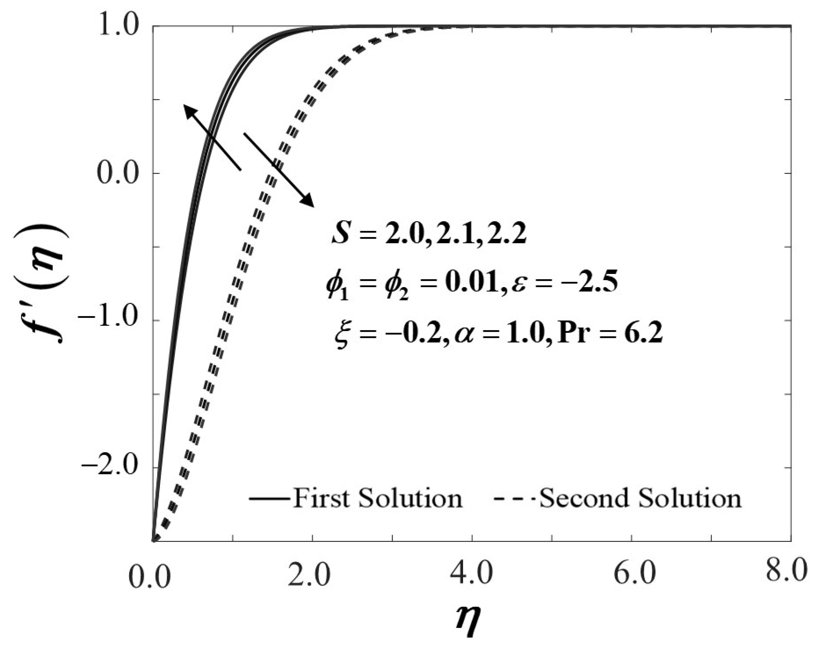
The suction parameter effect $S$ in accordance with the present study is revealed in Figure 4 and Figure 5. Figure 4 highlights the escalation of $S$ that amplifying $f^{″}\left(0\right)$ in the first solution of the hybrid nanofluid. Additionally, in this observation, the rising values of $S$ has expanded the dual solution domain $\epsilon ,$ causing an increment in the critical value $\left|{\epsilon }_c\right|$ on the moving plate of the hybrid nanofluid. This finding also contributes to the delay of the boundary layer separation process as $S$ improves (see Figure 6). Additionally, the skin friction coefficient recorded result is at the highest level with the largest value of $S$ in the hybrid nanofluid. Meanwhile, Figure 5 shows the value of $-{\theta }^{\prime }\left(0\right)$ increases with increasing value of $S$ on the moving plate surface in both solutions. It is found that the two solutions obtained are in line with the value addition. This occurrence is caused by the increment of suction values, allowing the flow of hybrid nanofluid to approach the flat plate surface, thus reducing the thickness of the boundary layer (see Figure 7). As a result, the hybrid nanofluid flow travels at a high velocity, enhancing the surface shear stress and thus intensifying the heat-transfer rate. In connection with the results discussed earlier in Figure 4 and Figure 5, Figure 6 scrutinises the suction parameter impact towards boundary layer velocity $f^{\prime }\left(\eta \right)$, while Figure 7 presents the distribution of temperature profile $\theta \left(\eta \right)$ by utilising hybrid nanofluid. As the number of suctions increases, the behaviour of the velocity profile is observed in an upward trend. This may be caused by the improvement of fluid viscosity in hybrid nanofluid with the increment of the suction effect. In contrast, small changes in the temperature profile distributions can be seen in Figure 7, where the temperature profile is reduced, especially when a dual system of nanoparticles is presented. This is due to an increase in the thermal conductivity of the mixing fluid, which improves heat-transfer performance and thus reduces temperature distributions. This scenario also occurred as a result of an increased amount of hot fluid being drawn away from the boundary layer, where the temperature decreased as the suction parameter value increased.

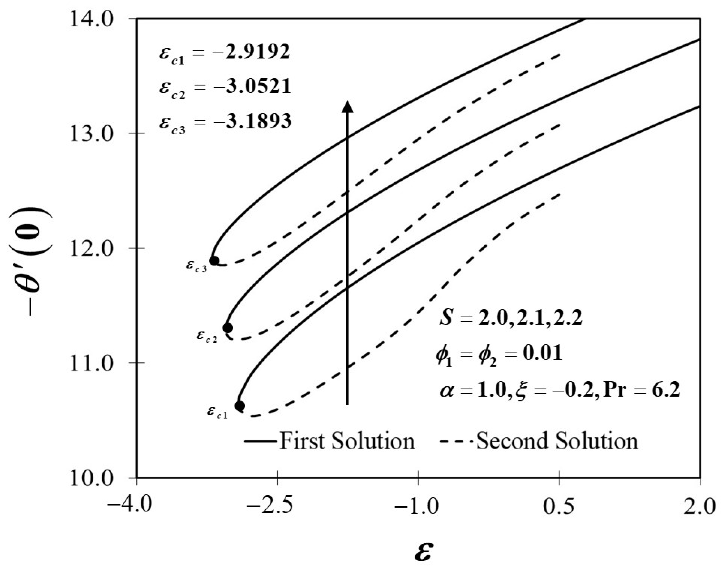
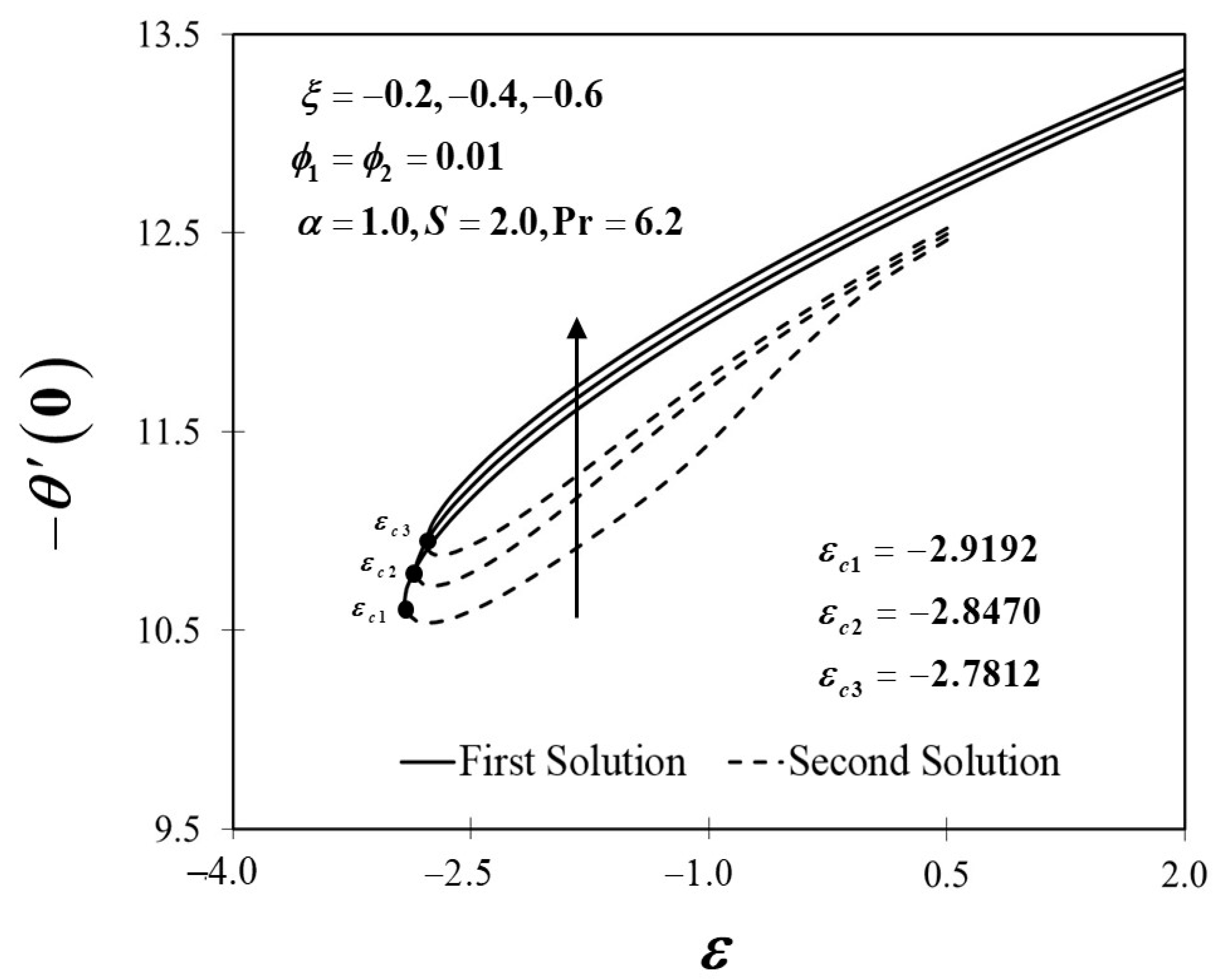
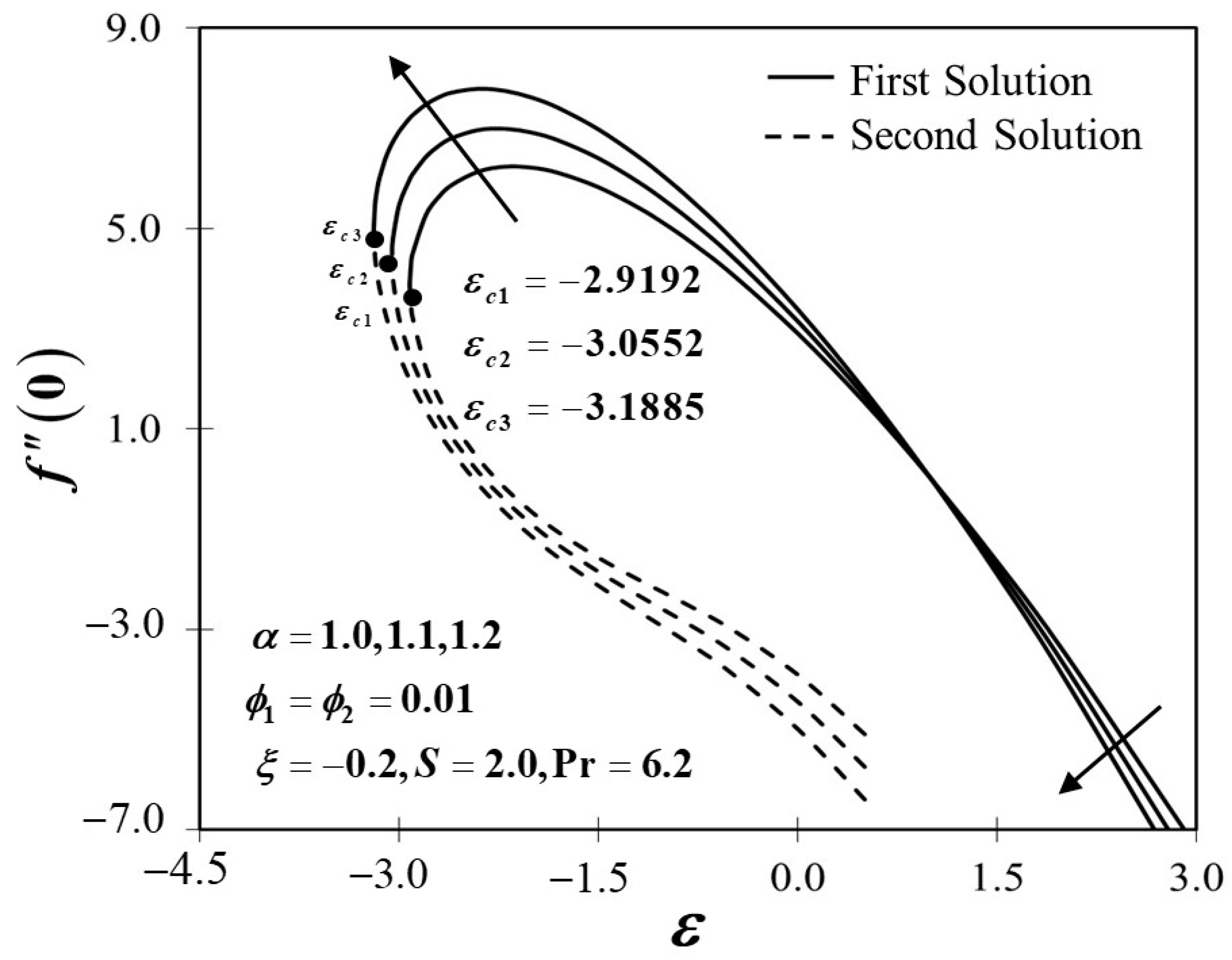
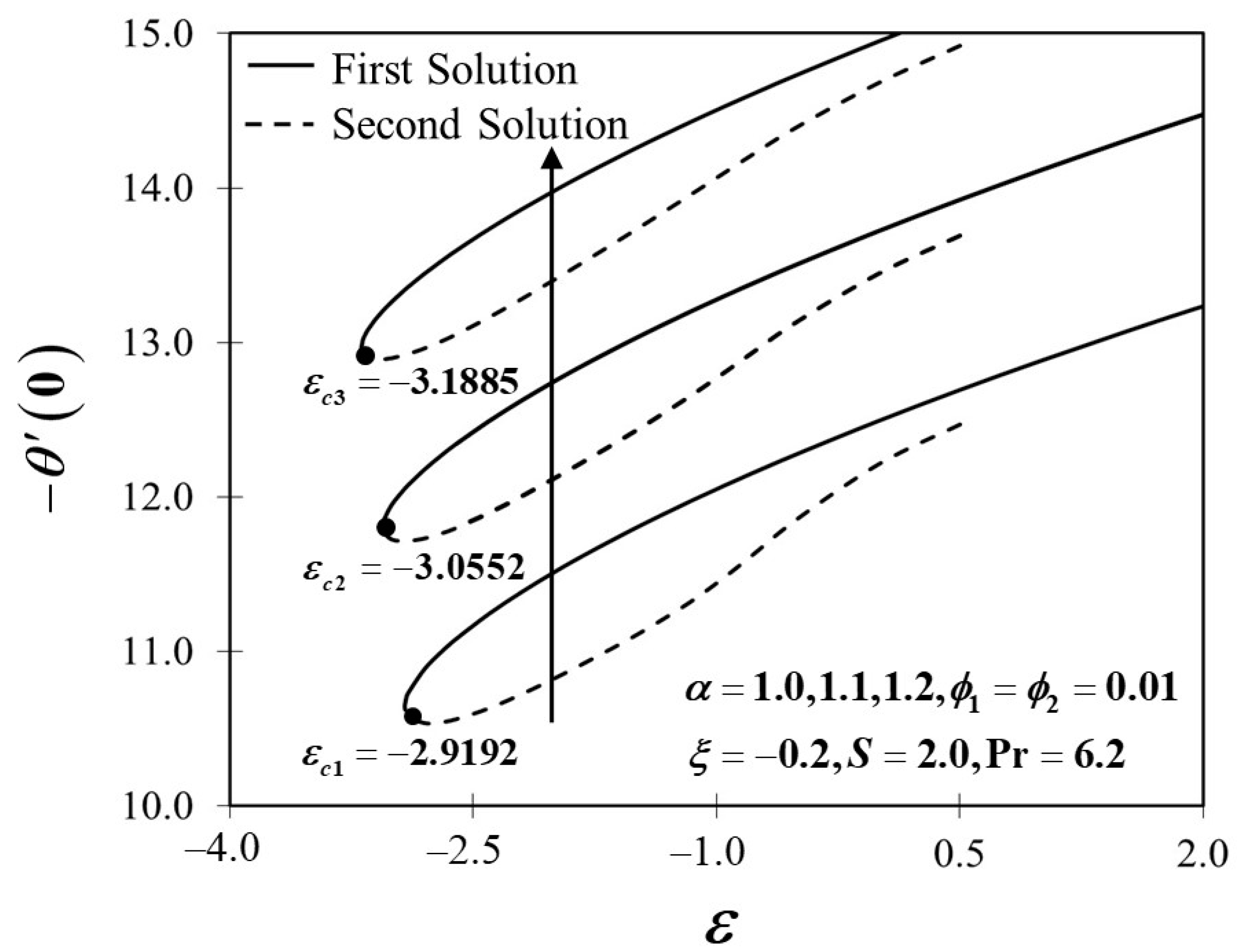
Additionally, this research is also concerned with adding the unsteadiness parameter $\xi$ into the hybrid nanofluid. Figure 8 portrays how decreasing $\xi$ decreases $f^{″}\left(0\right)$ in the first solution, while the reaction in the alternative solution was in the opposite direction. As $\xi$ declines, the thickness of the boundary layer broadens, limiting the gradient of velocity, with $f^{″}\left(0\right)$ therefore diminishing. Conversely, as $\xi$ reduces, the achieved results of $-{\theta }^{\prime }\left(0\right)$ expand in those solutions, as shown in Figure 9. The influence of the stagnation flow strength $\alpha$ in relation to $\epsilon$ towards moving plate is presented in Figure 10 and Figure 11. Figure 10 highlights that the escalation of $\alpha$ impulsively amplifies the trend of $f^{″}\left(0\right)$ in the first solution. This observation also indicates that a higher amount of $\alpha$ expands the flow, which causes the flow velocity to increase, resulting in a decrease in the thickness of the velocity boundary layer. In addition, Figure 10 also shows that when the sheet surface moves at a rate of $\epsilon =1.0$,$f^{″}\left(0\right)=0$. This explains the appearance of no frictional drag force on the progressed sheet surface, which is heated convectively. Sequentially, Figure 11 depicts the thermal efficiency, with $-{\theta }^{\prime }\left(0\right)$ intensifying in both solutions as the value of $\alpha$ increases in the hybrid nanofluid. The findings provide evidence that improving the strength of the stagnation flow encourages heat-transfer efficiency.

5. Conclusions

A numerical evaluation of the unsteady separated stagnation-point flow past a moving plate in a hybrid nanofluid was validated in this current work. The effects of various control parameters were investigated. Based on our findings, we can confirm dual solutions’ existence throughout the functioning fluids for a diverse variety of input variables. In comparison to a viscous fluid, nanofluid, and hybrid nanofluid, increasing the nanoparticle volume fraction concentration can significantly raise the skin friction coefficient while diminishing the heat-transfer rate. On the contrary, the inclusion of the suction parameter evidently improves the thermal performance efficiency. Due to the reduction values of the unsteadiness parameter, the skin friction coefficient declined but encouraged thermal productivity. A similar result is observed in the heat-transfer rate as the stagnation parameter strength improves in the hybrid nanofluid flow. The first solution’s reliability is secured by the stability analysis, whereas the second solution is confirmed as unstable.

References

- Blasius, H. Grenzschichten in Flu¨ssigkeiten mit kleiner Reibung. Z. Angew. Math. Phys. 1908, 56, 1–37. [Google Scholar]
- Prandtl, L. Über Flüssingkeitsbewegung bei sehr kleiner Reibung. In Proceedings of the Third International Mathematics Congress, Heidelberg, Germany, 8–13 August 1904; Volume 13, pp. 484–491. [Google Scholar]
- Sears, W.R.; Telionis, D.P. Unsteady boundary-layer separation. In Recent Research of Unsteady Boundary Layers, Proceedings of the International Union of Theoretical and Applied Mechanics, Tokyo, Japan, 13–17 September 1971; Eichelbrenner, E.A., Ed.; Laval University: Quebec, QC, Canada, 1972; pp. 404–447. [Google Scholar]
- Sears, W.R.; Telionis, D.P. Unsteady boundary-layer separation. Fluid dynamics of unsteady three- dimensional and separated flows. In Proceedings of the SQUID Workshop; Marshall, F.J., Ed.; Purdue University: West Lafayette, IN, USA, 1971; pp. 285–305. [Google Scholar]
- Lok, Y.Y.; Pop, I. Stretching or shrinking sheet problem for unsteady separated stagnation-point flow. Meccanica 2014, 49, 1479–1492. [Google Scholar] [CrossRef]
- Dholey, S.; Gupta, A.S. Unsteady separated stagnation-point flow of an incompressible viscous fluid on the surface of a moving porous plate. Phys. Fluids 2013, 25, 023601. [Google Scholar] [CrossRef]
- Dholey, S. On the fluid dynamics of unsteady separated stagnation-point flow of a power-law fluid on the surface of a moving flat plate. Eur. J. Mech. B Fluids 2018, 70, 102–114. [Google Scholar] [CrossRef]
- Renuka, A.; Muthtamilselvan, M.; Al-Mdallal, Q.M.; Doh, D.H.; Abdalla, B. Unsteady separated stagnation point flow of nanofluid past a moving flat surface in the presence of Buongiorno’s model. J. Appl. Comput. Mech. 2021, 7, 1283–1290. [Google Scholar]
- Fisher, E.G. Extrusion of Plastics; John Wiley & Sons, Inc.: New York, NY, USA, 1976. [Google Scholar]
- Rauwendaal, C. Polymer Extrusion; Hanser Publication: Munich, Germany, 1985. [Google Scholar]
- Hiemenz, K. Die Grenzschicht an einem in den gleichförmigen Flüssigkeitsstrom eingetauchten geraden Kreiszylinder. Dinglers Polytech. J. 1911, 326, 321–324. [Google Scholar]
- Homann, F. Der Einfluss grosser Zähigkeit bei der Strömung um den Zylinder und um die Kugel. Z. Angew. Math. Mech. 1936, 16, 153–164. [Google Scholar] [CrossRef]
- Wang, C.Y. Axisymmetric stagnation flow on a cylinder. Q. Appl. Math. 1974, 32, 207–213. [Google Scholar] [CrossRef] [Green Version]
- Takhar, H.S.; Chamkha, A.J.; Nath, G. Unsteady axisymmetric stagnation-point flow of a viscous fluid on a cylinder. Int. J. Eng. Sci. 1999, 37, 1943–1957. [Google Scholar] [CrossRef]
- Dholey, S. Magnetohydrodynamic unsteady separated stagnation-point flow of a viscous fluid over a moving plate. J. Appl. Math. Mech. 2016, 96, 707–720. [Google Scholar] [CrossRef]
- Jamaludin, A.; Nazar, R.; Pop, I. Mixed convection stagnation-point flow of Cross fluid over a shrinking sheet with suction and thermal radiation. Phys. A Stat. Mech. Appl. 2022, 585, 126398. [Google Scholar] [CrossRef]
- Choi, S.U.S. Enhancing thermal conductivity of fluids with nanoparticles. In Proceedings of the 1995 International Mechanical Engineering Congress and Exhibition, San Francisco, CA, USA, 12–17 November 1995; Volume 66, pp. 99–105. [Google Scholar]
- Suresh, S.; Venkitaraj, K.P.; Selvakumar, P. Synthesis, characterisation of Al2O3-Cu nano composite powder and water based nanofluids. Adv. Mater. Res. 2011, 328–330, 1560–1567. [Google Scholar] [CrossRef]
- Chamsa-ard, W.; Brundavanam, S.; Fung, C.C.; Fawcett, D.; Poinern, G. Nanofluid types, their synthesis, properties and incorporation in direct solar thermal collectors: A review. Nanomaterials 2017, 7, 131. [Google Scholar] [CrossRef]
- Sharma, R.; Ishak, A.; Pop, I. Dual solution of unsteady separated stagnation-point flow in a nanofluid with suction: A finite element analysis. Indian J. Pure Appl. Phys. 2017, 55, 275–283. [Google Scholar]
- Roşca, N.C.; Roşca, A.V.; Pop, I. Unsteady separated stagnation-point flow and heat transfer past a stretching/shrinking sheet in a copper-water nanofluid. Int. J. Numer. Methods Heat Fluid Flow 2019, 29, 2588–2605. [Google Scholar] [CrossRef]
- Oztop, H.F.; Abu-Nada, E. Numerical study of natural convection in partially heated rectangular enclosures filled with nanofluids. Int. J. Heat Fluid Flow 2008, 29, 1326–1336. [Google Scholar] [CrossRef]
- Das, S.K.; Choi, S.U.S.; Yu, W.; Pradeep, Y. Nanofluids: Science and Technology; John Wiley & Sons, Inc.: Hoboken, NJ, USA, 2008. [Google Scholar]
- Minkowycz, W.J.; Sparrow, E.; Abraham, J.P. Nanoparticle Heat Transfer, and Fluid Flow; CRC Press: Boca Raton, FL, USA, 2012. [Google Scholar]
- Shenoy, A.; Sheremet, M.; Pop, I. Convective Flow and Heat Transfer from Wavy Surfaces: Viscous Fluids, Porous Media and Nanofluids; CRC Press: Boca Raton, FL, USA, 2016. [Google Scholar]
- Nield, D.A.; Bejan, A. Convection in Porous Media; Springer: New York, NY, USA, 2017. [Google Scholar]
- Merkin, J.H.; Pop, I.; Lok, Y.Y.; Groşan, T. Similarity Solutions for the Boundary Layer Flow and Heat Transfer of Viscous Fluids, Nanofluids, Porous Media and Micropolar Fluids; Elsevier: Oxford, UK, 2021. [Google Scholar]
- Buongiorno, J.; Venerus, D.C.; Prabhat, N.; McKrell, T.; Townsend, J.; Christianson, R.; Tolmachev, Y.V.; Keblinski, P.; Hu, L.W.; Alvaro, J.L.; et al. A benchmark study on the thermal conductivity of nanofluids. J. Appl. Phys. 2009, 106, 1–14. [Google Scholar] [CrossRef] [Green Version]
- Manca, O.; Jaluria, Y.; Poulikakos, D. Heat transfer in nanofluids. Adv. Mech. Eng. 2010, 2, 38082. [Google Scholar] [CrossRef]
- Mahian, O.; Kianifar, A.; Kalogirou, S.A.; Pop, I.; Wongwises, S. A review of the applications of nanofluids in solar energy. Int. J. Heat Mass Transfer 2013, 57, 582–594. [Google Scholar] [CrossRef]
- Mahian, O.; Kolsi, L.; Amani, M.; Estellé, P.; Ahmadi, G.; Kleinstreuer, C.; Marshall, J.S.; Siavashi, M.; Taylor, R.A.; Niazmand, H. Recent advances in modeling and simulation of nanofluid flows—Part I: Fundamentals and theory. Phys. Rep. 2019, 790, 1–48. [Google Scholar] [CrossRef]
- Kasaeian, A.; Daneshazarian, R.; Mahian, O.; Kolsi, L.; Chamkha, A.J.; Wongwises, S.; Pop, I. Nanofluid flow and heat transfer in porous media: A review of the latest developments. Int. J. Heat Mass Transf. 2017, 107, 778–791. [Google Scholar] [CrossRef]
- Gupta, H.; Agrawal, G.; Mathur, J. An overview of nanofluids: A new media towards green environment. Int. J. Environ. Sci. 2012, 3, 433–440. [Google Scholar]
- Ebrahimi, A.; Tamnanloo, J.; Mousavi, S.H.; Soroodan Miandoab, E.; Hosseini, E.; Ghasemi, H.; Mozaffari, S. Discrete-continuous genetic algorithm for designing a mixed refrigerant cryogenic process. Ind. Eng. Chem. Res. 2021, 60, 7700–7713. [Google Scholar] [CrossRef]
- Darjani, S.; Koplik, J.; Pauchard, V.; Banerjee, S. Glassy dynamics and equilibrium state on the honeycomb lattice: Role of surface diffusion and desorption on surface crowding. Phys. Rev. E 2021, 103, 022801. [Google Scholar] [CrossRef]
- Senyuk, B.; Mozaffari, A.; Crust, K.; Zhang, R.; de Pablo, J.J.; Smalyukh, I.I. Transformation between elastic dipoles, quadrupoles, octupoles, and hexadecapoles driven by surfactant self-assembly in nematic emulsion. Sci. Adv. 2021, 7, eabg0377. [Google Scholar] [CrossRef] [PubMed]
- Mozaffari, S.; Ghasemi, H.; Tchoukov, P.; Czarnecki, J.; Nazemifard, N. Lab-on-a-chip systems in asphaltene characterization: A review of recent advances. Energy Fuels 2021, 35, 9080–9101. [Google Scholar] [CrossRef]
- Xian, H.W.; Sidik, N.A.C.; Aid, S.R.; Ken, T.L.; Asako, Y. Review on preparation techniques, properties and performance of hybrid nanofluid in recent engineering applications. J. Adv. Res. Fluid Mech. Therm. Sci. 2018, 45, 1–13. [Google Scholar]
- Devi, S.S.; Devi, S.P. Numerical investigation of three-dimensional hybrid Cu–Al2O3/water nanofluid flow over a stretching sheet with effecting Lorentz force subject to Newtonian heating. Can. J. Phys. 2016, 94, 490–496. [Google Scholar] [CrossRef]
- Devi, S.P.A.; Devi, S.S.U. Numerical investigation of hydromagnetic hybrid Cu–Al2O3/water nanofluid flow over a permeable stretching sheet with suction. Int. J. Nonlinear Sci. Numer. Simul. 2016, 17, 249–257. [Google Scholar] [CrossRef]
- Devi, S.U.; Devi, S.P.A. Heat transfer enhancement of Cu−Al2O3/water hybrid nanofluid flow over a stretching sheet. J. Niger. Math. Soc. 2017, 36, 419–433. [Google Scholar]
- Takabi, B.; Salehi, S. Augmentation of the heat transfer performance of a sinusoidal corrugated enclosure by employing hybrid nanofluid. Adv. Mech. Eng. 2014, 6, 147059. [Google Scholar] [CrossRef]
- Ghalambaz, M.; Ros, N.C.; Ros, A.V.; Pop, I. Mixed convection and stability analysis of stagnation-point boundary layer flow and heat transfer of hybrid nanofluids over a vertical plate. Int. J. Numer. Methods Heat Fluid Flow 2020, 30, 3737–3754. [Google Scholar] [CrossRef]
- Waini, I.; Ishak, A.; Pop, I. Hybrid nanofluid flow towards a stagnation point on a stretching/shrinking cylinder. Sci. Rep. 2020, 10, 9296. [Google Scholar] [CrossRef]
- Khashiʼie, N.S.; Arifin, N.M.; Pop, I.; Wahid, N.S. Effect of suction on the stagnation point flow of hybrid nanofluid toward a permeable and vertical Riga plate. Heat Transf. 2021, 50, 1895–1910. [Google Scholar] [CrossRef]
- Zainal, N.A.; Nazar, R.; Naganthran, K.; Pop, I. Stability analysis of unsteady MHD rear stagnation point flow of hybrid nanofluid. Mathematics 2021, 9, 2428. [Google Scholar] [CrossRef]
- Zainal, N.A.; Nazar, R.; Naganthran, K.; Pop, I. Impact of anisotropic slip on the stagnation-point flow past a stretching/shrinking surface of the Al2O3-Cu/H2O hybrid nanofluid. Appl. Math. Mech. 2020, 41, 1401–1416. [Google Scholar] [CrossRef]
- Zainal, N.A.; Nazar, R.; Naganthran, K.; Pop, I. Unsteady MHD stagnation point flow induced stretching/shrinking sheet of hybrid nanofluid by exponentially permeable. Eng. Sci. Technol. Int. J. 2021, 24, 1201–1210. [Google Scholar] [CrossRef]
- Ranga Babu, J.A.; Kumar, K.K.; Rao, S.S. State-of-art review on hybrid nanofluids. Renew. Sustain. Energy Rev. 2017, 77, 551–565. [Google Scholar] [CrossRef]
- Huminic, G.; Huminic, A. Hybrid nanofluids for heat transfer applications—A state-of-the art review. Int. J. Heat Mass Transf. 2018, 125, 82–103. [Google Scholar] [CrossRef]
- Dholey, S. Unsteady separated stagnation-point flow over a permeable surface. Z. Angew. Math. Phys. 2019, 70, 1–19. [Google Scholar] [CrossRef]
- Merkin, J.H. Mixed convection boundary layer flow on a vertical surface in a saturated porous medium. J. Eng. Math. 1980, 14, 301–313. [Google Scholar] [CrossRef]
- Merkin, J.H. On dual solutions occurring in mixed convection in a porous medium. J. Eng. Math. 1986, 20, 171–179. [Google Scholar] [CrossRef]
- Weidman, P.D.; Kubitschek, D.G.; Davis, A.M.J. The effect of transpiration on self-similar boundary layer flow over moving surfaces. Int. J. Eng. Sci. 2006, 44, 730–737. [Google Scholar] [CrossRef]
- Harris, S.D.; Ingham, D.B.; Pop, I. Mixed convection boundary-layer flow near the stagnation point on a vertical surface in a porous medium: Brinkman model with slip. Transp. Porous Media 2009, 77, 267–285. [Google Scholar] [CrossRef]
- Shampine, L.F.; Reichelt, M.W.; Kierzenka, J. Solving boundary value problems for ordinary differential equations in Matlab with bvp4c. Tutor. Notes 2000, 2000, 1–27. [Google Scholar]
- Wang, C.Y. Stagnation flow towards a shrinking sheet. Int. J. Non. Linear. Mech. 2008, 43, 377–382. [Google Scholar] [CrossRef]
- Ishak, A.; Lok, Y.Y.; Pop, I. Stagnation-point flow over a shrinking sheet in a micropolar fluid. Chem. Eng. Commun. 2010, 197, 1417–1427. [Google Scholar] [CrossRef]
- Sarkar, J.; Ghosh, P.; Adil, A. A review on hybrid nanofluids: Recent research, development and applications. Renew. Sustain. Energy Rev. 2015, 43, 164–177. [Google Scholar] [CrossRef]
- Khashi’ie, N.S.; Arifin, N.M.; Pop, I.; Wahid, N.S. Flow and heat transfer of hybrid nanofluid over a permeable shrinking cylinder with Joule heating: A comparative analysis. Alex. Eng. J. 2020, 59, 1787–1798. [Google Scholar] [CrossRef]
- Khashi’ie, N.S.; Arifin, N.M.; Nazar, R.; Hafidzuddin, E.H.; Wahi, N.; Pop, I. Magnetohydrodynamics (MHD) axisymmetric flow and heat transfer of a hybrid nanofluid past a radially permeable stretching/shrinking sheet with Joule heating. Chin. J. Phys. 2020, 64, 251–263. [Google Scholar] [CrossRef]
Figure 1.
The geometrical coordinates and flow pattern.
Figure 2.
Trend of towards by assorted .
Figure 3.
Figure 4.
Figure 5.
Figure 6.
Velocity profile towards by assorted .
Figure 7.
Temperature distribution towards by assorted .
Figure 8.
Figure 9.
Figure 10.
Figure 11.